SICE Annual Conference 2013 September 14-17, 2013, Nagoya University, Nagoya, Japan
Integrating On-board Diagnostics Speed Data with Sparse GPS Measurements for Vehicle Trajectory Estimation Sumeet Kumar⇤1 , Johannes Paefgen⇤2 , Erik Wilhelm3 and Sanjay E. Sarma1 Equal contribution Department of Mechanical Engineering, Massachusetts Institute of Technology, Cambridge, MA, 02139 USA (E-mail:
[email protected],
[email protected]) 2 Department of Management, Technology, and Economics, ETH Zurich, Weinbergstrasse 56/58, 8092 Zurich, Switzerland (E-mail:
[email protected]) 3 The Engineering Product Development Pillar at the Singapore University of Technology and Design, Singapore 138682 (E-mail:
[email protected]) ⇤
1
Abstract: We evaluate the integration of on-board diagnostics (OBD) speed measurements with sparse and/or missing GPS data for vehicle trajectory estimation using an extended Kalman filter. The suggested framework is relevant to the deployment of low-power, low-cost GPS receivers in the context of mobile and pervasive sensing. Our algorithm is capable of handling sensors at different sampling rates and comprises an accelerometer error model that significantly improves trajectory estimation. Based on field data, we evaluate its performance by simulating deliberately reduced GPS sampling rates, random GPS outages, and varying base sampling rates of the Kalman filter estimation loop. We achieve robust performance in estimating the driven distance and a vehicle trajectory with GPS data downsampled from 10 Hz to 0.02 Hz. We also demonstrate that for random GPS omissions of up to two thirds of the samples, the root mean squared error of position estimates is less than 4 m with GPS data downsampled by a factor of 10. Keywords: On-Board Diagnostics, GPS, Vehicle Navigation, Extended Kalman Filter
1. INTRODUCTION
proach involves using a vehicle motion model in combination with a Kalman filter to estimate states in the presence of noisy GPS and IMU data. Zhang et al. [10] compared the extended Kalman filter with the unscented Kalman filter for GPS/IMU integration. Carom et al. [11] included contextual information to define validity domains of sensor data and reject bad sensor measurements. Adaptive Kalman filtering [12] and factor graph based smoothing [13] have also been studied for trajectory estimation. On-board-diagnostics (OBD) monitors engine health and vehicle components and allows services to be performed based on real-time and recorded events. Since 1996, all cars sold in US were made mandatory to have OBD specifications [14]. An important vehicle motion parameter that can be obtained through OBD is speedometer data. Contrary to other vehicle network variables such as odometer readings, OBD data is accessible in a manufacturer-independent, standardized format. Further, OBD scan tools have shown significant improvement in recent years and now have the capability of real time data logging through a serial port or wireless protocols like bluetooth and wifi [15]. These tools have the potential for integrating speedometer data with existing GPS hardware and even mobile phones. In this paper, our objectives are to robustly estimate driven distance and reconstruct a vehicle trajectory in the presence of (i) deliberate GPS downsampling and (ii) random GPS outage. To achieve this, we extend the GPS/IMU sensor fusion to include dead reckoning through the OBD speed data. Our sensor system comprises a low cost GPS, IMU and OBD scan tool.
Vehicle based sensing has attracted significant attention in the past decade. The availability of cost-effective sensors and their compact form factor make it practical for them to be mounted on vehicles and implement large scale urban pervasive sensing [1]. Further, the emergence of smartphones, embedded with Global Positioning System (GPS) receivers, have broadened the extent of vehicle based sensing [2]. Several key applications are emerging that require vehicle location information, like traffic monitoring and management services [3], route planning [4], [5], geographical social network [6] and vehicle based urban sensing [2], [7]. Successful implementation of such services requires accurate vehicle location and trajectory information. GPS, providing absolute geographic location, is typically used to obtain location information of the driving vehicles and has an an accuracy of few meters [8]. Differential GPS can have an improved sub-meter accuracy [9]. GPS, in general, suffers from low reliability especially in urban driving conditions due to multipath effects and poor satellite signal [10]. Further, we would prefer to operate GPS receivers at lower sampling rates which favors lower bandwidth and power consumption but limits the spatial resolution of location information. Hence there is a need for developing robust methods for using low frequency, noisy GPS data to accurately estimate vehicle trajectories. Researchers have made significant progress in developing sensor fusion algorithms for combining GPS data with inertial measurement units (IMU). A typical ap2302
PR0001/13/0000-2302 ¥400 © 2013
SICE Annual Conference 2013 September 14-17, 2013, Nagoya, Japan
x
b
The paper differs from prior research in two significant aspects: Firstly, our approach does not depend on map data for the estimation of driving parameters, which makes it suitable for light-weight applications that run on mobile phones or retrofitted telematics devices in vehicles. Secondly, by using only an off-the-shelf IMU in combination with OBD data accessed via the standardized connector, our system is straightforward to replicate independent of vehicle make or model. While studies that leverage map data and more sophisticated sensing solutions [16] are likely to achieve better estimation performance than the suggested approach, they are aimed at professional applications and more difficult to implement. We develop an online extended hybrid Kalman filter that includes a model of accelerometer noise and handles different sensors at different sampling rates. We study the error in the vehicle trajectory estimation and the driven distance with downsampling of GPS data, and under simulation of random outage as a Bernoulli process. We show that our approach yields robust estimates for sampling rates reduced by a factor of up to 500. We also demonstrate that random GPS outage can be handled well within our framework. The remainder of this paper is organized as follows. Section 2 develops our framework for vehicle trajectory estimation. We discuss the vehicle and the measurement model, derive an appropriate discrete-time state space model, and present an extended Kalman filter formulation. In Section 3, we carry out evaluation of the proposed framework based on driving data. We devise an evaluation methodology, define two performance metrics and present simulation results. In Section 4 we conclude our work and provide a discussion.
(X,Y) θ
Fig. 1 Simplified vehicle motion model in Cartesian coordinates Let the acceleration measured in B be (axb , ayb ). Combining Eqn. 1 and Eqn. 2, we obtain the following equations: v˙ = axb , ✓˙ = ay /v.
As discussed before, we use three sensors in our study: GPS, IMU and OBD scan tool. Accelerometers on the IMU provide vehicle accelerations in the frame B. Typically, the low cost accelerometers which we use in our study, suffer from a significant scaling and bias error that can be modeled as: axb = su1 + b1 , ayb = su2 + b2 ,
(4)
where u1 and u2 are the accelerometer measurements along the axis xb and yb respectively, s is the accelerometer scaling factor and b1 and b2 are the accelerometer biases. We assume that the scaling factor s is the result of external parameters such as temperature fluctuations and may thus be assumed identical for both, lateral and longitudinal accelerations. Under this assumption, we can use OBD speed data to not only correct for accelerometer scaling in the direction xb , but also in yb . Furthermore, periods of vehicle stoppage as evident from OBD data allow for direct inference of accelerometer biases. GPS provides noisy latitude ( ) and longitude ( ) estimate of the vehicle. Assuming earth to be spherical, we can convert ( , ) to cartesian coordinate using the following equations: X = R cos( Y = R(
m )(
m ),
(5)
m ),
PN
where R is Earth’s radius, and m = i=1 i /N and PN = /N are latitude and longitude averaged m i=1 i over a set of N measurements. OBD scan tool measures vehicle speed along xb and is denoted by v.
X˙ = v cos ✓, Y˙ = v sin ✓, (1)
2.1 Discrete-Time State Space Model We represent the system by a state vector x(t) = (X, Y, d, v, ✓, b1 , b2 , s), where d is an auxiliary state variable representing aggregated driven distance. Assuming
Further, we have the following no slip condition: X˙ sin ✓ = 0.
(3)
b
We first develop equations of motions that form the basis of Kalman filter based sensor fusion. We model the car as a unicycle, a viable assumption when considering only linear vehicle dynamics [17] with the constraint that the vehicle moves along the trajectory with no slip. As shown in Fig. 1, G is the frame fixed to the ground with respect to which we aim to estimate the position of the car (X, Y ). B is the body frame attached to the vehicle and ✓ (heading) is the angle that xb makes with the x axis. Typically two drive controls are assumed, velocity, v, leading to forward motion and an angular velocity (rotation of the frame B), !, for turns. This yields the following equations of motion:
Y˙ cos ✓
G
x
2. VEHICLE TRAJECTORY ESTIMATION
✓˙ = !.
yb
B y
(2) 2303
SICE Annual Conference 2013 September 14-17, 2013, Nagoya, Japan
bias and scaling errors as constant, yields the following continuous, non-linear state space model: 2 3 x4 cos x5 6 x4 sin x5 7 6 7 6 7 x 4 7 x˙ = 6 (6) 6 x8 u1 + x6 7 . 6 7 4(x8 u2 + x7 )/x4 5 03⇥1
trix: F(k) = 2
6 6 6 6 =6 6 6 6 4
Note that we include IMU readings as system input, as they represent our best knowledge of the driver’s action assuming that throttle and steering wheel input are inaccessible. Furthermore, using them as a measurement input would require an extension of Eqn. 6 to include second-derivative terms. Applying Euler’s Forward Method with step size T to Eqn. 6, we obtain the discrete state update as: x(k + 1) = f (x(k), u(k)) 2 3 x4 (k) cos x5 (k) 6 x4 (k) sin x5 (k) 7 6 7 6 7 x4 (k) 6 = x(k) + T 6x (k)u (k) + x (k)7 7. 8 1 6 6 x8 (k)u2 (k)+x7 (k) 7 4 5
= ˆ (k|k),u(k) x
05⇥3
cos x5 sin x5 1 0 x8 u2 +x7 x24
x4 sin x5 x4 cos x5 0 0 0 03⇥8
0 0 0 1 0
0 0 0 0 1 x4
3 0 07 7 07 7 u1 7 , u2 7 7 x4 7 5
(9)
evaluated at the current state estimate and IMU input vector u. In parametrizing the process noise covariance matrix Q, we chose comparatively high values for entries corresponding to steps involving updates of u1 and u2 , while the bias and scaling error terms received low values as they vary only slowly over time. We assume independence among process noise and Q to be a diagonal matrix. For the measurement update, a vector
(7)
z(k) = h(ˆ x(k|k
x4 (k)
1)) = Hˆ x(k|k
1)
(10)
is defined that maps the system states to sensor observations. As stated in the Introduction, our objective is to estimate the true vehicle trajectory with noisy and temporarily unavailable GPS measurements. Therefore, we use two different measurement vectors depending on the availability of GPS data: 2 3 X ⇥ ⇤ ˜(k) = vx , z(k) = 4 Y 5 , z with vx ⇥ ⇤T H= 1 1 0 1 0 0 0 0 and ⇥ ⇤T ˜ = 0 0 0 1 0 0 0 0 respectively. (11) H
03⇥1
As the computation of changes in heading (✓) becomes numerically unstable for velocities close to zero, we replace the corresponding state update equation with x5 (k + 1) = x5 (k) if x4 (k) < vmin = 2 m/s, i.e. assuming constant heading. Accelerometer readings u1 and u2 are affected by vehicle yaw and roll, i.e. rotations about the xb and yb axes. Such rotations are caused either by road inclination, or by load changes during cornering and vehicle acceleration. While in theory these dynamics could be explicitly modeled, we do not consider vehicle yaw and roll in our analysis. Doing so would require more sensing inputs and higher quality of measurements due to the increased number of states in the system. However, the simplified bias and scaling error model laid out above can account for changes in vehicle pose to some extent. When driving uphill, for instance, a constant gravity vector component of u1 will be compensated for due to the discrepancy between u1 and OBD readings.
In the absence of GPS measurements, our EKF imple˜ which renders the states x5 (vementation switches to H hicle heading) and x7 (lateral-direction IMU bias) unreachable. The measurement noise covariance matrix R, is parametrized according to specifications of the used sensors with the assumption of independence among measurement errors. If both GPS and OBD measurements are available, it is set to R = diag(32 , 32 , 0.4472 ), corresponding to a standard deviation of 3 m around the true position for GPS. We have the following set of update equations:
2.2 Extended Kalman Filter with Hybrid Measurement Update Due to the non-linear system dynamics, we implement a variant of the well-known discrete-time Extended Kalman filter (EKF) [10]. For both, state update and measurement update, we assume zero-mean, additive noise that follows a multivariate Gaussion distribution. The EKF state estimate update then is ˆ (k + 1|k) = f (ˆ x x(k|k), u(k)).
@f @x
ˆ (k + 1|k) = f (ˆ x x(k|k), u(k)) P(k + 1|k) = F(k)P(k|k)F(k)T + Q ˆ (k + 1) = z(k + 1) h(ˆ y x(k + 1|k)) S(k + 1) = HP(k + 1|k)HT + R K(k + 1) = P(k + 1|k)HT S(k + 1) 1 ˆ (k + 1|k + 1) = x ˆ (k + 1|k) + K(k + 1)ˆ x y(k + 1) P(k + 1|k + 1) = (I K(k + 1)H)P(k + 1|k). (12)
(8)
The error covariance matrix P(k|k) for state estimates ˆ (k|k) is updated using the linearized state transition max 2304
SICE Annual Conference 2013 September 14-17, 2013, Nagoya, Japan
˜ in the ˜ and H with H Note that we change z with z absence of GPS measurements. We remark that this hybrid formulation is straightforward to adapt to further available measurements such as odometer, gyroscope, and magnetic field sensors by modifications analogous to Eqn. 11.
In order to obtain the true states x1 , x2 , x3 for error calculation, we compute a reference trajectory from the 10 Hz full resolution GPS data using our algorithm. These errors capture two important aspects of vehicle navigation solutions. The driven distance estimate is relevant to applications that are concerned with the extent of vehicle usage. The position-RMSE is relevant where a reconstruction of the precise vehicle trajectory is used, e.g., as a reference for environmental sensing tasks. It is also a prerequisite to map matching techniques that fit the estimated positions into digital maps [18]. As an estimate for traveled distance without the use of OBD data, we aggregate the distance increments between consecutive points of the downsampled GPS measurement vectors. For this distance estimate, we compute ✏d and compare it to the EKF generated error metric. We do not compute ✏r for this scenario, as there is no obvious interpolation scheme between downsampled GPS measurements in the absence of speed information. The assumption of constant speed required for a simple linear interpolation to estimate locations in intermediate times does not appear justified.
3. EMPIRICAL VALIDATION 3.1 Procedure We use a Ford Focus hatchback for collecting data. Our sensor system includes a low cost GPS (Qstarz BTQ818XT), IMU (9 degree of freedom Razor IMU) and OBDLink SX scan tool [15]. We collect data from a closed-loop route in Cambridge, MA with the total driving distance to be around 3.35 km. All the sensors are integrated with a laptop to log data during driving. The GPS uses a bluetooth protocol to send data to the laptop. The IMU is connected to an Arduino Mega and attached to a roof rack placed on top of the car. The IMU is mounted with its x-axis aligned along xb and its y-axis along yb . Through a USB cable, the Arduino and the OBD scan tool are connected to the laptop. We developed our own code to log data from the three sensors at 10 Hz. To assess the impact of an intentionally reduced GPS sampling rate, we systematically downsample the original GPS data collected at 10 Hz. The measurements vector hence includes unobserved GPS data and is addressed through the hybrid scheme discussed in Section 2.2. For each GPS sampling time, we execute an on-line EKF estimation implementing state updates at 10 Hz and store the resulting state trajectory. We extend the analysis of deliberate GPS downsampling by an emulation of GPS unavailability. For every entry in the downsampled GPS-measurement vector, we determine its inclusion in the EKF estimation as the outcome of a Bernoulli trial with a certain probability of not observing GPS data (denoted by p). We choose p = {1/3, 1/2, 2/3} and for each p run 50 simulations in order to obtain mean and standard deviation of the performance metrics to be discussed in the next subsection. We carry out all computations in Mathworks Matlab R2012a.
Error state estimate
0.1
|ˆ x3 (K) x3 (K)| , x3 (K)
k=1
−0.05
(x8 − 1) 100
200
300 Time (s)
400
500
400
500
600
(a) OBD−II measurement
50 Velocity (m/s)
40
t 0
(u1) dt
t 0
(x8 u1 + x6) dt
30 20 10 0
0
100
200
300 Time (s)
600
(b)
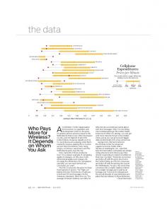
Fig. 2 (a) Scaling and bias estimates as a function of time; (b) OBD data, raw accelerometer integral and scaling, bias corrected accelerometer integral.
(13)
x1 (k))2 + (ˆ x2 (k)
x7
0
3.3 Results First, we evaluate the evolution of scaling and bias estimates at 10Hz GPS sampling frequency as depicted in Fig.2a. These states improve the accelerometer measurements to be included as an input in the EKF algorithm. Fig.2b shows the integrated acceleration u1 before and after application of the error model together with the observed OBD speed.
where index K denotes the final state. Secondly, we compute the root mean square error of position estimates v u K h u1 X ✏r = t (ˆ x1 (k) K
x6
0
−0.1
3.2 Performance Metrics We define two performance criteria for the proposed estimation technique. First, we compute the relative error in the driven distance estimate ✏d =
0.05
i 2 x2 (k)) . (14)
2305
SICE Annual Conference 2013 September 14-17, 2013, Nagoya, Japan
estimate that is largely unaffected by these sources of errors.
800 600
10
200 0 −200 −400 −600 −600
−400
−200
0 x (m)
200
400
6 4 2
600
0 −1 10
(a)
0
1
800
10 10 GPS Sampling Time Ts (s)
600
Fig. 4 Variation of ✏d with Ts
400 y (m)
Aggregated GPS 10Hz EKF estimate
8 εd (%)
y (m)
400
200 0 −200 −400 −600 −600
−400
−200
0 x (m)
200
400
600
(b)
Fig. 3 Comparison of vehicle reference trajectory (in black) with EKF trajectory estimate (in red) for different GPS sampling time: (a) Ts = 5 s; (b) Ts = 20 s.
2
10
Next, we evaluate the performance of the proposed algorithm under random omissions of GPS measurements. Fig.5a shows that ✏r is acceptable up to Ts = 1 s, after which we observe a sharp increase in the RMSE of the vehicle position estimates. As expected, the error is higher for higher probabilities of GPS outage. Fig.5b shows a similar trend, though the driven distance error is acceptable even for higher values of Ts . For driving scenarios where the GPS availability may vary across the route, this suggests an adaptive sampling strategy. Adjusting the GPS sampling rate in accordance with observed GPS outages will lead to higher accuracy in trajectory estimation. 25 20 εr (m)
For the generation of sparse GPS measurement vectors, we select an exponentially increasing series of integers from 1 to 500 as downsampling factors. For each factor, a new sample interval time Ts is obtained for GPS measurements. We then use our hybrid EKF framework to estimate trajectories and evaluate performance metrics ˜ where at 10Hz, switching between the measurement z GPS points are not available, and z otherwise. Fig.3a and 3b depict two examples of vehicle trajectory reconstructions at Ts = 5 s and 20 s, respectively, together with a Ts = 0.1 s reference trajectory. At a downsampling factor of 50 (Ts = 5 s) we achieve robust replication of the reference trajectory. At a downsampling factor of 200 (Ts = 20 s), a segment-wise distortion of the estimated trajectory is observed. These segments mostly exhibit errors in the vehicle heading estimate, while segment lengths show minor deviations. In Fig.4 we report the variation of ✏d as a function of Ts . For EKF-based trajectory reconstructions, ✏d is lower than 0.1% for Ts < 1 s and lower than 1% for Ts < 50 s. The aggregated distance increments (cf. Section 3.2) exhibit a higher driven distance error. The U-shaped distribution of the errors can be attributed to GPS noise aggregation at lower Ts and the failure to capture sufficient path curvature details at higher Ts . On the other hand, our hybrid EKF method provides a robust driven distance
15
p = 1/3 p = 1/2 p = 2/3 p=0
10 5 0 −1 10
0
10 Ts (s)
1
10
(a) 1
εd (%)
0.8 0.6
p = 1/3 p = 1/2 p = 2/3 p=0
0.4 0.2 0 −1 10
0
10 Ts (s)
1
10
(b)
Fig. 5 Comparison of the performance metrics for different GPS outage probability: (a) ✏r and (b) ✏d . The solid lines indicate the mean of the metric while the dashed lines indicate mean +/- 12 standard deviation. We further reduce the base sampling rate of the 2306
SICE Annual Conference 2013 September 14-17, 2013, Nagoya, Japan
KF Sampling Time Ts,KF [s]
εr (m)
handle sparse and/or missing GPS data. We evaluated an extended Kalman filter for the reconstruction of a vehicle trajectory and the driven distance in the presence of sparse GPS data. By including bias and scaling error of the IMU measurements in the state space model, the performance of the estimator was considerably improved. As expected, the inclusion of OBD data enabled consistent estimates of the driven distance even at GPS sampling rates below 0.02 Hz. A comparison with the aggregated GPS distance increments demonstrated that the estimated distance suffered neither from the integration of errors at high sampling frequencies, nor from the exclusion of path details at low sampling frequencies. The estimator was also able to maintain low deviations from a reference trajectory in terms of root mean squared position errors. We showed that for random GPS sample omissions of up to two thirds of the samples, the error remained below 4 m for GPS sampling rate up to 1 Hz. Further, we showed different trends in the trajectory and the driven distance estimation error with the variation in sampling time of the Kalman filter and the GPS downsampling factor. The presented results form a starting point for further research in both empirical evaluation and algorithmic design. Firstly, our estimator should be verified across different empirical datasets and hardware configurations. In particular, we consider it important to obtain measurements with naturally occurring GPS outage that may vary from our emulation in both temporal and spatial distribution. Also, the influence of road surface characteristics and inclination should be explored in detail. Furthermore, the hybrid measurement update can easily be adapted to other sources of sensor information such as gyroscopes or magnetic field sensors. We expect these additional data to significantly improve estimation of vehicle heading. Similarly, while speed is a reliable OBD measurement across vehicle makes and models, other less-standardized OBD parameters such as throttle and steering application can also be assumed to significantly improve trajectory estimation. The non-linear problem structure suggests the application of Unscented Kalman filtering. Alternatively, the implemented EKF may be refined by a non-additive Gaussian noise model. OBD speedometer suffers from sources of errors such as wheel slip, unknown tire pressure and tire radius. It would be interesting to explicitly model these uncertainties and estimate them similar to the accelerometer scaling and bias. With respect to the deliberate reduction of GPS sampling frequency, an adaptive sampling strategy is conceivable that adjusts GPS sampling as a function of some measure of variance of the state estimates. Finally, further work may elaborate on the relationship between sampling rates and estimation errors to provide engineers with design guidelines for required minimum sampling frequencies. Such studies should also take into account variations in sensor quality. To summarize, our study has demonstrated that by including OBD speed data, significant reduction in GPS
50
1
10
40 30 0
10
20 10
−1
10
0
10
1
2
10 10 GPS Downsampling Factor Ts,GPS / Ts,KF (a)
KF Sampling Time Ts,KF [s]
εd (%) 10
1
12 10 8
10
0
6 4
10
−1
2 10
0
1
2
10 10 GPS Downsampling Factor Ts,GPS / Ts,KF
(b)
Fig. 6 Contour plots of the performance metrics (a) ✏r (m) and (b) ✏d (%) with the variation in GPS downsampling factor and IMU/OBD/KF sampling time. Kalman filter (KF) estimation loop and study its effect on the performance metrics. This analysis involves IMU and OBD data at larger sampling times and the GPS data is again downsampled as before. Fig. 6 shows the performance metrics as contour plots in the GPS downsampling factor and the IMU/OBD/KF sampling time space. Counter to intuition, contour plots differ between the two errors. We observe the trajectory deviation error, ✏r , to increase with the GPS downsampling factor and at a higher rate for larger KF sampling time (Fig. 6a). The relative driven distance error, ✏d , is robust to GPS downsampling for lower KF sampling time but at larger KF sampling time the error is higher for lower GPS downsampling and decreases with higher GPS downsampling (Fig. 6b). At larger KF sampling time, we have sparse measurements from all the sensors. The driven distance estimate through EKF is better when considering only the speed data at higher GPS downsampling factor (the trajectory degenerates to a straight line) as compared to including the GPS data at lower downsampling factor which increases the error by causing the trajectory to fit through noisy GPS measurements.
4. CONCLUSION In this study we investigated the integration of OBD speed measurements into vehicle navigation solutions to 2307
SICE Annual Conference 2013 September 14-17, 2013, Nagoya, Japan
sampling rate can be achieved without deteriorating driven distance and trajectory estimation. This result presents an opportunity to improve the capability of lowpower, low-bandwidth GPS receivers that are receiving increasing popularity in pervasive and mobile sensor systems.
[11]
REFERENCES
[12]
[1] Sumeet Kumar, Ajay Deshpande, and Sanjay E. Sarma. Stable arrangements of mobile sensors for sampling physical fields. In American Control Conference (ACC), 2012, pages 324 –331, June 2012. [2] Arvind Thiagarajan, Lenin Ravindranath, Katrina LaCurts, Samuel Madden, Hari Balakrishnan, Sivan Toledo, and Jakob Eriksson. VTrack: accurate, energy-aware road traffic delay estimation using mobile phones. In Proceedings of the 7th ACM Conference on Embedded Networked Sensor Systems, SenSys ’09, page 8598, New York, NY, USA, 2009. ACM. [3] Reinhart Kuhne, Ralf-Peter Schafer, Jurgen Mikat, Kai-Uwe Thiessenhusen, Ute Bottger, and Stefan Lorkowski. New approaches for traffic management in metropolitan areas, 2003. [4] Hector Gonzalez, Jiawei Han, Xiaolei Li, Margaret Myslinska, and John Paul Sondag. Adaptive fastest path computation on a road network: A traffic mining approach. In In Proc. 2007 Int. Conf. on Very Large Data Bases (VLDB07, 2007. [5] Xiaolei Li, Jiawei Han, Jae-Gil Lee, and Hector Gonzalez. Traffic density-based discovery of hot routes in road networks. In Proceedings of the 10th international conference on Advances in spatial and temporal databases, SSTD’07, page 441459, Berlin, Heidelberg, 2007. Springer-Verlag. [6] Yu Zheng, Yukun Chen, Xing Xie, and Wei-Ying Ma. GeoLife2.0: a location-based social networking service. In Tenth International Conference on Mobile Data Management: Systems, Services and Middleware, 2009. MDM ’09, pages 357 –358, May 2009. [7] Jakob Eriksson, Lewis Girod, Bret Hull, Ryan Newton, Samuel Madden, and Hari Balakrishnan. The pothole patrol: using a mobile sensor network for road surface monitoring. In Proceedings of the 6th international conference on Mobile systems, applications, and services, MobiSys ’08, page 2939, New York, NY, USA, 2008. ACM. [8] Lisa L. Arnold and Paul A. Zandbergen. Positional accuracy of the wide area augmentation system in consumer-grade GPS units. Computers & Geosciences, 37(7):883–892, July 2011. [9] Lus Sardinha Monteiro, Terry Moore, and Chris Hill. What is the accuracy of DGPS? The Journal of Navigation, 58(02):207–225, 2005. [10] P. Zhang, J. Gu, E. E. Milios, and P. Huynh. Navigation with IMU/GPS/digital compass with unscented kalman filter. In Mechatronics and Automation,
[13]
[14]
[15] [16]
[17]
[18]
2308
2005 IEEE International Conference, volume 3, pages 1497 –1502 Vol. 3, 2005. Francois Caron, Emmanuel Duflos, Denis Pomorski, and Philippe Vanheeghe. GPS/IMU data fusion using multisensor kalman filtering: introduction of contextual aspects. Information Fusion, 7(2):221–230, June 2006. Weidong Ding, Jinling Wang, Chris Rizos, and Doug Kinlyside. Improving adaptive kalman estimation in GPS/INS integration. The Journal of Navigation, 60(03):517–529, 2007. Vadim Indelman, Stephen Williams, Michael Kaess, and Frank Dellaert. Factor graph based incremental smoothing in inertial navigation systems. In FUSION, 2012. S. Godavarty, S. Broyles, and M. Parten. Interfacing to the on-board diagnostic system. In Vehicular Technology Conference, 2000. IEEE VTSFall VTC 2000. 52nd, volume 4, pages 2000 –2004 vol.4, 2000. http://www.scantool.net/. C. Smaili, M.E. El Najjar, and F. Charpillet. Multisensor fusion method using dynamic bayesian network for precise vehicle localization and road matching. In Tools with Artificial Intelligence, 2007. ICTAI 2007. 19th IEEE International Conference on, volume 1, pages 146–151, 2007. Ti-Chung Lee, Kai-Tai Song, Ching-Hung Lee, and Ching-Cheng Teng. Tracking control of unicyclemodeled mobile robots using a saturation feedback controller. IEEE Transactions on Control Systems Technology, 9(2):305 –318, March 2001. Mohammed A. Quddus, Washington Y. Ochieng, and Robert B. Noland. Current map-matching algorithms for transport applications: State-of-the art and future research directions. Transportation Research Part C: Emerging Technologies, 15(5):312– 328, October 2007.