R contains two tokens conforming to the arc expression 2`r, and. S contains ...... here; it is reminiscent of the approach of Chiola and Ferscha chio93] towards ex- ..... corm90] Thomas H. Cormen, Charles E. Leierson, and Ronald L. Rivest. Intro-.
Integrating Simulation and Animation Software Systems through a Generic Computational Engine by Robert James Walker B.Sc., University of British Columbia, 1992 B.Sc.(Hon.), University of British Columbia, 1994 A THESIS SUBMITTED IN PARTIAL FULFILLMENT OF THE REQUIREMENTS FOR THE DEGREE OF
Master of Science in
THE FACULTY OF GRADUATE STUDIES (Department of Computer Science) We accept this thesis as conforming to the required standard
The University of British Columbia July 1996
c Robert James Walker, 1996
Abstract There continue to be a proliferation of simulation/animation software packages. These packages typically are not designed to communicate in a general fashion with others, or if they do, often require tight restrictions on the conceptual designs of their partners typically in terms of temporal management. Attempting to combine and coordinate such disparate packages leads to the requirement of a system for the manipulation, con guration, and synchronization of communication between them. The form of such a communication system is naturally described in terms of a graph; thus, the need for a means to utilize some sort of graph or network as a computational engine arises. A particular formulation of coloured Petri nets (CPNs) is seen to be an e�ective vehicle to this end; in addition, a system built out of CPNs has the ability to be directly analyzed, since that is what CPNs were originally devised for. This work demonstrates an e�cient implementation method which also leads to additional, desirable features such as permitting a hierarchical construction language.
ii
Contents Abstract
ii
Contents
iii
List of Figures
vii
Acknowledgements
x
1 Introduction
1
1.1 Perceiving the Need for Integration . . . . . . . . . . . . . . . . . . .
1
1.2 Attempting Integration . . . . . . . . . . . . . . . . . . . . . . . . .
3
1.3 De ning the Parameters for Integration . . . . . . . . . . . . . . . .
4
1.4 Design Goals . . . . . . . . . . . . . . . . . . . . . . . . . . . . . . .
7
1.5 Related Work . . . . . . . . . . . . . . . . . . . . . . . . . . . . . . .
9
2 Animation and Simulation Coordination System
14
2.1 Overview . . . . . . . . . . . . . . . . . . . . . . . . . . . . . . . . . 14 2.2 Control Graph Components . . . . . . . . . . . . . . . . . . . . . . . 15 2.2.1 Control Flow Operators . . . . . . . . . . . . . . . . . . . . . 17 2.2.2 Synchronization Operators . . . . . . . . . . . . . . . . . . . 19 iii
2.2.3 Memory Operators . . . . . . . . . . . . . . . . . . . . . . . . 19 2.2.4 Computational Elements . . . . . . . . . . . . . . . . . . . . . 20 2.2.5 Stewards . . . . . . . . . . . . . . . . . . . . . . . . . . . . . 21 2.3 Graph Evaluation . . . . . . . . . . . . . . . . . . . . . . . . . . . . . 24 2.3.1 Deferral . . . . . . . . . . . . . . . . . . . . . . . . . . . . . . 24 2.3.2 Forecasting . . . . . . . . . . . . . . . . . . . . . . . . . . . . 25 2.3.3 Commitment . . . . . . . . . . . . . . . . . . . . . . . . . . . 25 2.3.4 Graph Evaluation Summary . . . . . . . . . . . . . . . . . . . 25 2.4 Satisfaction of Design Goals . . . . . . . . . . . . . . . . . . . . . . . 27
3 Coloured Petri Nets
29
3.1 History . . . . . . . . . . . . . . . . . . . . . . . . . . . . . . . . . . 29 3.2 Description . . . . . . . . . . . . . . . . . . . . . . . . . . . . . . . . 33 3.3 Analysis . . . . . . . . . . . . . . . . . . . . . . . . . . . . . . . . . . 36 3.4 Satisfaction of Design Goals . . . . . . . . . . . . . . . . . . . . . . . 41
4 Constructing ASCS via CPNs
44
4.1 Primitive Nodes . . . . . . . . . . . . . . . . . . . . . . . . . . . . . . 44 4.2 Control Graph Components . . . . . . . . . . . . . . . . . . . . . . . 47 4.2.1 Channels . . . . . . . . . . . . . . . . . . . . . . . . . . . . . 47 4.2.2 Control Flow Operators . . . . . . . . . . . . . . . . . . . . . 50 4.2.3 Synchronization Operators . . . . . . . . . . . . . . . . . . . 53 4.2.4 Memory Operators . . . . . . . . . . . . . . . . . . . . . . . . 54 4.2.5 Computational Elements . . . . . . . . . . . . . . . . . . . . . 55 4.2.6 Stewards . . . . . . . . . . . . . . . . . . . . . . . . . . . . . 58 4.3 An Example Subgraph . . . . . . . . . . . . . . . . . . . . . . . . . . 58 iv
5 A Format for Implementation
63
5.1 Inhibitor Arcs . . . . . . . . . . . . . . . . . . . . . . . . . . . . . . . 64 5.2 Test Arcs and Guards . . . . . . . . . . . . . . . . . . . . . . . . . . 66 5.3 Enablement . . . . . . . . . . . . . . . . . . . . . . . . . . . . . . . . 66 5.3.1 An Enablement Bookkeeping Method . . . . . . . . . . . . . 67 5.3.2 Single-processor System . . . . . . . . . . . . . . . . . . . . . 69 5.3.3 Multi-processor, Non-distributed System . . . . . . . . . . . . 73 5.3.4 Distributed System . . . . . . . . . . . . . . . . . . . . . . . . 75 5.4 Prioritizing Transitions . . . . . . . . . . . . . . . . . . . . . . . . . . 77 5.5 CPN Re nements Utilized in This Work . . . . . . . . . . . . . . . . 79 5.6 Related Work . . . . . . . . . . . . . . . . . . . . . . . . . . . . . . . 80
6 Implementation Details
82
6.1 Transitions . . . . . . . . . . . . . . . . . . . . . . . . . . . . . . . . 82 6.2 Places . . . . . . . . . . . . . . . . . . . . . . . . . . . . . . . . . . . 83 6.3 Connections . . . . . . . . . . . . . . . . . . . . . . . . . . . . . . . . 85 6.3.1 Constructing CPNs . . . . . . . . . . . . . . . . . . . . . . . 85 6.3.2 Deconstructing CPNs . . . . . . . . . . . . . . . . . . . . . . 87 6.3.3 Non-static Connectivity . . . . . . . . . . . . . . . . . . . . . 88 6.4 Graph Evaluation . . . . . . . . . . . . . . . . . . . . . . . . . . . . . 89
7 Conclusion
92
7.1 Summary . . . . . . . . . . . . . . . . . . . . . . . . . . . . . . . . . 92 7.2 Future Work . . . . . . . . . . . . . . . . . . . . . . . . . . . . . . . 96
Bibliography
97 v
Appendix A Formal De nitions
105
A.1 Notation . . . . . . . . . . . . . . . . . . . . . . . . . . . . . . . . . . 105 A.2 De nitions . . . . . . . . . . . . . . . . . . . . . . . . . . . . . . . . . 106
Appendix B Theorems
117
vi
List of Figures 2.1 Symbols used in the ASCS node diagrams. . . . . . . . . . . . . . . . 17 2.2 An ASCS gate node. . . . . . . . . . . . . . . . . . . . . . . . . . . . 17 2.3 An ASCS conditional node. . . . . . . . . . . . . . . . . . . . . . . . 18 2.4 An ASCS splitter node. . . . . . . . . . . . . . . . . . . . . . . . . . 18 2.5 An ASCS OR-junction node. . . . . . . . . . . . . . . . . . . . . . . 19 2.6 An ASCS AND-junction node. . . . . . . . . . . . . . . . . . . . . . 20 2.7 An ASCS latch node. . . . . . . . . . . . . . . . . . . . . . . . . . . . 20 2.8 An ASCS constant node. . . . . . . . . . . . . . . . . . . . . . . . . . 21 2.9 ASCS unary and binary mathematical operator nodes. . . . . . . . . 21 2.10 An ASCS linear interpolator node. . . . . . . . . . . . . . . . . . . . 22 2.11 An ASCS agent steward. . . . . . . . . . . . . . . . . . . . . . . . . . 22 2.12 An ASCS dof steward. . . . . . . . . . . . . . . . . . . . . . . . . . . 23 3.1 A simple place-transition net (a.k.a. Petri net). . . . . . . . . . . . . 30 3.2 The place-transition net of Figure 3.1 after the enabled transition has red. . . . . . . . . . . . . . . . . . . . . . . . . . . . . . . . . . . . . 30 3.3 An example of a generalized Petri net. . . . . . . . . . . . . . . . . . 32 3.4 A coloured Petri net . . . . . . . . . . . . . . . . . . . . . . . . . . . 34 vii
3.5 The reachability tree for the marked CPN of Figure 3.4. . . . . . . . 37 3.6 A marked generalized Petri net equivalent to the marked CPN in Figure 3.4, page 34. . . . . . . . . . . . . . . . . . . . . . . . . . . . 38 4.1 Symbols used in ASCS/CPN diagrams. . . . . . . . . . . . . . . . . 45 4.2 An example of an ASCS/CPN diagram. . . . . . . . . . . . . . . . . 46 4.3 Primitive ASCS nodes: a transition node on the left, and a place node on the right. . . . . . . . . . . . . . . . . . . . . . . . . . . . . 47 4.4 An ASCS/CPN channel. . . . . . . . . . . . . . . . . . . . . . . . . . 48 4.5 An ASCS/CPN equivalent to an ASCS overwriting channel. . . . . . 49 4.6 An ASCS/CPN gate node. . . . . . . . . . . . . . . . . . . . . . . . . 50 4.7 An ASCS/CPN conditional node. . . . . . . . . . . . . . . . . . . . . 51 4.8 An ASCS/CPN splitter node. . . . . . . . . . . . . . . . . . . . . . . 52 4.9 An ASCS/CPN OR-junction node. . . . . . . . . . . . . . . . . . . . 52 4.10 An ASCS/CPN AND-junction node. . . . . . . . . . . . . . . . . . . 53 4.11 An ASCS/CPN latch node. . . . . . . . . . . . . . . . . . . . . . . . 54 4.12 An ASCS/CPN constant node. . . . . . . . . . . . . . . . . . . . . . 55 4.13 An ASCS/CPN unary operator node. . . . . . . . . . . . . . . . . . 56 4.14 An ASCS/CPN binary operator node. . . . . . . . . . . . . . . . . . 56 4.15 An ASCS/CPN linear interpolator node. . . . . . . . . . . . . . . . . 57 4.16 An ASCS subgraph to perform a primitive left-edge quadrature. . . 59 4.17 An ASCS/CPN equivalent to the ASCS subgraph in Figure 4.16. . . 60 4.18 An ASCS/CPN equivalent to the special ASCS splitter node used in the example subgraph. . . . . . . . . . . . . . . . . . . . . . . . . . . 61 5.1 An example of equivalent CPNs with and without inhibitor arcs. . . 65 viii
5.2 The construction of a bridge across a network gap. . . . . . . . . . . 76 5.3 Prioritized transitions . . . . . . . . . . . . . . . . . . . . . . . . . . 77 5.4 Equivalence of CPNs with and without priorities . . . . . . . . . . . 78
ix
Acknowledgements I would like to thank the following people:
� my supervisor Dave Forsey, for his continuing struggles to help me in the midst of his own problems;
� my colleagues, for their knowledge, assistance, and willingness to share; in particular: Jason Harrison, Chris Healey, Paul Lalonde, Marcelo Walter, and Sidi Yu;
� my parents Meryle and Harry Walker, for their patience and understanding; � my friends Shelley Knowles and Gordon Chua, for kicking me in the butt when appropriate;
� my readers Dinesh Pai and Jason Harrison; � and Alain Fournier and Kelly Booth, for their inspiration: I think I begin to see a point to it all.
Robert James Walker The University of British Columbia July 1996
x
Chapter 1
Introduction Time to use the handyman's secret weapon: ... duct tape. | Red Green
1.1 Perceiving the Need for Integration Today, simulation and animation packages1 , both commercial and research-oriented, exist in an ever-increasing array of sophistication. With this sophistication often comes increasing specialization; software is designed to solve speci c problems, or to utilize speci c techniques. Such design is often \short-sighted": it is intended to address only speci c, narrowly-focussed goals. For example, physics-based, numerical simulation agents rarely have ray-tracers built into them, and some very good modelling agents have poor animation features. This fact is not delineated to cast aspersions at the designers of such agents; the software is often already so complicated that requiring consideration of every 1
We shall henceforth refer to such packages as agents.
1
possible future extension would render the process of their construction beyond the means of even the largest of software manufacturers. Nor is this fact intended to claim that such designers are lacking in their vision; the future is opaque, and often the best one can do is to be prepared for change. Keyframing, editing, sequencing and previewing are common tools within computer animation systems. Gradually, such systems are being extended with features from the realm of simulation: forward and inverse kinematics, procedural models, dynamics, and constraints, among others. However, developers of agents must concentrate on particular aspects of their eld, rather than do everything, due
to the constraints of time and expertise | it is su�ciently di�cult to satisfy such constraints in a single, specialized area. Delineation of such an area, however, need not be standard in any way, so an animator may require features which cross these boundaries. Animations often utilize features \at the cutting edge" of technological advancement, and as such, cannot be delayed until these new technologies are directly incorporated into existing or new agents. Such incorporation into a single agent will most likely be performed by some means of connecting the existing packages, especially given the software engineering principle of code re-use; the interface between them will merely be unseen by the external world. The task of integration must address the problems associated with the di�erences between the animation and simulation agents: di�ering notions of time, overlapping control of degrees of freedom, and di�erent models of behaviour. We note that some agents are beginning to permit the inclusion of thirdparty software via \plug-ins". These are generally linked into the existing system via dynamically shared objects (DSOs). However, such an interface provides little 2
or nothing in the way of coordinating abilities. DSOs are merely the raw material for integration; the nished tools still need to be built from them.
1.2 Attempting Integration So an animator/simulator must make a choice when constructing an animation/simulation: 1. select amongst all the available agents, 2. attempt some unholy Frankenstein's monster of a patch job, or 3. do a proper, well-programmed interface between them. Simply selecting among available agents is sometimes the only practical choice; selection is based upon the features and capabilities of the agents, and the one which supports the greatest number of needed and desired features is the one chosen. However, this will generally cause the sacri ce of some features one would like to use from some other agent | otherwise, there would be no need for further research or commercial software development. Slapping systems together higgledy-piggledy on a small-scale is sometimes acceptable, as long as the level of interaction is low or straightforward, and the animation does not change a great deal. Otherwise, it can be dangerously unpredictable as any ad hoc job generally is. Also, it will be unlikely to be reusable, even if the animator manages to keep the parameters of her animation constant enough through the period of development not to bring the system to its shaky knees.
3
1.3 De ning the Parameters for Integration The way in which to design a good interface largely depends upon the level of integration required, and the extensibility to software agents other than the particular ones under consideration for a speci c task. There are three coarse levels of interaction possible between software agents: 1. independent post-production, 2. dependent post-production, and 3. co-production. Independent post-production is a process in which each agent generates a separate image or portion thereof, and the results are simply composited; each agent does not communicate in any fashion with its counterparts, and so, each sub-image is independent from the others. Clearly, only the simplest of animation schemes can bene t from such a situation, such as overlaying moving objects on a static background where the animated objects and still background were generated separately. Dependent post-production allows the lowest level agents to generate their animations, and then higher-level agents to create and then composite their animations based upon those at the lower level. This will generally require image processing techniques from the realm of arti cial intelligence to be successful, which is a computationally expensive and di�cult route to take. Computer-augmented reality (CAR) uses this process in which the low-level agent is a camera, and the higher-level agents attempt to insert computer-generated images into the scene which interact with the objects from the real world. For example, inserting a computer-generated 4
search-light into a real scene and having the light illuminate the objects there in a manner consistent with their three-dimensional form and physical properties would require dependent post-production. It makes much more sense to transfer the model to be animated from one agent to another, rather than essentially reconstructing an approximation at each step. Such co-production could be performed in a pipelined manner, but this will only permit a strict hierarchy of reactionary behaviour of the objects within the animation. For example, consider two objects a and b to be animated respectively by two agents A and B with the construction of A's model occurring before that of B . If a and b are to collide then a cannot react to the collision in any way; this could be a problem if a is a feather and b is a rock. Rather than this strictly pipelined meta-model for animation, transferring the models back and forth in a non-strictly pipelined fashion may be preferable as being more powerful. This could be done explicitly: allow one agent to alter the model to its satisfaction, then transfer the entire entity to the other, etc. Alternatively, allowing some sort of asynchronous access to the model could reduce the unnecessary overhead of transferring and translating the complete model. Coordination techniques would be needed to facilitate the transfer of information, and the control over this information, between agents. For example, consider two \objects"
a and b to be animated respectively by two agents A and B. Let a be a collection of particles and b be an object which reacts non-linearly to collisions with these particles | speci cally, small numbers of particle collisions do not a�ect it in any way, but larger numbers alter its behaviour signi cantly. Some agents could potentially be unable to re-calculate portions of the model, so our meta-model must be exible enough to cope with such problems. Furthermore, con ict resolution must be avail5
able for situations in which di�erent agents attempt to alter the same portions of a model: this may introduce cyclical behaviours which can only be accommodated by a non-pipelined meta-model. Of course, halting within such a meta-model is not guaranteed. In any but the most static of environments, we argue that the non-strict pipelining form of co-production is the only solution powerful enough to cope with all possible complicated interactions that could arise between multiple agents. An environment designed to handle these coordination tasks could easily deal with the much simpler scenarios outlined in previous paragraphs as well. The problem now becomes that of identifying the features which need to be translated, coordinated, and communicated. At the lowest and most general level, it is clear that any system could potentially require a fully Turing-equivalent communication interface since any arbitrary software might be of use to an animator at some point. All is not lost, however; usually, such extreme exibility will not be required, as systems will operate using a relatively small set of paradigms. The trick is to provide a simple means for coordinating common schemes while permitting some, possibly more complicated, way to coordinate and create the occasional, bizarre application. It now becomes necessary to determine the kind of information which will need to be communicated. Since this work is taking place speci cally in the context of animation and simulation, we are able to narrow the focus somewhat. The frame times of an animation are those when object properties need to be fully determined within the integrated models; likewise, in a simulation context, time is the means of synchronization. The speci c data required to perform this is di�cult to de ne in general terms, so a coordination environment must operate by coordinating time, 6
and support the means for more general data exchange. Of course, there is nothing to say that the parameter of coordination need be time per se, although this is the usual case; in fact, there may be situations in which multiple parameters of coordination are required. Thus, the integration environment will need to possess some of the properties of parametric databases2, at least as viewed externally: agents will have to request certain data at speci c values for the parameter or parameters, and the environment will have to coordinate its resources in such a way as to provide this information.
1.4 Design Goals Implementation of the data sharing and temporal coordination features discussed in x1.3 could be accomplished in a number of di�erent ways; to distinguish a reasonable approach, the speci c goals are as follows. 1. Inclusion of Pre-existing Software Packages Since this entire work centres upon the concepts of re-using existing packages without resorting to re-implementation, an environment which allows and even encourages integration of pre-existing software will be required. 2. Highly Interconnected Communication No simple model such as properly nested parallel/serial processes will be suf cient to deal with the potentially high-level of interconnection that will be encountered. A true graph-like structure of high degree will be required. A parametric database is the generalization of temporal databases and spatial databases. Temporal databases are ones in which all data has recorded for it a time over which it is valid; data in spatial databases have two or three parameters recorded marking the area or volume over which they are valid. Thus, a parametric database has n parameters determining the valid range for each datum. 2
7
3. Hierarchical Construction Scheme At its lowest level, the environment must be fully Turing-equivalent in its computational power; however, the application programmer should not be forcibly subjected to such a low-level system when dealing with a standard paradigm3. Thus, some sort of environment which may be treated in a hierarchical fashion would be ideal. 4. Distributed Computing Since modern computation is rapidly approaching the stage where distributed computation will be common-place, the environment should be compatible with it, and better, be able to take advantage of it to increase the speed of its computations. 5. Extensibility Since no one can predict the exact needs which will be encountered in the future, the environment must be extensible. 6. Strong Typing Data communication should be such that the environment can always depend upon what kind of data resides at a particular memory location, preferably without resorting to run-time type-checking. 7. E�ciency The implementation must be reasonably e�cient such that the nished product may be utilized as an actual computational control tool, rather than as a mere formalism.
3
such as those described in x1.3
8
8. Analyzability It would be nice if the properties of a particular interconnected group of systems could be determined.
1.5 Related Work There have been many attempts at providing a fully integrated, monolithic environment to provide the resources for integrating animation and simulation. They have all su�ered from the monolithic approach's basic aw: extending the environments to integrate more agents is only possible in a tightly controlled framework which would require re-implementing existing software systems. Only some of the following examples were speci cally designed to address the problems of integrating existing simulation and animation agents; the rest were included here because of their similarities to environments which were so designed, in case one were tempted to utilize or modify them for such an integration environment. Fiume et al. [ um87] de ned a temporal scripting language intended for \object-oriented" animation. Such objects can be viewed today as independent, but inter-communicating processes. Their motivations included the wish to specify the coordination of objects, real-time constraints, and concurrency. It is not intended for the integration of existing agents, and would not readily permit this. The HIRES simulation language [ sh88] allows a simulation to be constructed in a multilevel fashion where each level can be viewed via a di�erent process abstraction. This permits the construction of a \library" of di�erent representations of the same process, which would take the form of a network. It also is not intended for the integration of existing agents. 9
ConMan [haeb88] is a high-level visual language used to construct complex applications by interconnecting simple modules. These modules are prede ned in a toolkit fashion, though, and external agents cannot be added. Van Overveld [over93] also had allowed a building block approach, although it was speci cally designed for goal-directed motion rather than an integrated environment. The Clockworks [gett90] is an early attempt at a complete, monolithic environment for a wide variety of modelling, animation, and simulation. Although extensible, it does not allow the direct integration of existing software agents. Chmilar et al. [chmi91] also developed a semi-monolithic kernel for an integrated environment. Although it is much more extensible and utilizes a design philosophy not unlike that of this work, the kernel approach is still quite restrictive in as much as they have assumed a speci c set of process abstractions. Zeleznik et al. [zele91] also constructed a object-based system, replete with concern about simultaneous interaction problems; however, they make no mention of di�culties in coordination due to di�ering notions of time among their objects, or general process abstraction. The HIDRA architecture [kazm93] was based upon the concepts of autonomous, distributed objects, a centralized manager, and a separation of interaction detection and resolution based upon that object autonomy. HIDRA deals with time strictly on a clock cycle basis, and it does not deal well with concurrent data access requirements and deadlock. There have been many discrete event simulation environments proposed which in some way utilized or foreshadowed the needs of integrating existing agents in a network type of environment. The discrete event paradigm is not well-suited for continuous or updatable processes, however. 10
The Tangram Animation System [roze91b] utilizes discrete-event simulation built upon a queueing network and Markov chain simulations to permit animation to be used as a simulation analysis tool. Rozenblat and Muntz wanted \to create a
exible and extensible platform, where di�erent applications and solution techniques can coexist and be used synergistically." Among their design criteria were: generality, minimal modi cation to existing simulation code, and support of hierarchical modelling. Their system is still relatively rigid, not easily dealing with continuous or con icting processes. Other examples include SPEEDES [stei92, stei94], and Ents [mcgr94]. Tanir and Sevinc [tani94] cited the need for a standardized simulation environment as an alternative to the \over 200 di�erent languages or environments, each presenting its own conceptual approach to simulating a given problem" published in the last 30 years. They went on to de ne a reference model for such a system; however, it is a notoriously discrete-event environment. Various systems have concentrated on pursuing integration based upon specifying a temporal management paradigm. Kalra and Barr [kalr92] recognized the need for a systematic treatment of time. They proposed a formalism termed event units whereby objects maintain their properties until potentially discontinuous and asynchronous changes occur. But their total framework requires knowledge of the entire system as a system of equations, thus, it does not deal well with a de-centralized knowledge base. Also, when events occur simultaneously, the system behaviour is not completely speci ed. Kuhn and Muller [kuhn93] allow true integration of independent, pre-implemented agents, but they consider the local times to be synchronized in a hierarchical way. Time advances as clock ticks propagate through the hierarchy, but this does 11
not permit non-linear or asynchronous temporal behaviour, nor are non-hierarchical systems dealt with. ASCS [lalo96]4 is an attempt to fully integrate and synchronize all models of temporal management via a network-based control and data ow system. Its chief drawback is its lack of an underlying theoretical foundation which would better permit testing and proving of its properties. This work was done to provide precisely such a foundation. RASP [lee94] is an attempt at providing an extensible set of interacting tools, specialized for robotics and simulation, communicating via a non-static graph. It manages multiple notions of time. It does not permit the inclusion of preimplemented software packages; it also possesses neither a hierarchical construction scheme, nor strong typing, although these properties could likely be added. What could not be added directly is analyzability. Constraint nets [zhan94] were introduced to address problems arising in robotics: systems which consist of continuous, discrete, and event-driven components. Constraint nets were later developed as a general semantic model for such \hybrid" systems, permitting an analyzable framework with hierarchical modelling capabilities, and a rigorous formal programming semantics [zhan95]. The properties of constraint nets are not as well-studied as those of Petri nets at present; it is not clear whether this model is capable of allowing all the features proscribed in x1.4, speci cally, inclusion of pre-existing software packages, and e�cient implementation. 4
formerly SPAM [lalo94]
12
Summary The needs of the modern animator/simulator are voracious: the latest research from highly disparate areas of study in computer science are often required to maintain the necessary level of excellence. Software manufacturers are incapable of providing a complete repertoire and maintaining it at the pace of advancement; therefore, they concentrate on speci c areas. In order to provide the full functionality which should be available, integration of the specialized packages into a single, intercommunicating whole must be performed. Such attempts have been made in the past in the form of monolithic units which require re-implementation of existing code, rigidly structured coordination engines which do not permit the inclusion of software using di�erent paradigms, or non-coordinating interfaces which simply combine existing software systems without truly aiding in their intercommunication.
13
Chapter 2
Animation and Simulation Coordination System The Animation and Simulation Coordination System1 (ASCS) [lalo96] is an abstract programming interface (API) which was designed to cope with the issues and problems introduced in Chapter 1. All it lacked was a simple, analyzable means of implementation which would allow it to be readily extended, and a theoretical foundation upon which its properties could be proven. To this end, a description of ASCS is in order.
2.1 Overview ASCS is designed not so much to determine the system state at speci c time steps, but rather the change in states between steps. It coordinates agents that operate based on incompatible models of time by internally utilizing an interval representation of time [snyd92]. ASCS thereby explicitly represents the intervals over which 1
formerly known as the Simulation Platform for Animating Motion (SPAM) [lalo94]
14
the state of the system alters. Agents interact by altering particular degrees of freedom (dofs). It is the responsibility of ASCS to determine when an agent should either be allowed or be required to set the value of a particular dof, and to resolve any con icts which arise from multiple simultaneous2 attempts to control the value of a dof. The interface to an agent from the representation of a dof by ASCS is called an actuator . We note that the most general form of integration possible would still be representable by a graph-like structure; therefore, ASCS constructs a graphical model, called the control graph, with actuators as speci c nodes. The control graph is evaluated to update the state of the system through each time interval. A typical situation which ASCS needs to cope with is as follows. We have two agents A and B ; A performs its calculations at xed time steps s +�s, s +2�s,
s + 3�s, etc. and B performs its calculations at an adaptive step size s + 0:6�s, s + 1:2�s, s + 1:201�s, etc. Now A requires the data produced by B to perform its calculations, but B is unwilling to calculate its data until after A and may want to go back and re-calculate some of its old values depending on the progression of its own successive calculations. ASCS must decide when to force B to perform its calculations, how to interpolate and/or extrapolate B 's data to accommodate the times when A requires it, and when to tell B that its values are to be nalized and not changed further.
2.2 Control Graph Components The control graph consists of a collection of nodes of various, pre-de ned or userde ned types. These may be grouped in a hierarchical fashion to form re-usable 2
in terms of the nal animation, not the computation thereof
15
subgraphs; such subgraphs are typically referred to as simulation engines although they may essentially be treated as additional user-de ned (macro)nodes. Nodes are interconnected by xed, typed, unidirectional communication links called channels . Channels attach to nodes at locations called binding sites . Binding sites themselves will also be typed and have a direction associated with them (input or output) as well as possessing a property called maximal cardinality (MC). A channel may be attached to a node at a particular binding site only if their directions and types match, and if the number of channels already attached there is strictly less than the MC of that site. This allows the attachment of multiple channels at a binding site when no ordering of the set of channels is necessary. An MC of 1 is to be assumed unless some other value is explicitly mentioned. When a set of nodes are grouped into a simulation engine, unbound binding sites and selected binding sites which are below their MC are essentially exported to the external view. These then become binding sites on the new simulation engine \node". The question of the existence of a complete set of primitive nodes is an important one. It will be addressed in following chapters. Existing nodes include operators for manipulating the time interval associated with a datum, comparison, logic, control ow, and synchronization. Some basic types are described in the following subsections. Figure 2.1 illustrates the meanings of the symbols used in the diagrams which follow. The semicircles represent binding sites, while the half-boxes represent the edges of two nodes. An input binding site is represented by a lled semicircle on the inside of a node boundary, while an output binding site is represented by an un lled semicircle on the outside of a node boundary. The bold T represents the types of the 16
T
name
1
12
nom
T
[a,b)
Figure 2.1: Symbols used in the ASCS node diagrams. binding sites (note that they match); the numbers represent the maximal cardinality (MC) associated with each binding site. Either or both of these symbols may be unshown for any given node if no ambiguity is present, or in the case of abstraction. An identifying name unique within a node may also be associated with a binding site. Channels may also carry labels suggestive of the quantities which ow along them. Values contained within circles inside the nodes represent variables internal to the node.
2.2.1 Control Flow Operators ( [t,t*), d )
[a,b)
( Clip{ [t,t*), [a,b) }, d ) || NIL
Figure 2.2: An ASCS gate node. A gate (Figure 2.2) clips an input time interval [t; t�) against the interval 17
speci ed at its initialization [a; b). If the interval is clipped to nothing, then no data
ows through the gate for that input (NIL), otherwise, the clipped interval tags the input data d and is output. ( [t,t*), d )
Test
if Test( [t,t*), d ) == 1 then ( [t,t*), d ) else NIL
yes
no
if Test( [t,t*), d ) == 0 then ( [t,t*), d ) else NIL
Figure 2.3: An ASCS conditional node. Conditionals (Figure 2.3) calculate a decision function3 , which is speci ed
at their instantiation, on their input to determine which of their outputs should be written to. The input value is written to the appropriate output channel.
advance interval
n Int
N
Figure 2.4: An ASCS splitter node. A splitter (Figure 2.4) subdivides its input time interval, received at the 3
Test: TIME � DATA ! BOOLEAN
18
binding site interval, into n equal sub-intervals, where n is the value received at the binding site n, and releases them in forward order every time it receives a request for the next interval at the advance binding site. The internal variables Int and N are NIL both initially and whenever the splitter outputs the last of the sub-intervals; the splitter blocks until Int and N become non-NIL: this occurs when values are received over the appropriate binding sites. Note also that new values arriving at interval and n are ignored until the complete set of sub-intervals is output.
unbounded unbounded
Figure 2.5: An ASCS OR-junction node. An OR-junction (Figure 2.5) permits multiple input channels to be combined into a single output channel.
2.2.2 Synchronization Operators An AND-junction (Figure 2.6) blocks its input at the input binding site until it also receives a triggering signal from the trigger binding site.
2.2.3 Memory Operators A latch (Figure 2.7) stores the rst value which enters it in its internal variable Val. It then copies Val to its output every time it receives any input, 19
input
trigger
Figure 2.6: An ASCS AND-junction node. ( [t,t*), d )
Val
Val
Figure 2.7: An ASCS latch node. including the initial time when the datum was stored. A constant (Figure 2.8) is like an initialized latch: it releases a copy of its data, which it received at its instantiation, whenever it receives an input.
2.2.4 Computational Elements Unary and binary operators (Figure 2.9) compute mathematical functions
on their input, and pass the results to their output. The internal variable Func is a function initialized at instantiation. Linear interpolators (Figure 2.10) calculate a value at some time v between
20
Val
Val
Figure 2.8: An ASCS constant node. ( [t,t*), d )
( [t,t*), d )
Func
( [u,u*), e )
Func
( [t,t*), Func( d ) )
( undefined, Func( d, e ) )
Figure 2.9: ASCS unary and binary mathematical operator nodes. two other times t and u with speci ed values d and e. These speci ed values and their associated times are input to the node at the binding sites rst and second along with the time that the third value is required at between. The interpolated value is passed through the output.
2.2.5 Stewards Stewards are the real workhorses of ASCS | the rest of the control graph merely aids in their operation. Stewards may be divided into two classes for convenience: agent stewards and dof stewards . Agent stewards encapsulate the controlling behaviour
21
( [t,t*), d )
first
( [v,v*), d
( [u,u*), e )
second
( [v,v*), f )
between
u____ -v v -t ____ +e ) u-t u-t
Figure 2.10: An ASCS linear interpolator node. surrounding direct interaction with agents via their actuators, and dof stewards control the graph aspects of dofs and access to the agent stewards.
read2 read1
write
Actuator
external1
external2
Figure 2.11: An ASCS agent steward. Figure 2.11 illustrates a typical, but simple, agent steward; there are a pair of binding sites for each action: one for the request, and one for the response. Speci cally, agent stewards are responsible for the following actions:
� requests to actuators to read particular data, 22
� requests to actuators to write particular data, and � accesses by the agent to data contained in other portions of the graph required to ful ll other requests. The example agent steward has two binding site pairs for read requests: separate sites are necessary so one can control to which part of the graph a response will go. Multiple binding site pairs are thus also required for writing, and for the agent's external requests.
commit source
traverse
Dof dump
sink1 sink2 agent-steward
Figure 2.12: An ASCS dof steward. Dof stewards are responsible for:
� requests to access the value of a dof at a speci c time, � requests to set the value of a dof at a speci c time, � managing committed data, i.e., times at which the dof's value becomes xed, � requests to dump out large portions of the dof database, 23
� con ict resolution when separate portions of the control graph attempt to set the value of the dof at the same time,
� time traversal requests and commands, � forecasting the value of a dof for which the system is not complete agreed, and � accessing the agent when forced to do so. An example of a dof steward is illustrated in Figure 2.12. Con ict resolution is an implicit mechanism within the steward; forecasts4 are controlled by the graph evaluation mechanism, and as such, are also implicit. Commits may be explicit, graph-based events, or implicit as well.
2.3 Graph Evaluation An ASCS simulation is calculated by passing a time interval to the control graph. The control graph must be evaluated in such a way as to advance the state of the dofs being modelled from their initial values at the start of the interval to their calculated nal values at the end of the interval. This may require the calculation of intermediate values, and further, it may require such calculation to be performed cyclically, or in some convergent way | the details are inherent in the form taken by the graph.
2.3.1 Deferral In some situations, an agent may be unwilling to determine the value of the dofs it controls based upon data it requires to perform the calculations when that data is 4
Forecasts and forced commits will be discussed in x2.3.
24
very scanty. In this situation, it may defer to allow some other agent to act, possibly lling-in some of the missing information. Double deferral arises in forecasting (x2.3.2).
2.3.2 Forecasting A forecast is performed when a steward contains incomplete information for a given time, which it requires to be sure of the value of its dof at that time. Such an attempted forecast is performed only when all the enabled actuators have deferred, and so the system deadlock needs to be broken. An agent may not be able to perform a forecast, in which case it defers again, becoming doubly-deferred.
2.3.3 Commitment A commit is necessary when various parts of the control graph are unable or unwilling to fully settle on the value of dofs at speci c times. The stewards are forced to estimate or down-right guess as to these values so that computation may continue. Once the value of a dof has been committed to for a speci c time, it may not be altered thereafter at that time; this is so because other computations may depend upon this dof having a stable value at a particular time. Commitment can also be explicitly forced if the behaviour of a particular graph requires it.
2.3.4 Graph Evaluation Summary Requests for data from agents are given low priority so as to minimize the amount of communication required between ASCS and agents; such requests are only sent when evaluation of the graph cannot proceed without ful lling at least one such request. Deferrals (x2.3.1), and forecasts (x2.3.2) are required to facilitate this low 25
priority scheme: agent stewards may have to communicate with their agent to ful ll certain requests for data, so they are permitted to either defer such requests or make a \guess" as to the value. However, at some point, the agents will have to actually do some work, and hence commits (x2.3.3) may be forced. The complete evaluation algorithm is as follows. ASCS Control Graph Evaluation Algorithm
(0)
START: The
control graph receives an interval.
(1) Send initialization requests to all stewards. (2) Send advancement requests to all stewards. (3)
WHILE any
(3.0)
nodes are enabled, DO:
WHILE there
are non-actuator nodes enabled, DO:
(3.0.0) Activate a non-actuator node. (3.1)
WHILE
there are actuator nodes enabled AND no non-actuator nodes are
enabled, DO: (3.1.0) Activate an actuator node. (3.1.1)
IF
the activation was unsuccessful, THEN:
(3.1.1.0) Make the actuator node deferred. (3.1.2)
ELSE:
(3.1.2.0) Make any deferred actuator nodes undeferred. (3.1.2.1) Make any doubly-deferred actuator nodes undeferred. (3.2)
WHILE there
are deferred actuator nodes, DO: 26
(3.2.0) Request a forecast of a deferred actuator node. (3.2.1)
IF
the forecast was unsuccessful, THEN:
(3.2.1.0) Make the deferred actuator node doubly-deferred. (3.2.2)
ELSE:
(3.2.2.0) Make any doubly-deferred actuator nodes undeferred. (3.3)
IF
there are doubly-deferred actuator nodes, THEN:
(3.3.0) Force an explicit commit. (3.3.1) Make any doubly-deferred actuator nodes undeferred. (4)
END: Force
an explicit commit to the end of the input time interval.
2.4 Satisfaction of Design Goals ASCS as speci ed herein and in [lalo96] does not satisfy all the design goals of x1.4. It ful lls the following goals: 1. pre-existing software packages are to be linked into the environment; 2. highly interconnected communication is possible since ASCS is explicitly a graph, unconstrained in its topology; and 3. simulation engines are a weak form of hierarchical construction. The rest of the goals (distributed computing, extensibility, strong typing, e�ciency, and analyzability) are all dependent upon the means of implementation.
27
Summary ASCS is a graph-based system to perform coordination of pre-existing software packages. It is the best approach to date to solving this problem, but it requires a means of implementation which is Turing-complete and analyzable.
28
Chapter 3
Coloured Petri Nets Coloured Petri nets are, traditionally, a formal system modelling method with analytical tools. This work will demonstrate the e�cacy of utilizing them in a nontraditional way: as the underlying workhorse to an integrated simulation/animation environment.
3.1 History Ordinary Petri nets 1 were rst introduced by Carl Adam Petri in his doctoral thesis
[petr62], as a formal method of describing computer systems. But the ease with which these structures permitted the description of formerly di�cult properties, and the analysis of these properties, led to the use of Petri nets as true modelling tools. A Petri net (see Figure 3.1) is essentially a bipartite, directed graph; the bipartite sets are called places and transitions, and are interconnected by directed arcs. The other fundamental entity present in Petri nets are called tokens, which 1
a.k.a. place-transition nets
29
places transitions
tokens directed arcs
Figure 3.1: A simple place-transition net (a.k.a. Petri net). reside within the places of a net; they can represent units of resources, for example.
Figure 3.2: The place-transition net of Figure 3.1 after the enabled transition has red. When tokens are distributed amongst the places in a Petri net in some particular fashion, the distribution is referred to as a marking and the Petri net becomes marked . A marked net may generate a new marking, and hence a new marked net,
according to its structure and current marking. If a marked net is generated by its immediate predecessor, the marking is termed immediately reachable from the marking of that predecessor; if a marked net is generated at the end of a succession of such generations from an initial marked net, its marking is termed reachable from 30
the marking of the initial marked net. A marked net generates a new marked net by playing the token game. A transition takes a single token along each of its incoming directed arcs from the place2 attached to the arc's other end, and puts a single token along each of its output directed arcs to the place3 attached to the arc's other end; this operation is described as the ring of the transition4 (see Figure 3.2). A transition may not re until it is enabled, that is, there is a token at each of its input places. The question of which transition should re when more than one is enabled is very signi cant; variations upon the basic model try such things as prioritizing transitions, or actually modelling the time required to re transitions (timed Petri nets [ramc74, sifa77, holl85, mura89]). Petri's original model would cause one to follow all the possibilities because systems were being modelled to see what states they could attain, rather than probably would attain | a sort of quantum mechanical superposition. Other variants have taken the other, probabilistic approach and attempted to assign probabilities to the arcs (stochastic Petri nets [natk80, moll81, ajmo84, ajmo87, ajmo89]). In Petri's original work, places could only hold a single token, so transitions would be disabled if any of their output places already contained a token; thus, it only made sense to allow a single directed arc from a particular place to a particular transition, and a single directed arc from a particular transition to a particular place. Later work generalized this so that places could contain multiple tokens, and thus, multiple arcs between the same net vertices would be appropriate (see Figure 3.3); the two forms are equivalent [hack74]. Further variations allowed for speci c token an input place to the transition an output place to the transition Note that the ring of a transition is an atomic operation | all of the input and output places simultaneously gain or lose tokens, as appropriate. 2
3 4
31
capacities to be de ned for each place.
inhibitor arcs
Figure 3.3: An example of a generalized Petri net. Agerwala [ager73] demonstrated that a fundamental extension to Petri nets, namely inhibitor arcs, cause them to become Turing-equivalent (see Figure 3.3). These may be thought of analogously to a logical NOT operator: an inhibitor arc disables the transition it is connected to unless the place it is connected to is devoid of tokens. As work continued, re ning the various net domains, a signi cant problem developed: techniques were being developed in ever more specialized sub-domains which were not easily translatable to all of the others. Hence, progress was slow. As a result, predicate-transition nets were developed [genr81, genr86], but they themselves had analytical problems, speci cally, it was di�cult to interpret their invariants (see x3.3). Finally, coloured Petri nets were developed which incorporated the
predicate-transition net work [jens81, jens83, jens92]. Coloured Petri nets (CPNs) are di�erent from Petri nets in that tokens are coloured, that is to say, they are identi ed with a particular element of some given
set, termed a colour set . For example, a token could possess the colour \1", which is an element of the colour set N � R. The formal de nition of coloured Petri nets 32
used in this work will di�er slightly from those in the above references, due to the requirements of using them as a computational engine; the details and justi cations will be described in Chapter 5. It is important to note that all the various domains treat tokens identically, and interchangeably; even CPNs treat two tokens of the same colour as identical. Thus, it is not possible to specify which token will be taken from a place during the ring of a transition. Also, all of the higher-level domains which incorporate inhibitor arcs are Turing-equivalent since the higher-level domains may be expressed as generalized Petri nets. These facts will be of signi cance when a means of implementation for CPNs is discussed in following chapters.
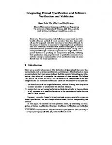
3.2 Description A brief overview of some of the grossest features of Petri nets in general have been described in x3.1; more detail, notation and examples speci c to CPNs will be discussed here. Consider Figure 3.4. Ellipses represent places, and rectangles represent transitions; line thicknesses have no special meaning other than to draw ones attention to particular features or relationships. Both places and transitions are labelled for identi cation. Special colour sets are de ned in a corner of the diagram, and standard ones are prede ned, e.g., N, Q, and R; every place also has its colour set speci ed. The quantities of tokens at each place are speci ed by the circled numbers next to the places | lack of such a number indicates no tokens currently mark that
33
Colour sets (p, i+1)
P = {e, f} x N
p ε P
R = {r}
i ε N
S = {s} 2
1‘(e, 0) + 1‘(f, 1)
P1
P
(p, i) s
Place labels 2‘r
T1 if p == e then (p, i) else NIL P2
P
Arc expressions 2 2‘s
r S
(p, i) if p == f then (p, i) else NIL
T2
[p == e]
3 R
(p, i) P3
P
3‘r
R
Markings/tokens
Guards if p == e then 3‘r else 2‘r
(p, i)
S
T3
Transition labels
Figure 3.4: A CPN diagrammed in Jensen's style.
34
s
place. The expressions next to the circled quantities, such as: 1`(e; 0) + 1`(f; 1);
(3.1)
represent the actual tokens present at the place; the number represents the number of tokens at the place with that speci c colour. So in Equation 3.1, there is one token of colour (e; 0) and one token of colour (f; 1); each is an element of the colour set P which itself is the Cartesian product of the nite set fe; f g with N. Arcs have a formal expression associated with them; the colour of tokens which then pass along an input arc of a transition may be referenced in expressions attached to the output arcs of a transition. Thus, in Figure 3.4, P1 is marked with one token of colour (e; 0) and one token of colour (f; 0), R is marked with three tokens of colour r and S is marked with two tokens of colour s. T1 is enabled since:
� P1 contains a token which conforms to the arc expression (p; i) where p 2 P and i 2 N, � R contains two tokens conforming to the arc expression 2`r, and � S contains a token conforming to the arc expression s. Arc expressions are good formal statements of the transformations performed upon tokens across a particular transition when it res, and are also easily displayed in diagrams; however, we will nd it more convenient to use an alternative formulation for our purposes: transition transforms . A transition transform describes the process of ring a particular transition as being the computation of a function of the transition's input tokens; the output tokens become the image of the input tokens under this transformation. The e�cacy of selecting the transition transform concept over that of arc expressions will be seen when we demonstrate that CPNs satisfy 35
our design goals for an integration environment, in x3.4. Guards are expressions a�ecting the behaviour of transitions; they are denoted in square brackets next to the transition they a�ect. A transition is enabled only if it meets both the standard requirements for enablement and its guard expressions evaluate to TRUE. The marking of Figure 3.4 may be denoted as:
9 8 >> P1 : 1`(e; 0) + 1`(f; 1); > > = < M0 = > R : 3`r; > > >: ;
S : 2`s The reachability tree may be displayed to a limited extent as in Figure 3.5; note that markings M00 and M000 are almost the same as M0 except that the second member of the token tuples for place P1 tend to increase, that is, they behave somewhat like counters. Thus, the basic behaviour of this marked CPN is fully illustrated by the given reachability tree. Jensen does not utilize inhibitor arcs in his standard formulation. Figure 5.1 demonstrates how to emulate an inhibitor arc in a CPN for a particular sub-net. Figure 3.6 depicts a marked generalized Petri net which is equivalent to the marked CPN of Figure 3.4. A general method of translation has been proven and is illustrated by Jensen [jens92].
3.3 Analysis Traditionally, the only reason Petri nets were deemed useful was that they could be analyzed to determine particular properties. Analysis has been the central focus of the model since not long after it was rst conceived. Any implementation of Petri nets, whether as a modelling tool or as a computational engine, should either take direct advantage of these analytical tools or permit another, higher software level, 36
8 P1 : 1`(e; 0) + 1`(f; 1); 9 = < M0 = : R : 3`r; ; S : 2`s T1 .
& T1
8> P1 : 1`(e; 0); 9 < R : 1`r; > = M1 = > S : 1`s; > : P3 : 1`(f; 1) ;
8 9 P1 : 1`(f; 1); > > < R : 1`r; = M2 = > S : 1`s; > : P2 : 1`(e; 0) ;
T3 #
T2 #
8 P1 : 1`(f; 1); 9 = < M2 = : S : 1`s; ; P3 : 1`(e; 0)
8 P1 : 1`(e; 0) + 1`(f; 2); 9 = < 0 M0 = : R : 3`r; ; S : 2`s
T3 #
8 9 P1 : 1`(e; 1) + 1`(f; 1); = < M000 = : R : 3`r; ; S : 2`s Figure 3.5: The reachability tree for the marked CPN of Figure 3.4.
37
Pf1
2
R
Pe1
2
4
4 Pe2
Pf3 2 4
4
S 5 3
Pe3
I1 5
I2
Figure 3.6: A marked generalized Petri net equivalent to the marked CPN in Figure 3.4, page 34.
38
such as an editor or modeller (e.g., [bill88]), to do so . This work will take the latter approach. Additional details of analyzing Petri nets will not be covered here; the interested reader is directed to Kurt Jensen's books on CPNs [jens92, jens95]. However, an overview of some of the concepts is in order. There are speci c properties that are of interest to modellers which are the focus of attempts at analysis.
Boundedness A net which never has more than k tokens at any place at a time is called k-bounded, and a net which is 1-bounded is termed safe . Obviously, all ordinary Petri nets are safe, since no place may contain more than one token at a time by de nition.
Conservativeness A net in which places always possess the same number of tokens before and after every ring is conservative ; this is important in systems in which tokens represent resources.
Deadness and liveness A transition is dead in a marking if there exists no reachable marking for which it is enabled; it is potentially rable if such a marking does exist, and is live if it is potentially rable in all reachable markings. The entire net is said to be live with respect to a particular marking if it is possible to re any transition in the net.
Deadlock If there exists a reachable marking from the initial marking such that no transitions are enabled, the net is said to be deadlock.
Mutual exclusion In some systems, no two processes should have concurrent access to the same resources.
Reachability It may be necessary to know all reachable markings in the net. 39
Reversibility If, for every reachable marking M from the initial marking M0, M0 is also reachable from M , we say that the net is reversible, i.e., the initial state can always be recovered. The standard techniques used to determine some of these properties include analysis of the reachability tree and invariant analysis. Construction of the reachability tree is straightforward, as immediately reachable markings branch out from the initial state. Since Petri nets can and often do represent an in nite number of states, there are two tricks for reducing the tree to a nite set of markings: if a marking is repeated, the branch is terminated; growing cycles where an in nite number of tokens accumulate at a place are also removable, see [pete77] for example. Of course, these two tricks are often insu�cient to maintain a manageable set of states, especially in higher-level nets, and much work has gone into reducing the size of the set, such as modular analysis where the pieces of a net are analyzed and the properties of the whole are deduced from the parts [jens92, chri92]. Invariant analysis seeks to nd equations which are satis ed by all reachable markings, in the case of CPNs, and sets of places whose number of tokens are invariant for all reachable markings, in the case of generalized Petri nets. In generalized (or ordinary) Petri nets, place invariants are determined by a linear algebraic means on the incidence matrix of the net. This matrix, A, is de ned as A = [aij ] where
aij = a+ij ? a?ij . a+ij is the number of arcs from transition j to place i and a?ij is the number of arcs from place i to transition j . Then solutions to the system A � y = 05 such that they cannot be additively obtained from other solutions are called invariants. If each place is in an invariant and the net starts with a bounded marking, the net is bounded, for example. 5
where yi 2 f0; 1g for ordinary nets, and y 2 N for generalized nets
40
Invariant analysis comes in two forms for CPNs and some other high-level nets: that of place invariants and that of transition invariants . The use and calculation of these are described by Jensen [jens92].
3.4 Satisfaction of Design Goals Pre-existing software packages can be accommodated in our conception of the CPN meta-model as the transition transforms without requiring any re-implementation. The internal computation of the transition transforms may be isolated from analyzing the rest of the behaviour of the net. CPNs, being a graph-like structure, obviously are well-accommodating to any highly non-planar interconnectivity scheme for communication. One might realize that ordinary (or generalized) Petri nets su�er from one feature which makes them impractical as anything other than a formalism: their component structures are so primitive that a truly huge net would need to be constructed for all but the simplest of functionality. Regardless of whether an \e�cient" method could be found to implement them as a computational engine, programmers would have di�culty with constructing and managing huge collections of nodes and their interconnections, thereby violating software engineering principles. A hierarchical structure, in which small subnets could be constructed for simple operations, then larger subnets could be constructed from these, and so on, would still be feasible; however, the ordinary (or generalized) Petri net formulation would not allow simple inclusion of existing software packages, which would then need to be reimplemented in terms of Petri nets. CPNs do not su�er from this de ciency: a transition transform may be arbitrarily complex6 | and this is where and how this 6
reminiscent of macrotransitions of [lee-87]
41
work proposes to integrate the existing systems. CPNs do not inherently require nor deny the ability to compute in a distributed fashion, thus, the possibility of distributed computing will be an implementation-level task. Petri nets in general were investigated because of their abilities to deal easily with the problems of concurrency and con ict [ramc74] which arise both in the context of distributed computing [vaut87] and of integrating simulation and animation software systems. Also, it has been recognized that \Petri nets are particularly valuable when state and control information are distributed throughout the system" [desr89]. The implementation will also be required to permit a hierarchical construction scheme for building-up increasingly complex and re ned subnets. Theoretical approaches to analyzing and treatment of hierarchical CPNs have already been investigated [jens92, chri92, buch93]. Such a hierarchical construction scheme, in combination with the integratability of existing packages, allow CPNs to be highly extensible. Strong typing and e�ciency are purely implementation-level tasks for CPNs. Later chapters will deal with these issues. A knowledgeable reader might question the e�cacy of utilizing the CPN model as a basis for ASCS in light of the existence of the interval timed coloured Petri net (ITCPN) model [aals93]. One must realize, however, that ITCPNs are a specialized model for the behaviour of the net itself, and not of its transition transforms; this work is not concerned with the behaviour of the net except as it a�ects the goals outlined in x1.4. Lakos has recently introduced a fully object-oriented version of CPNs as object Petri nets (OPNs) [lako95]. OPNs do capture the avour of the implementation 42
outlined in this work, perhaps better than CPNs do. These need investigation to see if the implementation requires modi cation to take advantage of any features unique to OPNs, and if the OPN model itself could be further re ned as was done herein to CPNs.
Summary Coloured Petri nets are a formalism used to describe complicated, concurrent and intercommunicating systems in a graphical fashion. They are heavily studied, and many analytical tools for them have been developed. They explicitly satisfy many of the design goals for an integration environment, and as such provide a strong basis for the construction of ASCS.
43
Chapter 4
Constructing ASCS via CPNs We have demonstrated that coloured Petri nets ful ll many of our design goals for an integration environment even without a speci c format for implementation. CPNs are relatively lacking in specialized support for the task we require: a meta-model for an integration environment. ASCS does provide this support, however; thus, we need the means for describing ASCS control graphs as CPNs.
4.1 Primitive Nodes As explained in x3.1, CPNs are Turing-complete. Furthermore, they possess only two classes of nodes: places and transitions. Any instance of either class may have 0 or more inputs and outputs, each with an arbitrary colour. The behaviour of a node with many inputs and/or outputs in general cannot be simulated by a succession of nodes of lower degree, or by a set of parallel nodes. Thus, there are an in nite number of primitive nodes, each with a di�ering in- or out-degree. But the situation is even worse, since each of these types is further di�erentiated on the basis of the colour set of each input or output, and colour sets may be collection classes. 44
Fortunately, the speci cation of any particular type of node is not recursive, so as long as we can construct a speci c type on demand, we do not need to be concerned about in nities. In fact, there is some programming language support for such parameterized classes.1 T
T (a)
T (b)
T (c)
(e)
(f)
(h)
T
(d)
(g)
(i)
T (j)
T (k)
T (l)
(m)
Figure 4.1: Symbols used in ASCS/CPN diagrams. Now, to allow the conversion of ASCS graph descriptions to CPN descriptions, and vice versa, we must specify CPN primitive nodes in terms of ASCS nodes, 1
Templates in C++, for example.
45
complete with binding sites. Figure 4.1 shows the basic symbols which will be used in ASCS/CPN diagrams: (a) - (d) represent binding sites | two binding sites may bind only if they are of the same colour class, di�erent shape, and same ll pattern; (a) is a place output binding site; (b) is a transition input binding site; (c) is a transition output binding site; (d) is a place input binding site; (e) represents the boundary of a node; (f) will contain an internal variable for a node2 ; (g) is a token; (h) and (i) represent the transition and place primitives, respectively; (j) - (m) are inhibitor binding sites and test binding sites, to be discussed in later chapters.
Figure 4.2: An example of an ASCS/CPN diagram. The lower diagram is a compound node constructed as shown in the higher one; note the self-binding of the internal node. 2 Internal variables are only present in ASCS nodes which are not fully expanded as coloured Petri sub-nets.
46
A
T
U
T{ }
B
D C
Figure 4.3: Primitive ASCS nodes: a transition node on the left, and a place node on the right. ASCS nodes will be represented as a dotted boundary in which are embedded binding sites; these binding sites will be connected, internal to the ASCS node, to CPN nodes via arcs (see Figure 4.2). These arcs represent half of the directed arc which would be present in the corresponding CPN diagram if the binding site were bound to another binding site. Intra-node arcs represent complete directed arcs. Note that directed arcs cross the ASCS node boundaries only at binding sites. The primitive ASCS nodes (see Figure 4.3) will simply encapsulate the primitive CPN nodes.
4.2 Control Graph Components 4.2.1 Channels Figure 4.4 illustrates the ASCS/CPN equivalent to an ASCS channel. Note that place P2 is instantiated with a token | a token of the colour set QUEUE, which is a collection class parameterized by the Cartesian product TIME �DATA. A channel constructed as shown would have an arbitrary capacity: the channel 47
TIME x DATA
td TIME x DATA P1 td q q
P2 QUEUE
[!Full( q )]
[!Empty( q )]
T1 Rem( q )
T2
Enqueue( td, q ) Dequeue( q ) P3 TIME x DATA td
TIME x DATA
Figure 4.4: An ASCS/CPN channel. would block its input only if the queue had a maximum capacity, and would block its output only if the queue were empty; this is guaranteed by the guards. The actual capacity of the channel could be controlled by the particular form of queue used: a static queue could have a xed capacity, while a dynamic queue's capacity would be solely dependent on the availability of dynamic memory. The channel's operation begins when an ASCS node writes data across the input binding site to place P1. If the QUEUE token at P2 is not \Full", the transition T1 may re, thereby enqueueing the input token identi ed as td into the queue q and returning the result to P2. The second half of the channel operates symmetrically: as long as the queue at P2 is not \Empty", transition T2 may re, thereby dequeueing a token of the colour set TIME �DATA to be placed in place P3, and returning the remainder of the queue to P2. Another ASCS node connected to the output binding site may then extract the token from P3. It should be noted that in the standard formulation of CPNs, there is no 48
reason to suppose that the tokens will be removed from the channel in the same order in which they entered, because tokens could \pile up" in both P1 and P3, and these tokens could then be removed in any arbitrary order; the structure of a channel would need signi cant alteration in such a situation if we wished to maintain rst-in rst-out ordering, most likely involving the use of inhibitor arcs. However, this situation is eliminated if places can contain only a single token at a time. And this is the formulation of CPNs which will be suggested in later chapters, albeit for the purposes of easier implementation. TIME x DATA
td T1 td TIME x DATA
P1 td
td s P2
TIME x DATA
T2
T3 td
td s T4 s
TIME x DATA
Figure 4.5: An ASCS/CPN equivalent to an ASCS overwriting channel. An alternative to a queueing channel is an overwriting channel | one that replaces the currently held value with the newly input value. Figure 4.5 illustrates the ASCS/CPN equivalent of just such a channel. If there is no currently held value, transition T3 will simply store the input value; if there is a currently held value, transition T2 will overwrite the currently held value. If the output place for transition T4 is unmarked and place P2 holds a token, T4 will simply transfer that token to its output. 49
4.2.2 Control Flow Operators TIME x DATA
( t, d )
( u, e ) TIME x DATA T1
P1
( u, e ) if Clip( t, u ) != NIL then ( Clip( t, u ), d ) else NIL TIME x DATA
Figure 4.6: An ASCS/CPN gate node. Figure 4.6 illustrates the ASCS/CPN equivalent to an ASCS gate. Note that place P1 is initialized with a token upon the instantiation of the node: this contains the interval to which clipping will take place. Whenever the place connected to the input binding site is marked, transition T1 may re, thereby removing that token as (t; d) and the token from P1 as (u; e). T1 will then clip t to u: only the portion of t which is contained within u will remain. If no such remainder exists, nothing will be written across the output binding site; otherwise, the clipped interval combined with d will be so written. Regardless, (u; e) is returned to P1. An ASCS conditional node is really a class of nodes: this class is parameterized by the decision function which the node computes. Figure 4.7 shows its ASCS/CPN equivalent as re ecting this fact. The decision function Func is initialized when the node is instantiated. When the place connected to the input binding site is marked with a token 50
TIME x DATA
( t, d )
T1
if !Func( t, d ) then ( t, d ) else NIL
if Func( t, d ) then ( t, d ) else NIL
TIME x DATA
true
false
TIME x DATA
Figure 4.7: An ASCS/CPN conditional node. as (t; d), transition T1 may re. The decision function is then computed on the token. If the result is TRUE, the token is written across the true output binding site, otherwise it id written across the false output binding site. Many di�erent types of ASCS splitter nodes are possible3 ; the particular one whose equivalent is shown in Figure 4.8 divides its input time interval into n equal sub-intervals. The places P1 and P2 are intially unmarked. When P1 is unmarked and the place connected across the interval input binding site is marked, the token (t; d) at this place is written to P1 by the ring of transition T1. Likewise, when P2 is unmarked and the place connected across the n input binding site is marked, the token (t; n) at this place is written to P2 by the
ring of transition T2. When P1, P2 and the place connected across the advance input binding site are marked, transition T3 may re. If the time interval t received from P1 is [ti ; to ), T3 will write the time interval [ti ; ti + t n?t ) to the place connected to the output o
3
e.g., one in which the step size is not xed
51
i
interval
TIME x DATA
TIME x DATA
n
TIME x DATA
advance
(t, d)
(t, n)
(t*, d)
T1
T2 if n < 1 then NIL else n
T3
t t
TIME
n
P1
N P2
if n - 1 == 0 then NIL else Tail( t, n )
( Head( t, n ), d )
if n - 1 == 0 then NIL else n - 1
TIME x DATA
Figure 4.8: An ASCS/CPN splitter node. binding site, in combination with the data value d received across the advance input binding site. In addition, T3 will also write tokens back to places P1 and P2 if and only if n is greater than 1. If n is equal to 1, then the subdivision of the input interval has been completed, and no tokens are written to P1 or P2, to allow for the next time interval and value for n to be input. But if n > 1, [ti + t ?n t ; to) is written to P1, and n ? 1 is written to P2. o
TIME x DATA unbounded
td
T1
td
unbounded TIME x DATA
Figure 4.9: An ASCS/CPN OR-junction node. 52
i
Figure 4.9 illustrates the ASCS/CPN equivalent of an ASCS OR-junction. It is simply facilitated by making the maximal cardinality of the input binding site unbounded. Thus, any number of places may connect to it, and the ring of transition T1 will arbitrarily select the token to be written across the output binding site from one of the marked places, if such a place exists.
4.2.3 Synchronization Operators Currently, the only explicit synchronization operator de ned by ASCS is the ANDjunction, whose ASCS/CPN equivalent is displayed in Figure 4.10. Transition T1 may re when the places connected across the input binding sites are both marked. Then it simply copies the token td from the input input binding site to the output binding site, discarding the token from the trigger input binding site. TIME x DATA
TIME x DATA
input
trigger
td
td*
T1
td
TIME x DATA
Figure 4.10: An ASCS/CPN AND-junction node.
53
4.2.4 Memory Operators TIME x DATA
td T1 td P1 TIME x DATA
td
td
P2
s T2
T3 s
td TIME x DATA
s
td P3
TIME x DATA td T4 td
TIME x DATA
Figure 4.11: An ASCS/CPN latch node. The ASCS/CPN equivalent of an ASCS latch node, as illustrated in Figure 4.11, is relatively complicated due to the fact that it requires two distinct execution threads: one for initialization, and one for post-initialization. All its places are initially unmarked. When the place connected across the input binding site becomes marked, transition T1 may re; this would result in place P1 becoming marked. Now if place P2 were unmarked, only transition T3 would be enabled and so, the input token td would be stored at both P2 and P3; then transition T4 could re, writing this token through the output binding site. However, if place P2 were marked, only transition T2 would be enabled; thus, the input token td would be discarded in favour of a copy of the stored token s which would be output via P3 and T4. 54
It should be noted that an alternate formulation of latch, and a potentially more useful one, would allow the internal storage to be reset. This would require a separate input binding site for the storage data to pass through, but would be quite similar internally to the presented latch formulation. TIME x DATA
td s TIME x DATA P1
T1
s s
TIME x DATA
Figure 4.12: An ASCS/CPN constant node. Figure 4.12 illustrates the ASCS/CPN equivalent of an ASCS constant node. The place P1 is initialized with its token upon the instantiation of the node. Whenever the place connected across the input binding site is marked, the transition T1 is enabled; its ring causes the token s stored at P1 to be copied to the place connected across the output binding site, and returned to P1. The input token td is discarded.
4.2.5 Computational Elements Figures 4.13 and 4.14 illustrate the ASCS/CPN equivalents of ASCS unary mathematical operator and binary mathematical operator nodes respectively. These are each a class of nodes parameterized by the particular mathematical function Func 55
they compute. TIME x DATA
( t, d )
T1
( t, Func( d ) )
TIME x DATA
Figure 4.13: An ASCS/CPN unary operator node. TIME x DATA
TIME x DATA
first
second
( t, d )
( u, e )
T1
( s, Func( d, e ) )
TIME x DATA
Figure 4.14: An ASCS/CPN binary operator node. In the unary operator, transition T1 is enabled when the place connected across the input binding site is marked by the token (t; d). When T1 res, it writes the computed Func(d) to the place connected to the output binding site, in conjunction with the input time interval t. 56
The binary operator is similar except that its transition T1 requires both of its input places to be marked before it is enabled, and it writes its computed Func(d; e) to its output place. Furthermore, so as not to bias the node in favour of one of its inputs, the output time interval is unde ned in the given formulation. TIME x DATA TIME x DATA
TIME x DATA
first
between second ( [u,u*), e ) ( [t,t*), d )
( [v,v*), f )
T1
u-v v-t ( [v,v*), d ____ + e ____ ) u-t u-t
TIME x DATA
Figure 4.15: An ASCS/CPN linear interpolator node. The operation of the ASCS/CPN equivalent of an ASCS linear interpolator node, illustrated in Figure 4.15, is straightforward, and indeed, could be implemented via more primitive operations. The tokens ([t; t� ); d) and ([u; u�); e) arriving over the rst and second input binding sites respectively have their values interpolated to determine a data value at time v , obtained via the between input binding site. The interpolated value of
d uu??vt + e uv??tt is written over the output binding site along with the time interval [v; v �).
57
4.2.6 Stewards Stewards are a widely varying class of node; all the details are di�cult to lay out without a precise framework for the implementation, which we have not discussed as yet. The deferral mechanism of ASCS may also cause problems to implement with a CPN | not because a CPN is incapable of simulating it4 , but because the process may become prohibitively expensive. One of the nice features which our implementation design for CPNs will exploit is the usually local nature of changes in a CPN: when a transition res, only the markings of the places to which it is connected will change. However, support of deferral will require near-global changes. When an actuator decides not to defer, all currently deferred actuators become undeferred, so the graph needs to control the state of all actuators in a centralized manner. In the next chapter, the concept of a register place will be introduced to decrease the cost of this feature. The actual usage of register places in deferral will be discussed in Chapter 6.
4.3 An Example Subgraph Figure 4.16 illustrates an ASCS subgraph to perform a primitive left-edge quadrature, and Figure 4.17 shows its ASCS/CPN equivalent5 . The interval over which to perform the quadrature will enter the subgraph via the input input binding site, requests for data values at particular times will exit the subgraph at the request output binding site, the responses to these requests will return to the subgraph via CPNs are Turing-complete, after all Some of the binding sites have been duplicated rather than attempt to show binding sites with binding cardinality > 1. 4
5
58
input
OR-junction0
td
0
constant0
OR-junction1
sum
td
add
response
sum
td
td
d
sum input
OR-junction2
constant1
trigger AND-junction td
n
d sum value
interval
n
td
advance
splitter
time time-tag
done finished
request
Figure 4.16: An ASCS subgraph to perform a primitive left-edge quadrature. the response input binding site, and the nal calculated quadrature will exit the subgraph at the nished output binding site. This formulation requires the speci cation of two additional types of ASCS nodes: a new form of splitter, and a time-tag node. The former is just like a traditional splitter save that when the entire interval has been subdivided, all additional advance signals cause the original interval is output via its done output binding site.
A time-tag node conjoins a given time interval and data value and writes them its output binding site. The subgraph operates as follows:
� an input time interval (and data value) arrive at the OR-junction0 node; � this value is copied, and written to the constant0, constant1, OR-junction2, and splitter nodes;
� both constant nodes then output their values: the constant0 node outputs a 59
OR-junction0
channel
constant0
channel OR-junction1
add channel
channel channel
channel
constant1
channel
o/w channel
OR-junction2 AND-junction
channel
channel
channel channel
splitter channel
time-tag
Figure 4.17: An ASCS/CPN equivalent to the ASCS subgraph in Figure 4.16. 0, the constant1 node outputs some predetermined n > 0;
� the OR-junction1 node passes the 0 from the constant0 node to the add node; � the OR-junction2 node passes td from the OR-junction0 node to the advance input binding site of the splitter node;
� the splitter node sends out the rst sub-interval via the request output binding site;
� the request value arrives at the response input binding site of the add node; � the add node sums the value received from the OR-junction1 node, which contains the running sum, and the new value received externally;
� this sum is then used both to trigger the next sub-interval request, and as the next input as the running sum via the OR-junction1 node; 60
TIME x DATA
t
interval
T2
t
(t, d*)
P1
P2
(u, d*) n TIME
TIME x DATA
if n < 1 then NIL else n
P3
(t, d*)
T1
T3
if n - 1 == 0 then NIL else Tail(t, n)
N
n (t, n) TIME x DATA
if n - 1 == 0 then NIL else n - 1
(t*, d) P4
advance (t*, d)
TIME x DATA
(t*, d) if n - 1 == 0 then (u, d) else NIL
TIME x DATA T4
( Head(t, n), d )
P5
(t*, d*) (t, d) T5
TIME x DATA (t, d)
done
TIME x DATA
current
TIME x DATA
Figure 4.18: An ASCS/CPN equivalent to the special ASCS splitter node used in the example subgraph.
� when the summation is complete, the splitter node releases the original interval via its done output channel; this triggers the AND-junction node to release the completed summation6 ;
� and nally, the time-tag node attaches the original input interval to the sum. Figure 4.18 illustrates the ASCS/CPN equivalent to the special ASCS splitter node used in the quadrature subgraph. Its basic operation is identical to the ASCS/CPN splitter node illustrated in Figure 4.8 on page 52. The chief di�erence is in its behaviour with regards to the advance input binding site when the inter6 This requires that the channel between the add node and the AND-junction node be overwriting rather than queueing; otherwise, the output value will be the rst sum calculated by the add node!
61
val has been fully sub-divided: at this stage, transition T3 writes the time interval initially received at the interval input binding site to place P5. When the next token is received across the advance input binding site, instead of writing the next sub-interval, the original interval is written out via the done output binding site by transition T5.
Summary ASCS may be simulated by CPNs. The problem of accommodating the deferral mechanism of ASCS remains to be discussed. A signi cant phenomenon occurs as one attempts to model a system with an abstract interface in ASCS/CPN. At rst, one may attempt to use primitive nodes to build up a macro-node to perform some task. Such collections of nodes can be relatively expensive to evaluate compared to other formulations such as machine code. Eventually, the abstraction may be great enough that cost savings can come about by replacing the internal mechanics of a high-level node with some specialized code, written in the language of choice. The ultimate expression of this is the principle of code re-use and large system-integration which is pivotal to this work.
62
Chapter 5
A Format for Implementation CPNs in and of themselves satisfy many of our design goals for supporting an integration environment such as ASCS1 ; the rest require speci c implementation support:
� distributed computing, � a hierarchical construction scheme, � strong typing, and � e�ciency. CPNs as de ned by Jensen [jens92] support all the basic features common to many variants plus guards2; additional features include:
� inhibitor arcs [chri93]3; � test arcs, which are an \alternative" to guards [chri93]4; see xx1.4, 2.4, and 3.4 described in x3.2 3 Inhibitor arcs will be discussed in x5.1. 4 Test arcs and guards will be discussed in x5.2. 1 2
63
� prioritizing the transitions, to decide ties in enablement [ajmo87]5; and � place capacities [chri93]. Also, there are three possible situations we can take into account in implementing an ASCS/CPN environment: 1. a single-processor system, 2. a multi-processor, non-distributed system, and 3. a distributed system. Each will be described as to its e�ects on e�ciency and behaviour of an ASCS/CPN environment.
5.1 Inhibitor Arcs As previously described in x3.1, inhibitor arcs are analogous to a logical NOT operation: the transition to which an inhibitor arc is connected is enabled only if the place to which that arc is connected is unmarked. As Figure 5.1 demonstrates, explicit support of inhibitor arcs is not necessary in the CPN domain; however, this diagram also illustrates the fact that, should inhibitor arcs not be supported, simulating them can add greatly to the complexity of the structure of the net. Basically, for a place which needs to inhibit any transitions, a second place is needed which acts as the indicator for \my partner is empty" | for example, it could store a count of the number of tokens in that place in a multi-token CPN domain. Thus, any transition which is connected to that place must also be connected to the second place. In a CPN domain with unitary place capacities, the 5
Prioritization will be discussed in detail in x5.4.
64
T!
T2 P P!
T5
T3
T4
T!
T2
P
N
P1
T5 PInh1
T3
T4
Figure 5.1: An example of equivalent CPNs with and without inhibitor arcs. simulation could be implemented such that when a token is written to one of these places, it is removed from the other. Increasing structural complexity is of concern because: 1. net evaluation cost may depend upon the size of the net, 2. it is more likely to lead to errors in design, and 3. it will increase the cost of analyzing the net. Thus, if inhibitor arcs may be supported cheaply, they should be.
65
5.2 Test Arcs and Guards Test arcs are decision functions which act upon a single place in determining whether or not a transition is enabled. However, not all functions may be computed as logical ANDs, so either multi-arcs6 or guards are required. A guard may be implemented as a set of test arcs and a single associated decision function. One simple task a guard easily handles which is beyond the capabilities of simple test arcs alone is deciding if the tokens in two places are equal. Heretofore, the term test arc will be used as specifying an input to a guard. The consequences of supporting guards in an implementation will be shown to be signi cant in the following sections.
5.3 Enablement The only dynamic factor within a net which determines its operation is the ring of transitions7 . Since ring is controlled chie y by the enablement of a transition, the means by which enablement is controlled and/or determined will be one of the greatest factors in determining the e�ciency of any implementation of CPNs. An implementation of Petri nets may be compiled or interpreted, sequential or concurrent, centralized or distributed, and synchronous or asynchronous [briz94]. We will look at simpli ed categorization in terms of number and distribution of processors. Also, we must choose between having the implementation being place-driven, in which a particular place is selected, and one of its transitions is selected to re, or transition-driven, in which places are passive. A place cannot be characterized 6 7
arcs which sweep across multiple places Non-static connectivity will be discussed in x6.3.3.
66
by its enabled transitions as easily as the transitions themselves could be [briz94]; it will be shown in x5.3.1 that place-driven schemes will not permit the use of the enablement bookkeeping method to be discussed there.
5.3.1 An Enablement Bookkeeping Method Consider there being an integer variable associated with each transition in a CPN called its enablement. When this variable attains the value 0, it indicates that the transition is enabled; otherwise, it is disabled. We require a means to update these values for all the transitions in a marked net every time a transition res. All the places in a CPN can be partitioned, relative to a particular transition, into one of ve categories8:
� an input-only place, � an output-only place, � an input-output place, � an inhibiting place, or � an unconnected place. A transition is enabled if all its input places and input-output places are marked, and all its output places and inhibiting places are unmarked, otherwise it is disabled. Thus, the enablement of a transition alters only when the marking of one of its associated places changes. Then if 1 is added to the enablement for each place which is not in the proper state to enable that transition, the enablement becomes a useful computational measure. 8
We have demonstrated this in Theorem 8 in Appendix B.
67
After a transition res, each place which goes from being unmarked to being marked subtracts 1 from the enablement of each of its associated transitions for which it is
� an output-only place, or � an inhibiting place and adds 1 to the enablement of each of its associated transitions for which it is
� an input-only place, or � an input-output place. Unconnected places and places which either remain unmarked or remain marked do not have their enablements altered. The operation of a place going from marked to unmarked is the opposite to this. If guards are to have their operation rolled into this bookkeeping scheme, everything stated above remains true with some additions. Each guard is marked as enabling or disabling according to the previous test performed via that guard. For every transition testing a place whose marking changes, a place which becomes marked, or a place which becomes unmarked, the test for that guard is repeated. Let an enabling decision be denoted as 1, and a disabling decision be denoted as 0. Then the associated transition has added to its enablement the new state of the guard minus the previous state of the guard, and the guard's state is updated. The updates can be performed in constant time, so the only expense is the cost of computing the decision function itself. Now, as long as the enablements (and guard states) were initialized correctly for the initial marking, transitions will be enabled if and only if their enablement variables contain the value 0. 68
Linear enabling functions (LEFs) [briz94] are a similar concept, but our model was developed independently. This work takes advantage of the special formulation of CPNs used herein to greatly reduce the number of classes needed by LEFs. Also, LEFs classify transitions whereas this enablement bookkeeping method classi es places relative to each transition.
5.3.2 Single-processor System A multi-threaded system is a waste of resources in a single-processor setup, since more overhead in terms of memory and computing time will be required, without increasing the net amount of computation.9 There are three ways in which enablement could be determined: on-the- y, via lazy evaluation, and via continuous update.
On-the-Fly In this scheme, after the initial marking is set or a new marking is computed, a scan would need to be made by the scheduler throughout the net for an enabled transition to re. This scan would consist of locating a transition, checking each of its input and output places for their marking, and possibly performing tests upon the tokens it nds there. Such a procedure would require that the scheduler have access to a list of the transitions, which would ensure that each was visited and only visited once, and that each transition possess a list of its input places and another of its output places. Every time a transition were eliminated as being disabled the next could be found in constant time. Of course, this fact would likely be secondary to time constraints in a real-time system, but this is beyond the scope of this work. 9
69
Another possibility is to allow the scheduler direct access to only one transition, and force it to follow arcs to nd the next transition. So let us start at transition T1 which is disabled; the scheduler marks it as disabled and begins to check its neighbours. Let us assume that it scans rst the input places and then the output places of that transition; for each of these places, the scheduler scans rst the input transitions, and then the output transitions. Unless the graph connectivity is of very low degree, the same transitions will tend to be visited repeatedly, two pointers will have to be dereferenced to locate the next transition, every transition will need a 1-bit ag to indicate whether it has been visited, and every one of these transitions will have to be visited again to turn the ag o�. Alternatively, the scheduler could keep an ordered record of which transitions had been visited, but insertion of this information would take (log v ) operations, and searching it would require O(log v ) operations on average, where v is the number of transitions already visited. A third alternative for the follow-the-graph approach would be to maintain a counter for each transition to indicate if it had been visited. When each search begins, the global counter would be incremented. As each transition is encountered, its local counter would be compared to the global one; if it were equal it would be assumed that the transition had already been visited on this search. Otherwise, the transition's counter would be set to the value of the global counter to indicate that it had been visited. But this will simply reduce the number of required scans per search from two to one, rather than altering the complexity. Thus, maintaining a list of transitions would be more e�cient, in terms of time, over the double-pass graph search and, in terms of both time and space, over the search-and-record method. The best-case scenario is one in which the rst transition encountered is enabled, thus rendering further search unnecessary. Furthermore, this transition 70
should have a minimal number of places connected to it, and be linked to none via test arcs. Assuming that checking for the presence of a token could be accomplished in constant time, this would also require constant time. Now, let each of the t transitions in the net be connected to each of the
p places, and also let each be linked to every place by a test arc. Assume that every transition were actually disabled, but that this is due solely to the decision computed by the nal test arc checked for each transition. Furthermore, assume that the computation of a guard's decision requires c operations for each of its test arcs. Then the worst case will require tp + tpc time. Assume that a transition is connected to dT places on average, that the average number of test arcs incident upon a transition is a, that one would need to test � percent of the transitions on average to nd one that was enabled, and that
percent of the test arcs needed to be tested on average. Then the average case would require �tdT + �t ac + ac operations, which is in O(tp + tpc).
Lazy Evaluation There are two approaches to this scheme, each treating test arcs di�erently; however, each treats enablement in terms of connected places identically. The idea takes advantage of the fact that the change in enablement from a marking to an immediately reachable marking is fairly local | only the input and output places of the red transition have their markings altered, and thus, the enablement of only the transitions which are either connected to these places or which test these places change. So given that there is some way to keep track of whether such a change alters the enablement of a transition without having to
71
recheck all of the unchanged places10 , it may be possible to reap a computational bene t. Such a scheme is possible and the cost of updating the net's bookkeeping after ring a transition is dT dP on average, where dT is the average number of places connected to a transition, and dP is the average number of transitions connected to a place. Then if �� percent of the transitions needed to be tested, the total cost of ring would be �� t + dT dP + �� t ac + ac operations, which is in O(t + tp + tpc). If test arc enablement were rolled into the bookkeeping scheme, updating the bookkeeping would cost dT dP + dT aP c, where aP is the average number of test arcs connected to a place. Then the total cost would be �� t + dT dP + dT aP c, which is in O(t + tp + tpc). In an \average net", connectivity will be fairly low since they are designed by humans11, and the more interconnected they are, the harder they would be to design; the number of enabled transitions could vary from many to few. Also, few test arcs are likely in an average net. Thus, rolling test arc enablement into the bookkeeping is likely to be more e�cient although there is no way to prove this. Once again, the best case is where the rst transition encountered is enabled, and that it has only one directed arc, and no test arcs associated with it. Then the cost of determining a rable transition is constant. The cost of the bookkeeping would also be constant12 if, for example, the transitions were all connected linearly. Thus, the total cost would be constant. The worst case remains that described under the on-the- y scheme: updating will cost tp so the total cost becomes 2tp + tpc which is still in O(tp + tpc). Such a method is outlined in x5.3.1. Humans will tend to design simple components and build them up to perform a complicated operation, even though a much denser CPN might perform the same operation. ASCS will also build somewhat redundancy- lled CPNs since humans will be designing all the components for use. 12 This is shown in x5.3.1. 10
11
72
Continuous Update This scheme is identical to lazy evaluation in terms of the bookkeeping. The di�erence lies in the fact that no scanning is required; instead, two queues of transitions will be maintained: one with enabled transitions, the other with disabled transitions. A doubly-linked queue will be required, however, as items from the middle of the queue must be removable. Enqueueing, dequeueing, and \de-splicing" are all
O(1) operations. Therefore, all we have is the cost of the bookkeeping to consider, so the average cost will be dT dP + dT aP c, the best case cost will be constant, and the worst case cost is tp + tpc.
5.3.3 Multi-processor, Non-distributed System The simplest way to utilize a multi-processor system would be to use a single processor to determine enablement and scheduling transitions, and use the other processors only to parallelize the computation of the transition transforms. This is likely to be very e�cient if the transition transforms themselves are very expensive and are parallelizable, since more than one transition could presumably be red at a time. A more likely scenario is to permit parallelization of separate transition transform computations; this requires a signi cantly di�erent approach from that of a single-processor system (x5.3.2). Consider an analogy between a CPN and a multiprocess operating system: transitions are processes, while places are shared memory. Thus, we will require a means to ensure mutually-exclusive shared memory access, and a scheduler for the allocation of processors to enabled transitions. Furthermore, an additional enfolding of the enablement bookkeeping system, this time with the mutual exclusion mechanism, would be ideal if it is possible as it should reduce 73
costs. Such an enfolding is eminently possible if mutual exclusion were implemented with semaphores [dijk65] given that they involve incrementing and decrementing a counter, which is essentially all that is involved in the enablement bookkeeping. Now, the scheduler could act as a centralized controller, as in the singleprocessor system, with the transitions acting as passive elements, or the transitions themselves could be self-coordinating. The latter would essentially be an operating system unto itself. A potential problem arises in the area of deadlock due to two or more transitions, each with access to part of their connected places, waiting for the other transitions to surrender the remainder. This indicates a need for acquiring and freeing place locks in a complete block. An algorithm such as that of Ricart and Agrawala [rica81, rayn88] could be used. In this algorithm, a transition13 which wishes to re must obtain exclusive access to each of its input and output places. Messages are sent o� to all the other transitions in the net, and access to a set of places is eventually granted. They showed that, if there were t transitions in a net,
t messages would need to be sent to obtain access. The total cost of locating a transition for ring would then be mt + dT dP + dT aP c, if readying, sending and processing a message required time m, assuming the continuous update method were utilized. If each transition were given knowledge of local graph connectivity, the Ricart and Agrawala approach might bene t since only those transitions which shared the places with a rable transition would have to be communicated with to obtain exclusive access. This was only a cursory examination of the available literature on multi13 Actually, the algorithm refers to processes, but we can easily see the analogy between transitions and processes | in fact, transitions could be implemented as processes.
74
threaded approaches. There may be other, better methods which are known, or the CPN realm might permit some new, special methods.
5.3.4 Distributed System In a truly distributed system, the cost of message passing quickly surpasses much of the local computational costs, so e�cient distributed algorithms need to minimize the number of messages. A CPN could be divided into sections with each running on an independent system. The centralized controller approach is easily implemented in this fashion. If the continuous update scheme were in place, an additional cost would be incurred of [mq + m� (1 ? q )]dT dP where q is the percentage of the transitions located on the local system and m� is the cost of readying, sending, and receiving a message across the network. Alternatively, the scheduler itself could be divided as well as the net. Separate sections of the net would no longer have any knowledge of each other. Arcs which bridge the network would require some form of proxying of their associated place to both sides of the network gap. Refer to Figure 5.2. The dashed line represents the machine boundaries; place P1 is connected across the network. On the right, P1� is e�ectively the proxy of P1 while the dotted arcs between the unnamed transitions are network connections. The implementation in the gure would still require some form of mutual exclusion in place since computation on either side of the network would be in parallel. The lazy evaluation approach holds greater promise here; it is reminiscent of the approach of Chiola and Ferscha [chio93] towards exploiting the structure of the net for e�ciency in a distributed implementation. A completely di�erent approach would be to subvert an election method such 75
T1
T1
P1
P1
P2 P1*
T2
P2
T2
Figure 5.2: The construction of a bridge across a network gap.
76
as the bully algorithm [silb93], or a ring-based election algorithm such as that of Chang and Roberts [chan79, tane92]. The former requires t2 messages, while the latter requires 3t ? 1 messages. However, these methods would only allow a single transition to re at a time, which is very wasteful of the large numbers of processors available. The Ricart and Agrawala approach of the previous section was actually developed for distributed mutual exclusion14 , so it would seem a good candidate, particularly the local connectivity variant. Of course, there is also the possibility of migrating processes, but such topics are beyond the scope of this work. Distributable nets were introduced by Hopkins [hopk91] to simulate a distributed implementation of a non-distributed system. Although potentially useful to this work as a starting point, a basic assumption made by Hopkins is that a transition's output places do not a�ect its enablement; thus, the model studied does not support inhibitor arcs, and as such is not Turing-complete.
5.4 Prioritizing Transitions P
T1
P
T2
0
T1
T2
1
Figure 5.3: Prioritized transitions In the diagram on the left of Figure 5.3, the selection of either transition T1 or T2 to re is arbitrary. With the addition of priorities in the diagram on the right, Recall that mutual exclusion is required so that multiple transitions do not simultaneously access the same place. 14
77
T1 has explicit priority to re. PR1 0
T1 T1
P2
P1
P2
P1 PR2
T2
1
T2
Figure 5.4: Equivalence of CPNs with and without priorities As illustrated in Figure 5.4, prioritizing transitions is not strictly necessary; however, it can simplify the construction of CPNs which possess a lot of explicit sequencing. In the diagram on the left, T1 has priority to re over T2. PR1 and PR2 are used to control the movement of a priority token; when T1 res, it either outputs to P2 or it returns the token to P1 and passes the priority token on to PR2. Many transitions could be connected to the priority places in this fashion just as many transitions could have the same priorities. Local sequencing of transitions can always be controlled in this fashion. It should be noted that if only local sequencing is required, construction of CPNs without prioritized transitions is not so di�cult. In the continuous update scheme, prioritization is straightforward: instead of two queues, 2n queues are used to model n di�erent priority levels. Each queue is checked in sequence until an enabled transition is found, which of course adds slightly to costs. Insertion of a transition is still of constant cost, but extraction will require some percentage of t on average since each queue needs to be checked for 78
occupancy | the precise average depends upon the net. Alternatively, a priority queue could be used. If such is implemented with a binary heap, the cost of insertion then rises to �(lg n), and extraction becomes the same (which may be an increase or a decrease) [corm90]. Mergeable heaps will have additional, useful properties if priorities are to be supported, as will become evident in x6.3.1. Fibonacci heaps [fred87] and relaxed heaps [dris88] permit insertion in constant amortized time and extraction in O(lg n) amortized (not amortized for relaxed heaps) time; relaxed heaps also have some advantages over Fibonacci heaps in parallel algorithms. However, direct support of prioritization will incur an extra cost regardless of the method of implementation. And as will be seen in x6.3.2, utilization of mergeable heaps does not permit cheap de-construction of nets. Thus, prioritization should be avoided to eliminate these extra costs, whenever possible.
5.5 CPN Re nements Utilized in This Work In this work, the following features will be supported:
� each place may hold either zero or one token; � inhibitor arcs; � guards, described as a set of test arcs plus a decision function; � transition transforms, as opposed to arc expressions; and � transitions have priorities, in an optional extended formulation.
79
Only single directed arcs, in each direction, and single inhibitor arcs are permitted between the same place and transition, since more would be redundant15 and would potentially increase costs. Only either directed arcs or inhibitor arcs are permitted to connect a particular place and transition, since having both is redundant16. Between a place and a transition, no more than one test arc is permitted due since a decision function should need to detect the value of the token just the once. Place capacities are limited to a single token for three reasons: 1. multiple tokens at a place may be mimicked by having a collection class as the colour set of that place, 2. this greatly simpli es the operation of ring, and 3. this does not impose a particular means of selecting among tokens when options are available | this is left up to the transition transform, reminiscent of a reduced instruction set chip (RISC) approach.
5.6 Related Work There have been many papers published concerning the implementation of Petri nets, in a single-processor system [vale86, colo87], a multi-processor non-distributed system [taub88, hein89, butl90], and a distributed system [brun86, colo87, bald88, sibe93, brun95]. Various implementations of CPNs exist [vale91, jens92, ba~na93], as do many tools for the use of Petri nets [feld93]. All are concerned with simulating the behaviour of a (coloured) Petri net, rather than using the Petri net formulation as a workhorse. Although these im15 16
This is proven by Theorems 2, 3, and 4 in Appendix B. as shown by Theorem 8 in Appendix B
80
plementations are often e�cient, they strive to maintain such awkward features as arc expressions. Arc expressions do not easily permit the insertion of pre-existing software in the same way that transition transforms do | the pre-existing software would need to be translated into a set of arc expressions, which is di�cult and counter-productive. The black box approach of transition transforms allows us to achieve our goals much more readily. There have even been Petri net implementations speci cally designed for simulation such as the Devnet [evan93] and the environment of Bastide and Palanque [bast95]. But these are strictly discrete event systems, and the problems with using discrete event systems as an integration environment were outlined in x1.5.
Summary An e�cient and unique means of utilizing the coloured Petri net formalism as a framework for the implementation of an integration environment has been found. The key to this implementation is the e�cient detection and selection of enabled transitions; a method for updating this information rapidly has been devised. Moving the environment to a distributed version requires more study, but presents no direct obstacles.
81
Chapter 6
Implementation Details It can clearly be seen by the most casual observer: : : | Far too many
Now that a theoretical means for implementation has been established, the details thereof need to be explained. The continuous update scheme for a singleprocessor system will be the basis for this speci cation. Also, although implementing CPNs does not require the use of a particular language, we used C++ to develop the concepts, and so the terminology used herein is in uenced by that found in C++.
6.1 Transitions To permit strong typing of transitions, they should be implemented in some fashion as a class parameterized by the colour sets of their individual input and output arcs. Transitions are characterized by the numbers and types of input and output types, and therefore, by their individual transition transforms. The trouble, then, is to create a parameterized class for transitions when such have variable numbers of 82
parameterizing classes. The solution is to create an abstract base class for transitions and provide polymorphic methods to perform the proper operations for the derived transition classes. What properties of transitions may be abstracted to such a base class? 1. All transitions are either enabled or disabled: methods are required to change this property from the base class. 2. The enablement of a transition will change when the tokens possessed by its attached places change: a method is required to potentially change the enablement of each of the transitions. 3. All transitions re when they are enabled, and the scheduler selects them to re: a method is required to re the transition without knowledge by the scheduler of the transition's type parameterizations. The solution to the latter is simple enough: the base class has a \ re" method which takes no arguments and has no body which is then overridden by the derived classes. Each derived class then worries about calling its particular type of transition transform appropriately. The tokens from each input place will be read, the transform will be calculated, and the tokens will be written to the appropriate output places. Transitions will not need to worry about their enablement: the acts of reading and writing will implicitly re-calculate this information.
6.2 Places Places will be responsible for re-calculation of the enablement of their associated transitions. This means that a place must be aware of the transitions to which it is 83
connected as well as the capacity in which it is connected to them. Thus, it must maintain four disjoint sets of transitions to which it is attached; two would actually su�ce1 , but this would make incremental connections within a net more di�cult (see x6.3.1). When a place is read from or written to, it must follow the algorithm for enablement bookkeeping as outlined in x5.3.1. Since the token written to an inputoutput place is not necessarily the same colour as the one read from that place, It is possible that a savings could be made for input-output places; rather than automatically updating the enablements of its transitions as soon as its token has been read, a searchable list could be set up containing these places. If the place was then written to by the same transition, a test could be performed to determine if the token had changed colour | if not, no enablement updates need be done. However, the cost of the overhead for such an elaborate scheme is likely to far outweigh the cost of two enablement updates, although it would depend on the connectivity of the place versus the number of input-output places for a particular transition. A special kind of place may be useful in the e�cient operation of a CPN engine, speci cally, instead of utilizing ordinary places with very high connectivity which tend to crop up when one tries to model the deferral mechanism of ASCS. We de ne a register place to be a place which is e�ectively connected to all the transitions of a subnet. It is always marked, and is assumed to always be enabling to these transitions, so no explicit changes to their enablement factors are required. 1
one for output-only and inhibiting, the other for input-only and input-output
84
6.3 Connections 6.3.1 Constructing CPNs For a full hierarchical construction scheme, a paradigm using an opaque interface which allows subnets to be treated in the same fashion as individual transitions and places will be required. To implement this, a somewhat di�erent view of nets will also be needed: the concept of binding sites from chemistry and biology will be used. The internal structure of a net will be opaque externally; all that other, non-friend classes will be able to see is that certain types of connections to other nets are permissible, and that only certain places may (or must) be initialized with tokens prior to net evaluation. Consider that places may only connect with transitions: a place may be thought of as a net with two binding sites, one for input and one for output, each of which can connect to an arbitrary number of transitions. Binding sites will have the following properties:
� maximal cardinality, � vertex type, � arc type, and � colour set. Maximal cardinality indicates the number of other sites which may be bound here, a positive integer or unlimited. Vertex type will be either place or transition. Arc type will be one of the following:
� input, 85
� output, � inhibiting, or � testing. And only binding sites with arc types input, output and testing will have di�erentiable colour sets, while all inhibiting types will have a single, unique colour set. There will also be marking initialization sites: only these places may have their markings initialized externally. Two sites may bind if they have opposite vertex types, identical arc types, identical colour sets, and the number of other sites already bound to each is less than their respective maximal cardinalities. Each subnet class will recursively tell its components how to connect down to the primitive transition and place nets. The names of the binding sites, and their properties such as maximal cardinality may be altered to suit the needs of the particular subnet. Each subnet is a CPN (or an agent whose interface to the rest of the graph is indistinguishable from a CPN) in and of itself: they should always be able to be evaluated. At rst glance, these arc types would seem to be at variance with the equivalence classes of places relative to a given transition. But it will be the responsibility of the primitive classes to ensure that the restrictions as outlined in x5.5 are respected, and that any place which becomes both an input and an output place for a transition is identi ed and classi ed as such. After connecting their components appropriately, two bound subnets must merge their respective queues of enabled and disabled transitions. If prioritization is supported, this is where mergeable heaps become most useful. After a subnet 86
has been fully connected to other parts of the completed net, the particular subnet may not be required any longer; thus, it should be possible to free some of the memory associated with the subnet while leaving the components intact and connected. Pointers will accomplish this, of course. Also, transition enablements must be updated whenever a new link is forged.
6.3.2 Deconstructing CPNs One might also wish to remove a subnet from a CPN | single transitions or places would be easy enough, but large chunks are more problematic. A CPN will possess a set of queues for its enabled and disabled transitions; presumably when two subnets are merged, these queues will also be merged, thus the identities of the vertices unique to the subnet will be lost. Furthermore, this in no way records the identities of the places associated with the subnet. Therefore, separate sets of pointers to transitions and places will need to be maintained for all extant subnets. When a subnet is to be removed from a CPN, its set of pointers is inspected and the corresponding transitions and places are removed from the queues; this can be quite expensive if prioritization is supported. However, such a form of removal will not maintain the various arcs within the subnet while removing the links to the other portions of the CPN. This is not a problem if the subnet is being discarded, but if it is to be moved to another position in the net, or to another net2, these arcs will be needed. Three basic approaches are then possible: 1. destroy all arcs connected to any vertex being removed and recreate the ones It is not clear under what such circumstances such a transfer operation would occur, but it would seem more desirable to move a pre-existing component than building an identical one up from scratch. 2
87
internal to the subnet, 2. check each arc to see if it is internal to the subnet by explicitly searching through the sets of internal vertices maintained by the subnet for each arc's other endpoint, or 3. also maintain a set of arcs. Scheme 1 promises to be ine�cient. Scheme 2 would require each subnet's internal sets to be searchable, which would mean that the operation of linking two binding sites together would get more expensive as subnets increase in size. Scheme 3 has potential, but would basically require that all arcs be true data structures; this would allow a set of pointers to the appropriate ones to be maintained. These questions are only really of signi cance when non-static connectivity is supported; further study of this topic is required.
6.3.3 Non-static Connectivity The question of adding vertices, removing them, and changing the arcs between them while a net is undergoing evaluation is an interesting one. Self-modifying nets have been studied in the context of non-coloured Petri nets [valk78], but it is unclear what a�ect this would have on the analytical properties of CPNs. In terms of simply evaluating a CPN, it is eminently doable: the system would simply need to ensure that, after ring a transition, each of its transitions were still fully connected before ring the next transition. This could be accomplished by maintaining a variable which records broken connections which is incremented when a connection is broken and decremented when one is established.
88
6.4 Graph Evaluation Graph evaluation will be performed by selecting an enabled transition: if priorities are supported, this transition will have the highest priority, i.e., least delay. Utilization of multiple queues or priority heaps will ensure that an enabled transition will always be selected if such exists. The simplest approach to selecting amongst the enabled transitions is simply to have a rst-in rst-out system | this has the added advantage of ensuring that starvation of an enabled transition will never occur. However, support of a feature such as deferral in ASCS is not so easily accomplished by this approach. Deferral, and \undeferral" by the system, would require that all of the transitions representing these dof access features in the stewards would need to be connected to central, \controlling" places. Whenever one of these nodes nally red, all the others would have to have their enablements changed, and moved from one queue to another, etc. This is potentially very expensive. An alternative method is to take advantage of register places (see x6.2) in combination with a di�erent selection method: allowing a selected transition to defer (by being moved to the back of the queue, or bottom of the heap). This could lead to deadlock since every enabled transition could continually defer3 , but this could be explicitly dealt with by not permitting more than x deferrals. This is the approach outlined in the following algorithm. Deferring-CPN Evaluation Algorithm
(0)
START: Places
have their initial markings installed.
(1) Calculate transition enablements. 3 This is not deadlock in the classical sense, perhaps, but it is e�ectively the same since each transition is waiting for another to do something.
89
(2) Initialize the state of each transition as UNDEFERRED. (3) Initialize the internal time of each transition to 0. (4) Insert transitions into appropriate queues or heaps. (5) Initialize the register place TIME to an initial time of 1. (6)
WHILE any
transitions are enabled, DO:
(6.0) Select an enabled transition from the head of the queue. (6.1)
IF
the internal time of the transition IS-LESS-THAN TIME, THEN:
(6.1.0) Set the internal time of the transition to TIME. (6.1.1) Set the transition's state to UNDEFERRED. (6.2)
IF
the transition defers, THEN:
(6.2.0)
IF
the transition's state is DOUBLY-DEFERRED, THEN:
(6.2.0.0) Force the transition to evaluate anyway. (6.2.0.1) Increment TIME. (6.2.1)
ELSE-IF the
transition's state is DEFERRED, THEN:
(6.2.1.0) Set the transition's state to DOUBLY-DEFERRED. (6.2.2)
ELSE-IF the
transition's state is UNDEFERRED, THEN:
(6.2.2.0) Set the transition's state to DEFERRED. (6.2.2.1) Copy TIME to the transition's internal time. (6.3)
ELSE:
(6.3.0) Increment TIME.
90
(7)
END: Cleanup.
The question of whether this is truly more e�cient than requiring implementation of this algorithm directly by the graph remains open, especially when taken in the context of distributed systems. Of course, the e�cacy of the deferral mechanism above any possible alternatives must itself be better demonstrated.
Summary Techniques for implementing CPNs in general and some speci c ones for the context of ASCS have been presented. The latter require further development especially considering their extension to the distributed purview. Better study and proof of the properties of ASCS may now take place given this means for formal de nition.
91
Chapter 7
Conclusion A speci cation for a generic computational engine has been presented. This engine has been shown to be of particular interest in the area of integrating simulation and animation software in a way hard to achieve at present. The means for implementing and analyzing coloured Petri nets as this computational engine are available, and the former have been given herein.
7.1 Summary Throughout this work, various problems were shown to exist, leading us from the need for integration to the implementation of ASCS as a CPN environment. The following is a summary of these assertions and their justi cations in this progression of concepts from initial problem to nal solution.
Assertion 1 Software manufacturers must specialize in the areas which their products concentrate upon, if they are to remain at the forefront of innovative research.
92
Justi cation The pace of research is exponential. Without specialization in a particular research area, a software package will become so unwieldy as to quickly become unmodi able and unmaintainable. �
Assertion 2 Designing a software package for modi cation can only partially accommodate future changes.
Justi cation The direction of research is unclear in the long-term. One would need clairvoyance to predict future advances | and to allow for their inclusion in a particular model. �
Assertion 3 Animators/simulators require products at the forefront of research. Justi cation If there were no need for these new products, there would be no need for further research. Although some of this is simply the novelty factor, the fact remains that this is the situation. �
Assertion 4 An animator/simulator may require any arbitrary software package at some point: this is Turing-completeness.
Justi cation This is a straightforward extension of Assertion 3. � Assertion 5 Combining the use of several of the specialized packages is the best way to take full advantage of the best features of each.
Justi cation If one package does not have all the bells and whistles required, but the combination of several individual packages does cover the spectrum, then integration is needed. �
Assertion 6 All but the simplest forms of interaction will require a true, concurrent sharing of models. In turn this necessitates con ict resolution between the disparate 93
packages as well as a scheme for coordinating their computations.
Justi cation If the form of coordination were so trivial, some manufacturer would have already provided it. For example, even within a large, single package like SoftImage, it is impossible to concurrently control the a�ect of two or more operations on a model; the internal workings of SoftImage will choose in what serial order the operations will occur. �
Assertion 7 Time makes for a good parameter for coordination. Justi cation Since we are attempting to make an animation or simulation | something which is inherently parameterized by time | time is obviously common ground for communication and thus coordination. �
Assertion 8 Di�ering notions of time among di�erent packages requires a special approach so as to accommodate all without temporal aliasing or any bias against a particular model.
Justi cation This is explained in Chapter 2. Fixed versus adaptive step size and continuous versus discrete events do not t well together, hence ASCS uses an interval representation of time. �
Assertion 9 The most general form of interconnection among a set of objects can be described as a graph.
Justi cation Any two of the objects can be unconnected, connected in one direction, or connected in both directions regardless of the other objects in the environment: all of these can be represented by a graph. �
Assertion 10 ASCS provides a su�cient environment for integration. 94
Justi cation ASCS is fully extensible. It is hierarchical, thereby providing simple macros for the most common of operations, while permitting the construction of unusual features from primitive functions. It provides a scheme for interaction, coordination, communication, and con ict resolution which is independent of a particular scheme for modelling time. �
Assertion 11 Coloured Petri nets are an e�ective engine for generic computation. Justi cation Transition transforms can accommodate an arbitrary piece of software, thereby allowing maximal code reuse with minimal extension. The graphical nature of CPNs allows for the most highly interconnected forms of communication that are required. Hierarchical construction allows data hiding of large, common macros, while providing Turing-complete functionality and extensibility. Parallel and distributed computation may be supported by CPNs as well. Furthermore, the properties of a system constructed from CPNs could be directly analyzed. �
Assertion 12 Coloured Petri nets can be implemented in an e�cient manner. Justi cation Determination of enabled transitions is the main factor in the speed of evaluating a CPN; an e�cient means of accounting for this has been shown. This requires O(dT dP + dT aP c) operations on average to update all the enablements in a CPN after a transition res, for a single processor environment. �
Assertion 13 ASCS can be e�ectively implemented with coloured Petri nets. Justi cation Coloured Petri nets meet all the criteria strictly required for ASCS plus a few more. The speci c form of the implementation will be partially dependent upon the nal form taken by ASCS: this is analogous to optimization, however. � 95
7.2 Future Work Further work needs to be performed in the area of a distributed implementation of coloured Petri nets, speci cally in terms of a thorough treatment of the possibilities and an analysis of the e�ciency of each. Failing this, experimental study should be pursued along these lines. The e�ects of self-modi cation to the analysis of CPNs needs study, as does a good tool for the analysis of the implementation of this work. Removal of subnets remains a signi cant problem in the context of self-modi cation. Object Petri nets (OPNs) [lako95] need investigation to see if the implementation requires modi cation to take advantage of any features unique to OPNs, and if the OPN model itself could be further re ned as was done herein to CPNs. The realm of multi-processor and distributed systems needs to be studied further; although the enablement bookkeeping method and continuous update scheme were shown to be e�ective and e�cient in a single-processor environment, the same is unlikely to be true elsewhere. Distributable nets [hopk91] also need to be more closely scrutinized for their use here. Constraint nets [zhan94] require some serious further study. It is possible that ultimately the goals of an ASCS-like environment can be comprehensively subsumed by a constraint-net-based system. At present, however, it must be remembered that Petri nets have undergone long-term and rigorous scrutiny; the tools for their analysis and usage are already in place. Constraint nets may not be su�ciently powerful in the range of problems which they may model, they may not permit the inclusion of pre-existing software packages without re-implementing them, and e�cient implementation of their programming semantics is still to be seen. Perhaps what will emerge in the end will be some child of both domains. 96
Bibliography [aals93] W. M. P. van der Aalst. \Interval timed coloured Petri nets and their analysis". In Ajmone Marsan [ajmo93], pp. 453{472. [ager73] T. Agerwala and M. Flynn. \Comments on Capabilities, Limitations and `Correctness' of Petri Nets". Proceedings of the 1st Annual Symposium on Computer Architecture, Vol. 1, pp. 81{86, 1973. [ajmo84] M. Ajmone Marsan, G. Balbo, and G. Conte. \A class of generalized stochastic Petri nets for the performance analysis of multiprocessor systems". ACM Transactions on Computer Systems, Vol. 2, No. 1, pp. 93{ 122, May 1984. [ajmo87] M. Ajmone Marsan, G. Balbo, G. Chiola, and G. Conte. \Generalized stochastic Petri nets revisited: random switches and priorities". Proceedings of the 1st International Workshop on Petri Nets and Performance Models, August 1987. [ajmo89] Marco Ajmone Marsan. \Stochastic Petri nets: an elementary introduction". In Rozenberg [roze89], pp. 1{29. [ajmo93] Marco Ajmone Marsan, editor. Application and Theory of Petri Nets 1993 (Proceedings of the 14th International Conference), Vol. 691 of Lecture Notes in Computer Science. Springer-Verlag, Berlin, Germany, 1993. [bald88] M. Baldassari and G. Bruno. \PROTOB: Object-oriented graphical modelling and programming based on Prot nets". In Rozenberg [roze88], pp. 333{342. [ba~na93] J. A. Ba~nares, P. R. Muro-Medrano, and J. L. Villarroel. \Taking advantages of temporal redundancy in high level Petri nets implementations". In Ajmone Marsan [ajmo93], pp. 32{48. 97
[bast95] R�emi Bastide and Philippe Palanque. \A Petri net based environment for the design of event-driven interfaces". In De Michelis and Diaz [de m95], pp. 66{83. [bill88]
J. Billington, G. Wheeler, and M. Wilbur-Ham. \Protean: A high-level Petri net tool for the speci cation and veri cation of communication protocols". IEEE Transactions on Software Engineering, Vol. 14, pp. 301{ 316, 1988.
[briz94] J. L. Briz and J. M. Colom. \Implementation of weighted place/transition nets based on linear enabling functions". Application and Theory of Petri Nets 1994 (Proceedings of the 15th International Conference), Vol. 815 of Lecture Notes in Computer Science, pp. 99{118. Springer-Verlag, Berlin, Germany, 1994. [brun86] G. Bruno and G. Marchetto. \Process-translatable Petri nets for the rapid prototyping of process control systems". IEEE Transactions on Software Engineering, Vol. 12, No. 2, pp. 346{357, February 1986. [brun95] G. Bruno, A. Castella, R. Agarwal, and M. P. Pescarmona. \CAB: an environment for developing concurrent application". In De Michelis and Diaz [de m95], pp. 141{160. [buch93] Peter Buchholz. \Hierarchies in colored GSPNs". In Ajmone Marsan [ajmo93], pp. 106{126. [butl90] B. Butler, R. Esser, and R. Mattmann. \A distributed simulator for high order Petri nets". Advances in Petri Nets 1990 (Proceedings of the 10th International Conference on Application and Theory of Petri Nets), Vol. 483 of Lecture Notes in Computer Science, pp. 22{34, 1990. [chan79] E. G. Chang and R. Roberts. \An improved algorithm for decentralized extrema- nding in circular con gurations of processors". Communications of the ACM, Vol. 22, No. 5, pp. 281{283, May 1979. [chio93] Giovanni Chiola and Alois Ferscha. \Distributed simulation of timed Petri nets: exploiting the net structure to obtain e�ciency". In Ajmone Marsan [ajmo93], pp. 146{165. [chmi91] M. Chmilar, B. Wyvill, and C. Herr. \A Software Architecture for Integrating Modeling with Kinematic and Dynamic Animation". The Visual Computer, Vol. 7, pp. 122{137, 1991. 98
[chri92] S�ren Christensen and Laure Petrucci. \Towards a modular analysis of coloured Petri nets". Application and Theory of Petri Nets 1992 (Proceedings of the 13th International Conference), Vol. 616 of Lecture Notes in Computer Science, pp. 113{133. Springer-Verlag, Berlin, Germany, 1992. [chri93] S�ren Christensen and Niels Damgaard Hansen. \Coloured Petri nets extended with place capacities, test arcs and inhibitor arcs". In Ajmone Marsan [ajmo93], pp. 186{205. [colo87] J. M. Colom, M. Silva, and J. L. Villarroel. \On software implementation of Petri nets and colored Petri nets using high-level concurrent languages". In Rozenberg [roze87], pp. 207{241. [corm90] Thomas H. Cormen, Charles E. Leierson, and Ronald L. Rivest. Introduction to Algorithms. McGraw-Hill Book Co., New York, NY, USA, 1990. [de m95] Giorgio De Michelis and Michel Diaz, editors. Application and Theory of Petri Nets 1995 (Proceedings of the 16th International Conference), Vol. 935 of Lecture Notes in Computer Science. Springer-Verlag, Berlin, Germany, 1995. [desr89] A. A. Desrochers. \Modeling and Control Using Petri Nets". Modeling and Control of Automated M/G Systems, tutorial 5. IEEE Computer Society Press, 1989. [dijk65] Edsger W. Dijkstra. \Cooperating sequential processes". Technical report, Technological University, Eindhoven, The Netherlands, 1965. [dris88] James R. Driscoll, Harold N. Gabow, Ruth Shrairman, and Robert E. Tarjan. \Relaxed heaps: an alternative to Fibonacci heaps with applications to parallel computation". Communications of the ACM, Vol. 31, No. 11, pp. 1343{1354, November 1988. [evan93] John B. Evans. \The Devnet: a Petri net for discrete event simulation". In Rozenberg [roze93], pp. 91{125. [feld93] Frits Feldbrugge. \Petri net tool overview 1992". In Rozenberg [roze93], pp. 169{209. [ sh88] Paul A. Fishwick. \The Role of Process Abstraction in Simulation". IEEE Transactions on Systems, Man and Cybernetics, Vol. 18, No. 1, pp. 18{39, January/February 1988. 99
[ um87] E. Fiume, D. Tsichritzis, and L. Dami. \A Temporal Scripting Language for Object-Oriented Animation". Proceedings of the European Computer Graphics Conference and Exhibition (EUROGRAPHICS '87), pp. 283{ 294, August 1987. [fred87] Michael L. Fredman and Robert E. Tarjan. \Fibonacci heaps and their uses in improved network optimization algorithms". Journal of the ACM, Vol. 34, No. 3, pp. 596{615, 1987. [genr81] H. J. Genrich and K. Lautenbach. \System modelling with high-level Petri nets". Theoretical Computer Science, Vol. 13, pp. 109{136. NorthHolland, Amsterdam, The Netherlands, 1981. [genr86] Hartmann J. Genrich. \Place/transition nets". Petri Nets: Central Models and Their Properties (Advances in Petri Nets 1986, Part I), Vol. 254 of Lecture Notes in Computer Science, pp. 224{247. Springer-Verlag, Berlin, Germany, 1986. [gett90] Phillip Getto and David Breen. \An Object-oriented Architecture for a Computer Animation System". The Visual Computer, Vol. 6, pp. 79{92, 1990. [hack74] M. H. Hack. \Decision problems for Petri nets and vector addition systems". Memo 94, Massachusetts Institute of Technology, Cambridge, MA, USA, March 1974. [haeb88] Paul E. Haeberli. \ConMan: A Visual Programming Language for Interactive Graphics". Computer Graphics, Vol. 22, No. 4, pp. 103{111, August 1988. [hein89] A. Heinrich and W. Ameling. \Multiprocessor system architecture for the execution of higher Petri nets". In Rozenberg [roze89], pp. 321{332. [holl85] M. A. Holliday and M. K. Vernon. \A generalized timed Petri net model for performance analysis". Proceedings of the International Workshop on Timed Petri Nets, pp. 181{190, July 1985. [hopk91] R. P. Hopkins. \Distributable nets". In Rozenberg [roze91a], pp. 161{187. [jens81] Kurt Jensen. \Coloured Petri nets and the invariant method". Theoretical Computer Science, Vol. 14, pp. 317{336. North-Holland, Amsterdam, The Netherlands, 1981. 100
[jens83] Kurt Jensen. \High-level Petri nets". Applications and Theory of Petri Nets, Vol. 66 of Informatik-Fachberichte, pp. 166{180. Springer-Verlag, Berlin, Germany, 1983. [jens92] Kurt Jensen. Coloured Petri Nets: Basic Concepts, Analysis Methods and Practical Use, Vol. 1 of EATCS Monographs on Theoretical Computer Science. Springer-Verlag, Berlin, Germany, 1992. [jens95] Kurt Jensen. Coloured Petri Nets: Basic Concepts, Analysis Methods and Practical Use, Vol. 2 of EATCS Monographs on Theoretical Computer Science. Springer-Verlag, Berlin, Germany, 1995. [kalr92] Devendra Kalra and Alan H. Barr. \Modeling with time and events in computer animation". Computer Graphics Forum (EUROGRAPHICS '92 Proceedings), Vol. 11, No. 3, pp. 45{58, September 1992. [kazm93] Rick Kazman. \HIDRA: An Architecture for Highly Dynamic Physically Based Multi-Agent Simulations". International Journal for Computer Simulation, 1993. [kuhn93] Volker Kuhn and Wolfgang Muller. \Advanced object-oriented methods and concepts fro simulations of multi-body systems". Journal of Visualization and Computer Animation, Vol. 4, pp. 95{111, 1993. [lako95] Charles Lakos. \From coloured Petri nets to object Petri nets". In De Michelis and Diaz [de m95], pp. 278{297. [lalo94] Paul Lalonde, Robert Walker, Jason Harrison, and David Forsey. \A Model for Coordinating Interacting Agents". Proceedings of Graphics Interface '94, pp. 149{156, May 1994. [lalo96] Paul Lalonde, Robert Walker, Jason Harrison, and David Forsey. \An architecture for coordinating kinematic and dynamic animation". Submitted to Journal of Visualization and Computer Animation , May 1996. [lee-87] Hyung Lee-Kwang, Joel Favrel, and Pierre Baptiste. \Gerneralized Petri Net Reduction Method". IEEE Transactions on Systems, Man and Cybernetics, Vol. 17, No. 2, pp. 297{303, March/April 1987. [lee94]
Gene S. Lee. \RASP: Robotics and Animation Simulation Platform". M.Sc. thesis, University of British Columbia, Vancouver, BC, Canada, January 1994. 101
[mcgr94] Donald R. McGregor and Sabah U. Randhawa. \ENTS: An Interactive Object-oriented System for Discrete Simulation Modeling". Journal of Object Oriented Programming, pp. 21{29, January 1994. [moll81] M. K. Molloy. On the integration of delay and throughput measures in distributed processing models. Ph.D. thesis, University of California at Los Angeles, Los Angeles, CA, USA, 1981. [mura89] T. Murata. \Petri nets: properties, analysis and applications". Proceedings of the IEEE, Vol. 77, No. 4, pp. 541{580, April 1989. [natk80] S. Natkin. Les reseaux de Petri stochastiques et leur application �a l'�evaluation des syst�emes informatiques. Th�ese de Docteur Ingegneur, CNAM, Paris, France, 1980. [over93] C. W. A. M. van Overveld. \Building Blocks for Goal-directed Motion". Journal of Visualization and Computer Animation, Vol. 4, pp. 233{250, 1993. [pete77] James L. Peterson. \Petri Nets". ACM Computing Surveys, Vol. 9, No. 3, pp. 223{252, September 1977. [petr62] Carl Adam Petri. Kommunikation mit Automaten. Ph.D. thesis, University of Bonn, Bonn, Germany, 1962. [ramc74] C. Ramchandani. \Analysis of asynchronous concurrent systems by timed Petri nets". Technical Report 120, Laboratory for Computer Science, Massachusetts Institute of Technology, Cambridge, MA, USA, 1974. [rayn88] Michel Raynal. Distributed Algorithms and Protocols. John Wiley & Sons, New York, NY, USA, 1988. [rica81] G. Ricart and A. K. Agrawala. \An optimal algorithm for mutual exclusion in computer networks". Communications of the ACM, Vol. 26, No. 1, pp. 9{17, January 1981. [roze87] Grzegorz Rozenberg, editor. Advances in Petri Nets 1987 (Proceedings of the 7th European Workshop on Application and Theory of Petri Nets), Vol. 266 of Lecture Notes in Computer Science. Springer-Verlag, Berlin, Germany, 1987. [roze88] Grzegorz Rozenberg, editor. Advances in Petri Nets 1988 (Proceedings of the 8th European Workshop on Application and Theory of Petri Nets), 102
Vol. 340 of Lecture Notes in Computer Science. Springer-Verlag, Berlin, Germany, 1988. [roze89] Grzegorz Rozenberg, editor. Advances in Petri Nets 1989 (Proceedings of the 9th International Conference on Application and Theory of Petri Nets), Vol. 424 of Lecture Notes in Computer Science. Springer-Verlag, Berlin, Germany, 1989. [roze91a] Grzegorz Rozenberg, editor. Advances in Petri Nets 1991 (Proceedings of the 11th International Conference on Application and Theory of Petri Nets), Vol. 524 of Lecture Notes in Computer Science. Springer-Verlag, Berlin, Germany, 1991. [roze91b] Gary D. Rozenblat and Richard R. Muntz. \The Tangram Simulation Animation System". Proceedings of the EUROGRAPHICS Workshop on Animation and Simulation, pp. 153{167, September 1991. [roze93] Grzegorz Rozenberg, editor. Advances in Petri Nets 1993 (Proceedings of the 12th International Conference on Application and Theory of Petri Nets), Vol. 674 of Lecture Notes in Computer Science. Springer-Verlag, Berlin, Germany, 1993. [sibe93] C. Sibertin-Blanc. \A client-server protocol for the composition of Petri nets". In Ajmone Marsan [ajmo93], pp. 377{396. [sifa77] J. Sifakis. \Use of Petri nets for performance evaluation". Measuring, Modelling and Evaluating Computer Systems, pp. 75{93. North-Holland, Amsterdam, The Netherlands, 1977. [silb93] Abraham Silberschatz, James L. Peterson, and Peter B. Galvin. Operating System Concepts. Addison-Wesley Publishing Co., Reading, MA, USA, fourth edition, 1993. [snyd92] John M. Snyder. \Interval Analysis for Computer Graphics". Computer Graphics, Vol. 26, No. 2, pp. 121{130, July 1992. [stei92] Je� S. Steinman. \SPEEDES: A Multiple-Synchronization Environment for Parallel Discrete-Event Simulation". International Journal for Computer Simulation, Vol. 2, No. 3, pp. 251{286, 1992. [stei94] Je� S. Steinman. \Discrete-Event Simulation and the Event Horizon". Proceedings of the 8th Workshop on Parallel and Distributed Simulation, 1994. 103
[tane92] Andrew S. Tanenbaum. Modern Operating Systems. Prentice Hall, Englewood Cli�s, NJ, USA, 1992. [tani94] Oryal Tanir and Suleyman Sevinc. \De ning Requirements for a Standard Simulation Environment". Computer, No. February, pp. 28{34, 1994. [taub88] D. Taubner. \On the implementation of Petri nets". In Rozenberg [roze88], pp. 418{439. [vale86] Robert Valette. \Nets in production systems". Advanced Course On Petri Nets: Application and Relationships to Other Models of Concurrency, Part I, Vol. 255 of Lecture Notes in Computer Science, pp. 191{217. Springer-Verlag, Berlin, Germany, 1986. [vale91] Robert Valette and Babou Bako. \Software implementation of Petri nets and compilation of rule-based systems". In Rozenberg [roze91a], pp. 296{ 316. [valk78] Rudiger Valk. \Self-modifying nets, a natural extension of Petri nets". Vol. 62 of Lecture Notes in Computer Science, pp. 464{476. SpringerVerlag, Berlin, Germany, 1978. [vaut87] J. Vautherin. \Parallel systems speci cation with coloured Petri nets and algebraic speci cations". In Rozenberg [roze87], pp. 293{308. [zele91] Robert C. Zeleznik, D. Brookshire Conner, Matthias M. Wloka, Daniel G. Aliaga, Nathan T. Huang, Philip M. Hubbard, Brian Knep, Henry Kaufman, John F. Hughes, and Andries van Dam. \An Object-Oriented Framework for the Integration of Interactive Animation Techniques". Computer Graphics, Vol. 25, No. 4, pp. 105{111, July 1991. [zhan94] Ying Zhang. A foundation for the design and analysis of robotic systems and behaviors. Ph.D. thesis, University of British Columbia, Vancouver, BC, Canada, 1994. [zhan95] Ying Zhang and Alan K. Mackworth. \Constraint Nets: A Semantic Model for Hybrid Dynamic Systems". Theoretical Computer Science, Vol. 138, No. 1, pp. 211{239, 1995.
104
Appendix A
Formal De nitions A.1 Notation The following notational styles are followed in the equations in the de nitions and theorems. This notation is only loosely based upon that in the literature, which is notoriously malleable in this area of study, due to the special needs of the formulation of CPNs we required.
� Uppercase italics (S ) indicate locally de ned sets. � Lowercase italics (t) indicate elements of sets. � Lowercase Greek letters (� ) indicate functions. � Uppercase Fraktur letters (T) indicate transforms. � Uppercase blackboard-bolds (U) indicate special sets: U is the universal colour set, and N is the set of non-negative integers. � Lowercase Fraktur letters (e) indicate special elements. 105
� Lowercase words (enabled) indicate logical predicates. � The symbol 1 is used to indicate the lack of an upper bound. � The symbol e 62 U by de nition. � j � j is the set-cardinality operator. � [p] is the equivalence class of p. � 2Q is the power set of Q.
A.2 De nitions De nition 1 (Colour set) Any set S � U, the universal colour set, used to distinguish the functionality of di�erent parts of a coloured Petri net.
De nition 2 (Excidence and incidence) An arc a which goes from a vertex v to a vertex v 0 is said to be excident upon v and incident upon v 0.
De nition 3 (Generalized Petri net) A tuple (P; T; A; �; �; �; �) where: � (P [ T; A) forms a bipartite directed graph with bipartite sets P and T , � P , T and A are disjoint sets, � � : A ! fp; tg, � � : A ! P, � � : A ! T , and � � : P ! N [ f1g 106
is termed a generalized Petri net, or more commonly nowadays, simply as a Petri net.
Elements of P are called places, elements of T are called transitions, and elements of A are called directed arcs. � is the arc-incidence function, � is the arcplace function, � is the arc-transition function, and � is the place-capacity function.
De nition 4 (Marked generalized Petri net) A tuple (n; �) where: � n is a generalized Petri net, and � 0 � �(pi) � �(pi); 1 � i � jP j; is a marking is termed a marked generalized Petri net.
De nition 5 (Ordinary Petri net) A tuple (P; T; A; �; �; � ) where: � (P [ T; A) forms a bipartite directed graph with bipartite sets P and T , � P , T and A are disjoint sets, � � : A ! fp; tg, � � : A ! P, � � : A ! T , and � 8ai; aj 2 A [ (�(ai) = �(aj )) ^ (� (ai) = � (aj )) ) (ai = aj ) ] is termed an ordinary Petri net, or a place-transition net. Elements of P are called places, elements of T are called transitions, and elements of A are called directed arcs. � is the arc-incidence function, � is the arc-place function, and � is the arc-transition function.
107
De nition 6 (Marked ordinary Petri net) A tuple (n; �) where: � n is an ordinary Petri net, and � � : P ! f0; 1g is a marking is termed a marked ordinary Petri net.
De nition 7 (Coloured pre-net) A tuple (P; T; A; H; C; �; �; �; �) where: � (P [ T; A [ H [ C ) forms a bipartite directed graph with bipartite sets P and T, � P , T , A, H and C are disjoint, � � : A ! fp; tg, � � : A [ H [ C ! P, � � : A [ H [ C ! T, � � : P ! 2U, � 8h 2 H , h is incident upon a transition, and � 8c 2 C , c is incident upon a transition is termed a coloured pre-net. Elements of P are called places, elements of T are called transitions, elements of A are called directed arcs, elements of H are called inhibitor arcs, and elements of C are called test arcs. � is the arc-incidence function, � is the arc-place function,
� is the arc-transition function, and � is the place colour-set function.
De nition 8 (Coloured Petri net) A tuple (P; T; A; H; C; �; �; �; �; �) where: 108
� (P; T; A; H; C; �; �; �; �) forms a coloured pre-net, � 8a; a0 2 A f [ (�(a) = �(a0)) ^ (� (a) = � (a0)) ] ) [ (a = a0) _ (� (a) 6= � (a0)) ] g, � 8h; h0 2 H f [ (�(h) = �(h0)) ^ (� (h) = � (h0)) ] ) (h = h0) g, and � � : P � T ! fi; o; c; h; ug is the place-class function satisfying the conditions described in Theorem 8 is termed a coloured Petri net.
De nition 9 (Input and output places) The functions T : T ! 2P and �T : T ! 2P where T (ti ) = fpj : 9ak 2 A [ (�(ak ) = pj ) ^ (� (ak ) = ti) ^ (� (ak ) = t) ] g ; and �T (ti ) = fpj : 9ak 2 A [ (�(ak ) = pj ) ^ (� (ak ) = ti ) ^ (� (ak ) = p) ] g yield the set of input places and the set of output places relative to the transition
ti , respectively.
De nition 10 (Input and output transitions) The functions P : P ! 2T and �P : P ! 2T where P (pi) = ftj : 9ak 2 A [ (�(ak ) = pi) ^ (� (ak ) = tj ) ^ (� (ak ) = p) ] g ; and �P (pi ) = ftj : 9ak 2 A [ (�(ak ) = pi ) ^ (� (ak ) = tj ) ^ (� (ak ) = t) ] g yield the set of input transitions and the set of output transitions relative to the place pi , respectively.
De nition 11 (Unconnected places and transitions) � Ordinary and generalized Petri nets: A place p is termed unconnected to a transition t, i� 8a 2 A [ (� (a) = 6 p) _ (� (a) 6= t) ]. 109
� Coloured pre-nets: A place p is termed unconnected to a transition t, i� 8a 2 A [ H [ C [ (�(a) 6= p) _ (� (a) 6= t) ]. Unconnected transitions are de ned symmetrically. The functions �P : P ! 2T and �T : T ! 2P yield respectively the set of transitions unconnected to a place, and the set of places unconnected to a transition.
De nition 12 (Arc count) In a generalized Petri net and a coloured pre-net, � the function �T (t; p) = jfa : 8a 2 A [ (�(a) = p) ^ (� (a) = t) ^ (� (a) = p) ] gj is the transition excident-arc count function,
� the function �P (p; t) = jfa : 8a 2 A [ (�(a) = p) ^ (� (a) = t) ^ (� (a) = t) ] gj is the place excident-arc count function,
� the function �T (t; p) = jfa : 8a 2 A [ (�(a) = p) ^ (� (a) = t) ^ (� (a) = t) ] gj is the transition incident-arc count function, and
� the function �P (p; t) = jfa : 8a 2 A [ (�(a) = p) ^ (� (a) = t) ^ (� (a) = p) ] gj is the place incident-arc count function.
De nition 13 In a coloured pre-net, � the function �T (t) = fp 2 P : 9h 2 H [ (�(h) = p) ^ (� (h) = t) ] g yields the set of places which inhibit a transition,
� the function �P (p) = ft 2 T : 9h 2 H [ (�(h) = p) ^ (� (h) = t) ] g yields the set of transitions which are inhibited by a place,
� the function �T (t) = fp 2 P : 9c 2 C [ (�(c) = p) ^ (� (c) = t) ] g yields the set of places which are tested by a transition, and 110
� the function �P (p) = ft 2 T : 9c 2 C [ (�(c) = p) ^ (� (c) = t) ] g yields the set of transitions which test a place.
De nition 14 (Marked coloured pre-net) A tuple (n; �; D; T) where: � n is a coloured pre-net, � �(pi) 2 �(pi) [ feg; 1 � i � jP j, � 8t 2 T , Dftg maps the Cartesian product of the markings of the places tested by t to f0; 1g, and � T f�; tig = ��, where:
8 > > �; pj 62 �T (ti ) [ T (ti) > < �� = >feg; pj 2 T (ti ) ? �T (ti) > > :�0; otherwise;
for ti 2 T and pj 2 P , is termed a marked coloured pre-net.
� is termed the marking of the net, and �(p) is termed the marking of p. Dftg is the decision function of or guard of t, and T is the transition transform.
De nition 15 (Marked coloured Petri net) A marked coloured pre-net (n; �; D; T) where n is a coloured Petri net is termed a marked coloured Petri net. De nition 16 (Prioritized net) A tuple (n; �) where: � n is any non-prioritized net containing a set of transitions T , and � �:T !N 111
is termed a prioritized net, speci cally a prioritized generalized Petri net, prioritized coloured Petri net, etc. as appropriate to the net-type of n.
� is called the relative delay-factor function.
De nition 17 (Potentially enabled) � Ordinary Petri nets: For a given transition ti in a marked ordinary Petri net, f8p 2 T (ti) [�(p) = 1] g ^ f 8p 2 (�T (ti) ? T (ti )) [�(p) = 0] g is equivalent to saying that ti is potentially enabled.
� Generalized Petri net: For a given transition ti in a marked generalized Petri net,
f8p 2 T (ti) [�(p) � �T (ti; p)] g ^ f8p 2 (�T (ti) ? T (ti)) [�(p) < �(p)] g is equivalent to saying that ti is potentially enabled.
� Coloured pre-net: A transition t in a marked coloured pre-net is termed potentially enabled i�:
f8p 2 T (t) [�T (t; p) = 1] g ^ f8p 2 �T (t) [�T (t; p) = 1] g ^ f8p 2 T (t) [�(p) 6= e] g ^ f8p 2 (�T (t) ? T (t)) [�(p) = e] g ^ f Dftg(�) = 1 g ^ f8p 2 �T (t) [�(p) = e] g : The predicate p-enabled(t; m) indicates that the transition t is potentially enabled for a marked net m. 112
De nition 18 (Enabled) A transition t in a marked non-prioritized net is termed enabled i� it is potentially enabled.
A transition t in a marked prioritized net m is termed enabled i�
8ti 2 T [ (�(t) � �(ti)) ^ p-enabled(t; m) ] : The predicate enabled(t; m) indicates that the transition t is enabled for a marked net m.
De nition 19 (Firing) � Ordinary Petri nets: Let m = (n; �) be a marked ordinary Petri net, and t 2 T be an enabled transition in n. A new, marked ordinary Petri net m b = (n; ��) is computed when t res. The new function �� is:
8 > > 0; pi 2 ( T (t) ? �T (t)) > < �� (pi) = >1; pi 2 (�T (t) ? T (t)) > > :�(pi); otherwise
� Generalized Petri nets: Let m = (n; �) be a marked generalized Petri net, and t 2 T be an enabled transition in n. A new, marked generalized Petri net mb = (n; ��) is computed when t res. Then, the new marking �� is:
8 > :�(pi); otherwise
� Coloured pre-nets: Let m = (n; �; D; T) be a marked coloured pre-net, and t 2 T be an enabled transition in n. A new, marked coloured pre-net mb = (n; ��) is computed when t res. The new function �� is T f�; ti g. 113
De nition 20 (Immediately reachable marking) Let m = (n; �; : : : ) and mb = (n; ��; : : : ) be marked nets. I� there exists an enabled transition t 2 T in m such
that ring t computes m b , the marking �� is said to be immediately reachable from the marking �. This is denoted �� t �, or less precisely, ��
�. Likewise, the notation � ! �� (or � !t �� ) denotes that � has computed �� (via t).
De nition 21 (Reachable marking) Let m = (n; �; : : : ) and mb = (n; ��; : : : ) be marked nets. The marking �� is termed reachable from the marking � i� �� is immediately reachable from �, or there exist some sequence of marked nets (n; �1; : : : );
�, �� � � � �2
(n; �2; : : : ); : : : ; (n; �n ; : : : ) such that �1 This may be denoted ��
��
�n
�n , and �k+1 �k ; 1 � k < n. �1 �, or less speci cally,
� � � �.
De nition 22 (Boundedness) Let m = (n; �) be a marked non-coloured net. 8p 2 P [�(p) � 1] ^ 8��
� � � � 8p 2 P [��(p) � 1]
is equivalent to saying that m is bounded. All coloured nets are bounded under the de nitions of this work.
De nition 23 (Vectorization of a marking) The vectorization of �, given a marked net m = (n; �; : : : ), is de ned as:
3 2 66 �(p1) 77 66 �(p2) 77 �(�; m) = 66 . 77 : 66 .. 77 5 4 �(pjP j )
114
De nition 24 (Conservativeness) Given an initial marking �0 for a marked net m,
8�0 8�
�
?
��
�0 9x 2 NjP j (x 6� 0) ^ xT �(�) = xT �(�0 )
is equivalent to saying that the net is conservative.
De nition 25 (Dead transition) Let m = (n; �) be a marked net, and t 2 T be a transition in n. dead(t; m) , 8��
� � � � [ :enabled(t; (n; ��)) ]
De nition 26 (Potentially rable transition) Let m = (n; �) be a marked net, and t 2 T be a transition in n. p- rable(t; m) , 9��
� � � � [ enabled(t; (n; ��)) ]
De nition 27 (Live transition) Let m = (n; �) be a marked net, and t 2 T be a transition in n. live(t; m) , 8��
� � � � [ p- rable(t; (n; ��)) ]
De nition 28 (Live net) Let m = (n; �) be a marked net, live net(m) , 8t 2 T [ enabled(t; m) ] :
De nition 29 (Deadlock) Let m = (n; �) be a marked net, deadlock(m) , 8t 2 T [ :enabled(t; m) ] :
De nition 30 (Potential deadlock) Let m = (n; �) be a marked net, p-deadlock(m) , 9��
� � � � 8t 2 T [ :enabled(t; m) ] : 115
De nition 31 (Reversible net) Let m = (n; �) be a marked net, reversible(m) , 8��
� � � � [�
� � � �� ] :
De nition 32 (E�ective functionality) Let n = (P; T; A; H; C; �; �; �; �) be a coloured pre-net, p 2 P , t 2 T , and T be a transition transform for n. Then suppose
f 9n� 8� 9T� [n� = (P; T; A; H �; C; �; �; �; �) ^ (H � � H ) ] g ^
h
8^h 2 (H ? H �) (�(^h) = p) ^ (� (^h) = t)
i
where all markings reachable by (n; �; D; T) are reachable by (n�; �; D; T�). Then
� p is e�ectively an input place of t if p 2 T (t), � p is e�ectively an output place of t if p 2 �T (t), and � p is e�ectively an inhibiting place of t if p 2 �T (t) and p is neither e�ectively an input place of t, nor e�ectively an output place of t.
116
Appendix B
Theorems The following theorems are not based on existing ones except for the general principles of Petri nets. This may or may not mean this is unique work.
Lemma 1 (Enablement is unaltered by multiple inhibitor arcs) Let t be a transition in marked coloured pre-nets m = (n; �; D; T) and m� = (n�; �; D; T), where:
n = (P; T; A; H; C; �; �; �; �); n� = (P; T; A; H �; C; �; �; �; �);
b H � = H [ H; h
i
8^h 2 Hb h^ 26 H ;
9h 2 H 8hi 2 Hb [ (�(h) = �(hi)) ^ (� (h) = � (hi)) ] : Then enabled(t; m) , enabled(t; m�):
117
and (a)
Proof By De nition 18, enabled(t; m) , f8p 2 T (t) [�T (t; p) = 1] g ^ f8p 2 �T (t) [�T (t; p) = 1] g ^
f 8p 2 T (t) [�(p) 6= e] g ^ f 8p 2 (�T (t) ? T (t)) [�(p) = e] g ^ f Dftg(�) = 1 g ^ f 8p 2 �T (t)jm [�(p) = e] g : Likewise, enabled(t; m�) , f8p 2 T (t) [�T (t; p) = 1] g ^ f8p 2 �T (t) [�T (t; p) = 1] g ^
f 8p 2 T (t) [�(p) 6= e] g ^ f 8p 2 (�T (t) ? T (t)) [�(p) = e] g ^ f Dftg(�) = 1 g ^ f 8p 2 �T (t)jm� [�(p) = e] g : These di�er only in �T (t)jm and �T (t)jm� . But �T (t)jm = �T (t)jm� by Equation (a) and De nition 13. �
Theorem 2 (Redundancy of multiple inhibitor arcs) Let m = (n; �; D; T), and m� = (n�; �; D; T) be marked coloured pre-nets, where: n = (P; T; A; H; C; �; �; �; �); n� = (P; T; A; H �; C; �; �; �; �); and H � H �: Let Hb = H � ? H . If
9h 2 H 8^h 2 Hb then
�
8�0 �0
h�
� �
�i
�(h) = �(^h) ^ � (h) = � (^h) ;
� � � �jm , �0 118
�
� � � �jm� :
Proof By induction. Let t = � (h) and p = �(h). By Lemma 1, enabled(t; m) , enabled(t; m�). Since an inhibitor arc a�ects only the enablement of a transition and not the computation of a new marking,
8�1 [�1
�jm , �1
�jm� ] :
Assume that,
3 2 k?2 times k ? 2 times 8k � 1 8�k 4 �k z �}|� � { �1 � , �k z �}|� � { �1 � 5 : m m �
Then
8�k 8�k+1 9t0 2 T
1 0 1 2 0 k?2 times 4 @�k z �}|� � { �1 � A ^@ �k+1 �k A , m m 1 3 0 k?2 times @�k+1 t �k z �}|� � { �1 � A 5 : m 0
If this t0 6= t, then �k+1 will be computable by m� , by De nition 19. And if this
t0 = t, then �k+1 will be computable by m� , by Lemma 1. �
Theorem 3 (Deadness condition of a transition, part I) Let m be a marked coloured pre-net, where m = (n; �; D; T), and n = (P; T; A; H; C; �; �; �; �). If 9t 2 T 9ai; aj 2 A [ (ai 6= aj ) ^ (� (ai) = � (aj ) = t) ^ (�(ai) = �(aj )) ] ; then
8� [dead(t; m)] :
119
(a)
Proof By De nition 25, dead(t; m) , 8��
� � � � [ :enabled(t; (n; ��)) ] :
By De nition 18, enabled(t; m) , f8p 2 T (t) [�T (t; p) = 1] g ^ f8p 2 �T (t) [�T (t; p) = 1] g ^
f 8p 2 T (t) [�(p) 6= e] g ^ f 8p 2 (�T (t) ? T (t)) [�(p) = e] g ^ f Dftg(�) = 1 g ^ f 8p 2 �T (t)jm [�(p) = e] g : But Equation (a) states
9p 2 ( T (t) [ �T (t)) [ (�T (t; p) 6= 1) _ (�T (t; p) 6= 1) ] : �
120
Theorem 4 (Redundancy of a dead transition) Let m and m� be marked coloured pre-nets, m = (n; �; D; T) and m� = (n� ; �; D; T�), where: n = (P; T; A; H; C; �; �; �; �); n� = (P; T �; A�; H �; C �; � �; � �; � �; �); T � = T [ ft� g; t� 62 T; dead(t�; m�);
b A� = A [ A;
8a^ 2 Ab [^a 62 A] ;
8a^ 2 Ab [� (^a) = t�] ;
b H � = H [ H; h
i
8^h 2 Hb h^ 26 H ;
i
h
8^h 2 Hb � (^h) = t� ;
b C � = C [ C;
8c^ 2 Cb [^c 62 C ] ;
8c^ 2 Cb [� (^c) = t�] ;
and
8t 2 T [Tf�; tg = T�f�; tg] : Then
�
8�0 �0
� � � �jm , �0
Proof By induction. 121
�
� � � �jm� :
Since
8t 2 T 8�1
h�
�i � � enabled(t; m) ^ �1 t � m , enabled(t; m�) ^ �1 t � m� ^ dead(t� ; m�);
we have that
8�1 [�1
�jm , �1
�jm� ] :
Assume that,
3 2 k?2 times k?2 times z z }| { }| { 8k � 1 8�k 4 �k � � � �1 � , �k � � � �1 � 5 : m m �
Then
8�k 8�k+1 9t0 2 T
1 1 0 2 0 k?2 times z }| { 4 @�k � � � �1 � A ^@ �k+1 �k A , m m 1 3 0 k?2 times }| { z @�k+1 t �k � � � �1 � A 5 : m 0
This t0 6= t� , since dead(t� ; m�); therefore �k+1 will be computable by m�. And no other markings will be computable by m�. �
Lemma 5 (Deadness condition of a transition, part II) Let m be a marked coloured pre-net, where m = (n; �; D; T) and n = (P; T; A; H; C; �; �; �; �). If 9t 2 T 9a 2 A 9h 2 H [ (� (a) = � (h) = t) ^ (�(a) = �(h)) ^ (� (a) = t) ] ; then
8� [dead(t; m)] : 122
Proof If �(�(a)) = e, :enabled(t; m) by De nition 18, since 9p 2 T (t) [�(p) = e]. And if �(� (a)) = 6 e, :enabled(t; m) by De nition 18, since 9p 2 �T (t) [�(p) =6 e]. � Lemma 6 (Redundancy condition of an inhibitor arc) Let m = (n; �; D; T) and m� = (n�; �; D; T) be marked coloured pre-nets, where n = (P; T; A; H; C; �; �; �; �); n� = (P; T; A; H �; C; �; �; �; �);
b H � = H [ H; h
i
8^h 2 Hb h^ 26 H ; and 9t 2T 9p 2 P 8^h 2 Hb 9a 2 A
h
i
(� (^h) = � (a) = p) ^ (� (^h) = � (a) = t) ^ (� (a) = p) ^ (p 2 (�T (t) ? T (t))) :
Then
�
8�0 �0
� � � �jm , �0
�
� � � �jm� :
Proof If �(p) = e then both conditions 8p 2 (�T (t) ? T (t)) [�(p) = e] and 8p 2 �T (t) [�(p) = e] are met. Likewise, if �(p) = 6 e then neither of these conditions is met. Thus, m and m� are e�ectively identical. �
123
Lemma 7 (Deadness condition of a transition, part III) Let m and m� be marked coloured pre-nets, m = (n; �; D; T) and m� = (n� ; �; D; T), where n = (P; T; A; H; C; �; �; �; �); n� = (P; T; A; H �; C; �; �; �; �);
b H � = H [ H; h
i
8^h 2 Hb h^ 26 H ; and 9t 2T 9p 2 P 8^h 2 Hb 9a 2 A
h
i
(� (^h) = � (a) = p) ^ (� (^h) = � (a) = t) ^ (� (a) = p) ^ (p 2 T (t)) :
Then
8� [dead(t; m)] :
Proof If �(p) = e then the condition 8p 2 T (t) [�(p) 6= e] for enablement is not met. And if �(p) = 6 e then the condition 8p 2 �T (t) [�(p) = e] for enablement is not met. � Theorem 8 (Partition of places) Let n = (P; T; A; H; C; �; �; �; �) be a coloured pre-net, and t 2 T be a non-dead transition. Let t = f(p; e) : p 2 P ^ e 2 Et g, where Et = fi; o; c; h; ug and, for a particular p 2 P , � p t i if p is e�ectively only an input place of t, � p t o if p is e�ectively only an output place of t, � p t c if p is e�ectively an input place of t and e�ectively an output place of t, � p t h if p is e�ectively an inhibiting place of t, 124
� p t u if p is unconnected to t. Then t partitions P .
Proof It should be clear that 8p 2 P 9e 2 Et [p t e] since a place is either connected in some fashion to a transition or it is not. Thus, if p is connected to t, and pu is not, [p] \ [pu] = ;. Also, for pi 2 ( T (t) ? �T (t)), po 2 (�T (t) ? T (t)), and pc 2 ( T (t) \ �T (t)),
[p ] \ [p ] = ;; [p ] \ [p ] = ;; and [p ] \ [p ] = ;: i
i
o
c
c
o
Now given a p 62 �T (t), (p 2 T (t)) _ (p 2 �T (t)) _ (p 2 �T (t)): But, by Lemma 5,
8� [ (p 2 T (t)) ^ (p 2 �T (t)) ) dead(t; (n; �)) ] ; so for pi 2 T (t) and ph 2 �T (t), [pi] \ [ph ] = ;. By Lemma 6, (p 2 (�T (t) ? T (t))) ^ (p 2 �T (t)) )
f8h 2 H [ (�(h) = p) ^ (� (h) = t) ) redundant(h) ] g ; so for po 2 (�T (t) ? T (t)) and ph 2 �T (t), [po ] \ [ph] = ;. And by Lemma 7,
8� [ (p 2 T (t)) ^ (p 2 �T (t)) ) dead(t; (n; �)) ] ; 125
so for pc 2 ( T (t) \ �T (t)) and ph 2 �T (t), [pc ] \ [ph ] = ;. �
126