Interaction between SPH Fluids and Dynamic Particle-Based Objects using CUDA ˘ Meteer Oguz University of Twente P.O. Box 217, 7500AE Enschede The Netherlands
[email protected]
ABSTRACT In this paper we present an algorithm, that makes it possible for fluid particles and particle-based objects to interact with each other. We have also implemented Smoothed Particle Hydrodynamics on a modern consumer based graphR R ics cards using NVIDIA⃝ CUDA⃝ . We discuss about the pitfalls of interaction between fluids and objects, and present solutions to these pitfalls.
1. INTRODUCTION Smoothed Particle Hydrodynamics (SPH) is a method for solving fluid flows, and is often used in simulations. These simulations vary from researching water floods [2], to simulating cosmological galaxy formations [17]. Since each particle in SPH can simulated individually, it is a good candidate to implement the SPH method on massively parallel architectures like GPUs.
in CUDA, and describe it in detail and explain certain architectural characteristics that need to be kept in mind, when implementing SPH in CUDA. We also describe an algorithm we developed for the interaction between fluid particles and particle-based objects. We also point out several pitfalls, and discuss several solutions to solve these pitfalls. Overview: The next sections contain background information and related work. Section 2 describes the Smoothed Particle Hydrodynamics method, the interaction between fluids and objects, and the usage of graphics hardware as a highly parallel co-processor. Section 3 contains related work and the advantages and disadvantages of our interaction algorithm. In sections 5 to 7 we give details about the used data structures, explain the SPH simulation steps, and the interaction algorithm.
One interesting use of SPH, is the simulation of blood in virtual surgery simulators [11]. These simulators play an increasingly important role in training medical specialists and students, and they aim to provide the user with an environment that is as realistic as possible. The simulation of blood and arteries is one of the factors that make a simulator more realistic, but requires interaction between fluids and objects. For example, arteries can expand and shrink based upon the pressure of blood inside the artery. To be able to simulate this, there are two requirements: i) fluids need to be able to transfer forces to objects, and ii) objects need to be dynamic so that they can deform, depending on the applied forces of the fluids.
In section 8 we describe several pitfalls regarding the implementation, the interaction between fluids and particlebased objects, and also discuss about solutions to these problems. Section 9 contains a test case, to test the speed and stability of an implementation of our interaction algorithm. In section 10 we present the results of our implementation, and we give an estimation about the speed of our interaction algorithm, and argue about the amount of particles it could support while maintaining interactive rates. The last section describes future work and concludes the paper.
The goal of simulating blood is to visually train medical students, so that they learn which actions they perform can cause bleeding. A requirement to simulate visually realistic blood is not to simulate SPH at very high rates, but rather to simulate as many fluid particles as possible. Our goal is twofold: i) to simulate complex fluids at at least 60Hz, as this is the refresh rate of most computer monitors, and ii) to integrate it in an existing virtual surgery R 1 . platform called VICTAR⃝
In this section we will give background information concerning physics and implementation strategies. First we will give a general short overview of fluid physics, which comprise of formulas that will be solved by Smoothed Particles Hydrodynamics, described in section 2.1.2. These formulas will be used to implement several CUDA kernels, in sections 6 and 7.
Our contributions: We have implemented the SPH method 1 R platform is a development of Vrest Medical, The VICTAR⃝ Institutenweg 38, NL - 7521 PK Enschede.
Permission to make digital or hard copies of all or part of this work for personal or classroom use is granted without fee provided that copies are not made or distributed for profit or commercial advantage and that copies bear this notice and the full citation on the first page. To copy otherwise, or republish, to post on servers or to redistribute to lists, requires prior specific permission and/or a fee. 15th Twente Student Conference on IT June 20th , 2011, Enschede, The Netherlands. Copyright 2011, University of Twente, Faculty of Electrical Engineering, Mathematics and Computer Science.
2.
BACKGROUND
Then we will give an overview of graphics processing unit (GPU) architectures in section 2.3. Lastly, looking at the architectural requirements of GPUs, we will describe implementation strategies in section 2.4, which will combine the information in previous sections.
2.1 Fluid physics Modeling the behavior of complex physical phenomena is something that is used often in simulations as well as games. One such physical phenomenon are fluids, and to simulate the motion of a fluid, several physical values like density and pressure terms, must be calculated. These physical values are then used to calculate the forces that are applied to the fluid, thereby making it possible to calculate the acceleration and new position of the fluid. Cal-
culation of these physical values are based on the governing equations for incompressible fluids.
To calculate the pressure of a fluid, the following constitutive equation is used
2.1.1 Governing Conservation Equations Navier-Stokes equations describe the motion of fluids, and when dealing with an incompressible flow of Newtonian fluids, these equations can be simplified. The governing equations for incompressible flow of Newtonian fluids are the mass conservation equation and the momentum conservation equation: Dρ =0 Dt 1 Dv = − ∇p + µ∇2 v + Fext Dt ρ
(1)
There are two major approaches to simulating the motion of fluids, which are the Eulerian and Lagrangian methods. Both methods solve the governing equations. Eulerian methods are grid-based, and store physical values in fixed positions in space, namely the points of the grid. Lagrangian methods are particle-based and store physical values in particles. Two well known Lagrangian methods are the Moving Particle Semi-implicit (MPS) method [8] and the Smoothed Particle Hydrodynamics method (SPH) [12]. The Moving Particle Semi-implicit method is a well studied method that can solve incompressible flow, and is used especially in the engineering field [16] [7]. Smoothed Particle Hydrodynamics can solve compressible flow, but can also approximate solving incompressible flow, and is often the used method in computer graphics. This is because the complexity of SPH is lower than MPS [10] [15].
2.1.2 Smoothed Particle Hydrodynamics The SPH method uses discretized elements called particles, in which physical values are stored, thus giving each particle individual material properties. These particles approximate the domain of the fluid and move according to the governing conservation equations described in section 2.1.1. A physical value of a particle is dependent on the contributions of neighbor particles. Therefore, to calculate a physical value of a particle, the weighted sum of the physical values ϕj of neighbor particles j must be evaluated and smoothed. ∑
mj
j
ϕj W (x − xj ) ρj
(3)
where mj is the mass, ρj is the density, xj is the position of particle j , and W is a smoothing kernel. Usually smoothing kernels are defined to be zero outside a specific range. If we want to calculate the density of a particle, equation 3 becomes
ρ(x) =
∑ j
mj W (x − xj )
(4)
(5)
where p0 is the rest pressure, k is a stiffness constant, and ρ0 is the rest density. In order to compute the momentum conservation equation, the gradient and laplace operators need to be modeled. These operators are used to compute the pressure force Fpress and viscosity force Fvis on particles. These forces are computed as Fpress = −
(2)
where ρ is the density, v is the velocity, p is the pressure, µ is the viscosity efficient and Fext is a summation of external forces (like gravity). The term − ρ1 ∇p is the acceleration due to the pressure force, and the µ∇2 v is the acceleration due to the viscosity force.
ϕ(x) =
p = p0 + k(ρ − ρ0 )
∑
mj
pi + pj ∇Wpress (rj − ri ) 2ρj
(6)
mj
vj − vi ∇Wvis (rj − ri ) ρj
(7)
j
Fvis = v
∑ j
We will use the same smoothing kernels that were used by M¨ uller et al. [10], and are modeled as
∇Wpress (r) =
45 r (re − |r|)3 πre6 |r|
∇Wvis (r) =
45 (re − |r|) πre6
(8)
(9)
for the pressure and viscosity forces. For other terms they have used the poly6 kernel and is modeled as
W (r) =
2.2
315 (re2 − |r|2 )3 64πre9
(10)
Interaction with Objects
One particular application of Smoothed Particle Hydrodynamics is the simulation of blood in medical surgery simulation, because it can increase realism and make such simulations better learning tools. To achieve a high level of realism (like blood flowing out of a damaged blood vessel), interaction between blood and objects has to be implemented. To the best of our knowledge, prior simulators have all used non-particle-based geometry (triangles, tetrahedra, etc.) to represent objects. This can make interaction between fluids and objects harder, because collision detection between particles (represented as spheres) and, for instance, triangles, is more complex than between spheres. Particles are sometimes used for static objects like walls, but we could not find any application that used dynamic, particle-based objects, in the sense that the objects can deform based upon fluid pressure. From a performance perspective, using particles to represent objects is advantageous, because it can lead to faster collision detection, but also makes transferring forces from fluids to objects (and the other way around) easier, because the objects are also made of particles. The downside to using particle-based objects is that a lot of particles are needed to create detailed objects. This is a major pitfall of using particle-based objects, because when using particles that do no overlap each other, then there are holes in between them. If fluid particles are small enough, then they are to pass through those holes, which is unwanted behavior and therefore not stable. So in order
to make an implementation stable (i.e. fluids do not pass through a solid object), then this pitfall must be addressed by using an algorithm.
2.3 GPGPU and CUDA Graphics processing units (GPU) are microchips with a highly parallel structure and are normally used to offload graphics processing from the CPU. Through the years, graphics processing units (GPU) have gotten faster and the number of cores have increased. When GPUs evolved into general-purpose architectures, more and more applications wanted to exploit the parallel nature of GPUs, which is called General Purpose GPU (GPGPU) computing. The benefits are the potential speedup when parallelizable algorithms are used and the price/performance ratio when using consumer grade graphics cards. The three biggest frameworks for GPGPU programming are R CUDA, DirectCompute ⃝ and OpenCL and are developed R R by NVIDIA, Microsoft⃝ and the Apple⃝ respectively. Though we did not use another framework, the same implementation strategies also apply to DirectCompute and OpenCL. In 2007, NVIDIA introduced CUDA, a parallel computing architecture in the form of a C library, that makes it possible to use NVIDIA GPUs as general-purpose processors that can run numerous fine-grain threads. With CUDA, one or more programs, called CUDA kernels, are written in an extension of the C programming language and can then be executed in parallel with a single method call. The NVIDIA GeForce 8800 GTX, introduced on November 8, 2006, is the first CUDA capable graphics card and has 16 multiprocessors, each containing 8 SIMD cores for a total of 128 CUDA cores, and has 768MiB of GDDR3 memory. On April 7, 2010, NVIDIA introduced their new Fermi architecture, which added an L1 cache and more SIMD cores to each multiprocessor. Today, the fastest NVIDIA based graphics card is the Geforce 580 GTX, which has 512 CUDA cores and up to 3072MiB of GDDR5 memory.
2.4 Implementation strategies When writing applications for specific hardware architectures, one must know the characteristics and limitations of that architecture, in order to develop algorithms that fit the architecture best. In the case of GPU architectures, memory transfers are the best starting point for optimizations, because the main memory on graphics cards have a relatively high latency. As a work-around, CUDA capable GPUs have several different types of memory, each with their own use. One of those is shared memory, which is small (48KiB on CUDA GPUs based on the Fermi architecture), resides on-chip, and is shared between all threads. When accessed properly, it has as much as a hundred times less latency [14] and much higher bandwidth. But since shared memory is very small, it is often used as a user controlled cache. When using global memory, the memory accesses must be coalesced whenever possible [14]. This is because global memory access is done in blocks of up to 128 bytes, and since uncoalesced memory accesses are unaligned, they will waste bandwidth. Because memory access latency on graphics cards is relatively high compared, the best strategy is to have a high instruction/memory ratio, i.e. do as much computation and as little as possible memory transfers. The SPH algorithm needs to access the physical values of neighbor particles, in order to calculate the physical value of the current particle. This process is bi-directional per
pair of neighbors, which means that grouping neighbor particles together will lead to less random memory accesses, because particle data can fit in blocks of 128 bytes. To group these particles, we will use a simple acceleration structure in the form of a uniform grid, which will be rebuilt every step of the simulation. There are other structures, but the uniform grid is simple to implement and has constant complexity because it is only dependent on the number of particles. The use of a uniform grid enables us the to use shared memory in an efficient manner, which will lead to much higher performance, because of the overlap of memory access by neighbor particles. The transfer of forces between fluid particles and object particles can also benefit from the use of shared memory.
3.
RELATED WORK
Smoothed Particle Hydrodynamics was originally developed to simulate astral bodies [9], but is also used for simulating fluid flows. M¨ uller et al. described a method of using Smoothed Particle Hydrodynamics for interactive medical surgery [11]. Their method, that runs on the CPU, uses tetrahedral objects and supports up to 3,000 particles. The downside to their method is that it is restricted to the CPU, therefore unable to exploit the many processors on a modern GPU. This poses a limit on the amount of particles that can be used, therefore limiting the scale of a surgery, which can make it less realistic. Harada et al. were the first to implement Smoothed Particle Hydrodynamics to run entirely on GPUs [6]. This was possible because they succeeded in implementing neighbor search that runs on the GPU, severely speeding up the process of finding neighbor particles. Calculating the pressure and density terms was done using shaders. They also made an improvement to the boundary condition [5], where they chose to use triangular meshes for static objects. There are several advantages: i) fluids will flow over the surface of the static objects smoothly because of the flat surface of triangles, ii) there are no holes in the static objects compared to particle-based objects and because of this, iii) building a mesh requires less triangles than using particles to build the same mesh. This is to make sure the mesh has no holes through which fluid particles can flow through, as was pointed out in section 2.2. The improvement that they made works well when building static meshes, but can be very slow when using those meshes as dynamic objects that can change shape. That is because calculating how the transferred energy from a fluid particle effects the vertices of a triangle, is more complex than simply transferring a force from one particle to another particle. These approaches all deal with non-particle-based objects, where goal is to use particles because of the reasons mentioned section 2.2.
4.
SYSTEM OVERVIEW
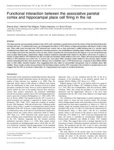
Figure 1 shows a detailed overview of our simulation system, which consists of three parts: our particle engine, a physics engine, responsible for particle-based objects, and a graphics renderer, which in our case uses Microsoft’s graphics API Direct3D 10.
4.1
Particle Engine
We have implemented the SPH method using CUDA and integrated in a simple particle engine. The most impor-
object surface particle velocity buffer
Position.X
Position.Y
Position.Z
PADDING
float
float
float
float
Velocity.X
Velocity.Y
Velocity.Z
PADDING
float
float
float
float
POSITION
60Hz
Physics engine
Particle engine object external force buffer
Density
object surface particle position buffer
fluid particle position buffer
VELOCITY
DENSITY
float Pressure object particle position buffer
60Hz
Direct3D renderer
PRESSURE
float Color
COLOR
float
Figure 2. Particle properties per particle video output
Figure 1. Overview of the simulation system. Our particle engine and the Direct3D renderer run in the same thread at 60Hz, whereas a physics engine, responsible for objects, runs in its own thread. Blocks that have two colors are double buffered buffers to prevent threading issues. The black dashed lines represent parts of the system that need to implemented. tant method in the engine is the update method, which performs the first four simulation steps described in section 6. The last step, which is the interaction algorithm is not implemented due to time constraints. The particle engine and the Direct3D renderer run in the same thread.
4.2 Direct3D Renderer We have also implemented a simple Direct3D renderer, that displays the fluid particles each frame. It can also display the density and pressure values per particle, the uniform grid, and the boundary particles. The most important method in the Direct3D renderer is the Render method, which first calls the update method of the particle engine, and then displays the fluid particles. Because the Direct3D renderer and the particle engine run in the same thread, the fluid particle position buffer is not double buffered, as there can be no threading issues.
4.3 Physics Engine For the physics calculations of objects, any physics engine can be used, as long as it supports applying user generated external forces, just like our SPH method supports an external force (see equation 2). The external forces will be provided by the interaction algorithm. For optimal performance, the physics engine should not run on the same GPU that our SPH implementation runs, but on a different GPU. In our case, we use the physics engine of the R platform. VICTAR⃝
5. DATA STRUCTURES In this section we will explain the data structures used in our implementation.
5.1 Particles
Particles consist of the following properties, which are stored in global memory: position, velocity, mass, radius, density, pressure, and the color property. These properties are all stored in their own array, which is called the structure of arrays instead of packing the properties into structures and placing them in one array (also called array of structures). The reason for this is that during the simulation steps, only a few properties are updated per step. For instance, in the second step of the simulation, the density of each particle is evaluated and the kernel responsible for this only needs the position and the density of each particle. The graphics hardware can fetch up to 128 bytes of memory per transfer, and if a structure with all properties would have to be fetched per particle, it would waste bandwidth, whereas fetching only data that is needed, we can achieve much higher efficiency. Another optimization we use to achieve maximum bandwidth is to pad the position and velocity arrays with one extra float, so that they are 16 bytes per element (four floats). This ensures that each element always starts at an aligned address, which enables the graphics hardware to fetch the elements efficiently and is called coalesced reading. The final optimization is the use of texture memory, where the texturing hardware on the GPU is used to fetch data. What makes using texture memory faster, is the fact that texturing hardware on the GPU makes use of a texture cache, where the data near the element that is sampled, is also stored in cache. Because of cache hits, global memory is less frequently used, therefore cutting down on bandwidth usage. Figure 2 shows the layout of the array elements that contain particle properties.
5.2 Uniform Grid To speed up finding neighbor particles, we use the simplest acceleration structure, which is the uniform grid. There are three reasons for choosing a uniform grid: • It is a simple structure and easy to implement. • The complexity of building a uniform grid is constant, because the number of particles and grid cells do not change during the simulation. • There is an upper bound to the amount of particles in a single grid cell (see figure 3). This limits the amount of particles that need to be taken into consideration when iterating over neighbor grid cells.
Figure 3. The upper bound of particles in a 3D uniform grid cell is eight, when each particle is placed on each corner of the grid cell. Pressure forces make sure that the particles do no go through each other. Figure 5. Uniform grid memory layout. the same data. These parameters are divided into two structures and are: • Uniform grid parameters. Contains the size of the grid, the dimensions of the grid (number of grid cells per axis) and the number of cells. • SPH parameters. Contains particle radius, particle mass, smoothing radius, gravity force, rest density, the stiffness constant, and the precalculated parts of the smoothing kernels that are constant.
Figure 4. A 2D uniform grid example with grid cell and particle ids.
The data in these structures are precalculated and updated once, at the beginning of the simulation. We have chosen to keep the particle mass, radius and smoothing radius constant, since we want to simulate a fluid where all particles are more or less equal.
6. The particles properties are sorted by particle id, and the goal of the uniform grid is to sort these properties by grid cell id. When we insert the particles into the uniform grid, we first calculate in which cell that particles is, then calculate a hash for that cell (which is simply the linear grid cell id). We then sort the position property array by cell id by using the CUDPP library [1], and also create two arrays called cellStart and cellEnd . These arrays contain indices per cell id, that point to start and end position in the sorted position array. Figure 4 shows an example of a 2D uniform grid with six particles and figure 5 shows the memory layout of the uniform grid. Finally we create another array that contains indices to the original particle position array, so that we can write evaluated density values as well as pressure and viscosity forces to the index of the unsorted particle position array. The reason we only sort the position property, is because it performs better since we do not have to sort all particle properties each step of the simulation.
5.3 Constants Several constant parameters are used for the simulation, and they are placed in so called constant memory, which is optimized for scattering where multiple threads read
SPH SIMULATION STEPS
The simulation is performed by repeating the following steps repeatedly: 1. Integrate particle properties. This means updating particle positions by applying pressure, viscosity, gravity and external forces to the particles. 2. Build a uniform grid for quick neighbor lookup. 3. Evaluate new density and pressure values. 4. Calculate the pressure and viscosity forces. 5. Apply the interaction algorithm These steps are explained in detail in the following sections and pseudo-code is given where deemed useful. Constant parameters in pseudo-code are written in uppercase. The given algorithms are applied to each fluid particle in parallel.
6.1 Integration of Particle Properties Integration of particle properties is the step where the calculated forces are used to calculate the acceleration of particles, and thereby updating their velocity and position. Our CUDA kernels, described in algorithms 1 and 2
in equation 2), calculate the acceleration of particles ( Dv Dt and write these values to an array. After the acceleration is calculated, the gravitational acceleration is added to it.
6.2 Building the Uniform Grid The uniform grid is rebuilt every time step of the simulation and consists of calculating the grid hash per particle and sorting the particle position array by cell index (as opposed to the array being sorted by particle index). This is done in the same way a uniform grid is built in the particles sample of the NVIDIA GPU Computing SDK [3].
6.3 Density and Pressure Evaluation Pseudo-code for evaluating the density and pressure values are given in algorithm 1. This algorithm solves both equation 4 and 5 together, since the result of equation 4 can directly be used to calculate equation 5. By calculating both equations at once, we do not have to iterate over the neighbor cells twice. First the position of the particle is retrieved (line 1) and its grid position is calculated by the helper method CalcGridPos (line 2). Then all neighbor cell are iterated (lines 4-6). The reason we iterate from -2 to 2 for each axis, is because each cell in the uniform grid is twice the radius of a particle (i.e. the size of a particle), and we have set the smoothing radius constant to four times the particle radius. So in order to find all particles within the smoothing radius, we need to check five grid cells in each axis, hence iterating from -2 to 2. Then the position and hash of each of the neighbor cells are calculated, using the helper method CalcGridHash (lines 7-8). The hash is then used to index the cellStart and cellEnd arrays (lines 9-11), which index the sorted position array (posArray). Then, for each of the particles in the neighbor grid cells, the distance squared is calculated (line 14) and if the particles lie in the smoothing radius squared, then densitySum is updated (lines 15-18). The index to the unsorted particle property arrays is retrieved (line 25) and finally the density and pressure are written to the density and pressure arrays (densArray resp. presArray). After the evaluation, the density and pressure arrays are copied into 512x512 textures, so that the next step can use the texturing hardware to retrieve the values outputted by this step. The size of the textures can be adjusted to the amount of particles that an implementation needs to support. Due to the size we have chosen, our version can support up to 262.144 particles.
6.4 Calculating Pressure and Viscosity Forces Algorithm 2 describes the process of calculating the pressure and viscosity forces (equations 6 and 7), thereby solving the − ρ1 ∇p (pressure force) and µ∇2 v (viscosity force) terms of equation 2. For the sake of brevity, we have replaced the neighbor cell iteration code with a for loop that loops over all particles in the neighbor cells, from firstParticle to lastParticle. Again, we calculate both equations 6 and 7 in the same algorithm so that the neighbor particles do not have to iterated twice. First the position and velocity are retrieved (pos resp. vel ), as well as the index to the unsorted property arrays (line 4). Then the texture index is calculated (line 5), since we use 2D textures and the index variable is an index to a 1D linear array. The texture index is used to retrieve the pressure (pres) for the current particle, by indexing the density and pressure textures (densTex resp.
Algorithm 1 Density and pressure evaluation Input: particleID, posArray, densArray, presArray, cellStartArray, cellEndArray, gridParticleID 1: pos ← float3 (posArray[particleID]) 2: gridPos ← CalcGridPos(position) 3: densitySum ← 0 4: for z = −2 → 2 do 5: for y = −2 → 2 do for x = −2 → 2 do 6: 7: neighborGridPos ← gridPos + int3 (x, y, z) 8: gridHash ← CalcGridHash(neighborGridPos) startIndex ← cellStartArray[gridHash] 9: 10: if startIndex ̸= empty then 11: endIndex ← cellEndArray[gridHash] 12: for i = startIndex → endIndex do 13: neighborPos ← float3 (posArray[i]) 14: distSqrd ← length(pos − neighborPos)2 if distSqrd ≤ SMOOTHINGRADIUS 2 15: then 16: h2 r2 ← SMOOTHINGRADIUS 2 − distSrdq 17: densitySum ← densitySum + h2 r2 3 18: end if 19: end for 20: end if 21: end for 22: end for 23: end for 24: density ← densitySum ∗ PARTICLEMASS + POLY6KERNEL 25: index ← gridParticleID[particleID] Output: presArray[index ] ← STIFFNESS ∗ (density − RESTDENSITY ) Output: densArray[index ] ← density
Algorithm 2 Calculating pressure and viscosity forces Input: particleID, posArray, velArray, presTex , densTex , gridParticleID, forceArray 1: pos ← float3 (posArray[particleID]) 2: vel ← float3 (velArray[particleID]) 3: gridPos ← CalcGridPos(position) 4: index ← gridParticleID[particleID] 5: texIndex ← int2 (index mod 512, index /512) 6: pres ← tex2D(presTex , texIndex .x, texIndex .y) 7: presSum ← float4 (0, 0, 0, 0) 8: viscSum ← float4 (0, 0, 0, 0) 9: for i = firstParticle → lastParticle do 10: neighborPos ← float3 (posArray[i]) 11: relPos ← pos − neighborPos 12: dist ← length(relPos) 13: if dist ≤ SMOOTHINGRADIUS then uID ← gridParticleID[i] 14: 15: uTexID ← int2 (uID mod 512, uID/512) nDens ← tex2D(densTex , uTexID.x, uTexID.y) 16: 17: nPres ← tex2D(presTex , uTexID.x, uTexID.y) 18: sr dist ← SMOOTHINGRADIUS − dist force ← ((pres + nPres)/(2 ∗ nDens)) ∗ (sr dist)3 19: 20: presSum ← presSum + (relPos/dist) viscSum ← viscSum + ((velArray[i] − 21: vel )/nDens) ∗ sr dist 22: end if 23: end for Output: forceArray[index ] ← (−presSum ∗ PRESSUREKERNEL + (DYNAMICVISCOSITY ∗ viscSum ∗VISCOSITYKERNEL))∗PARTICLEMASS
presTex ). Textures values are retrieved by sampling them using the tex2D method (lines 6, 16 and 17). The first parameter is the texture that needs to sampled and the next two parameters are the x and y position. Textures are always in the ranges 0.0 to 1.0, so the index retrieved on line 4 is divided by 512, because that is the size of the textures we use. We then iterate over all particles in the neighbor grid cells (line 9), and calculate the distance between the current and neighbor particle (line 10-12). If the distance is smaller than the smoothing radius, then we retrieve the density and pressure of the neighbor particle by indexing the respective textures (line 13-18) and calculate the pressure and viscosity forces, according to equations 6 and 7 (lines 19-21). Finally the forces are written to an array that contains the forces (forceArray).
7. INTERACTION ALGORITHM The interaction between fluid particles and object particles is a continuous process of repeating the following four steps:
7.2 Retrieving Object Surface Particles Usually the rate at which the physics are updated is higher than the display rate of the graphics, therefore the physics engine for the objects and the SPH implementation for fluids are going to run at different rates. Since the interaction algorithm affects both fluids and objects, this means that one engine (physics) has to wait for the other engine (SPH) to finish the calculations, in order to continue. One way to solve this problem is to use buffering, where one or more buffers are used for input and output, and the buffer that is updated can be used by the engine that needs it, while the other engine outputs to a different buffer. In the case of double buffering, two buffers are used and interchanged each time step of the simulation. Important is that a physics engine, responsible for the objects, only provides the surface particles of the objects, since these are the only particles that can be affected by collision detection. Two properties of surface particles need to be provided by a physics engine: the position and velocity. It also needs to provide a buffer to which the forces, that will be exerted on the surface particles, will be written by the SPH implementation.
1. Determine the surface particles of the fluid.
7.3
2. Retrieve the surface particles of the object(s). 3. Perform collision detection. 4. Calculate the forces that need to be applied to the particles of both the fluid and the object(s). These forces fall in the the external forces category that is used in the integration step of the SPH simulation. The first step and second step are obtaining the surface particles for the fluid and object(s), since these are the only particles that can have collision with each other, and therefore also has a lower complexity. The third and fourth steps are collision detection and calculating the forces that need to be applied to the fluid and object particles. These steps are explained in more detail in the following subsections.
7.1 Finding Surface Particles To determine which particles are on the surface of fluid, we use introduce a new property of a fluid particle, which is the color property. Normally, this property is used to calculate the surface tension of a fluid [13], but it can also be used to detect the position of the surface of the fluid, and find the normal vectors at the surface. This is important for realistic rendering of the fluid. The color property is a quantity that is either the value zero (not a surface particle) or one (is a surface particle). The following formula is used to calculate the smoothed average color (also called the color field) at particle i: Ci =
∑ mj Cj W (rj − ri ) ρj j
(11)
where Cj is the color property of particle j .
∑ mj Cj ∇W (rj − ri ) ρj j
Collision detection and force calculation between boundary and fluid particles was done by Harada et al. [6]. Their method uses two pieces of data to estimate the contribution of the wall particles to the density of the fluid particles. The first piece of data is the output of a distance function, where the distance from a particle to the wall is precalculated in each time step of the simulation, and stored it in a 3D texture. The second piece of data is a wall weight function, which is indexed by a texture coordinate calculated by the distance function. The output of the wall weight function is the density contribution of the wall, which is added to the particle in the first step of the SPH method. In section 3 we pointed out that Harada et al. made an improvement to the boundary condition [5], by using triangles to define objects instead of particles. We do not use this approach because of the use of triangles, since triangle-sphere collision is more complex than sphere-sphere collision. The latter is easily computed by taking the distance between two particles and subtracting both radii of the particles. If the result is smaller than zero, then there is collision. We have to note that this simple form of collision detection only works if the acceleration of particles is small enough that a collision can be detected at each time step. If the acceleration is too high, then between two time steps, a particle moves so fast that it passes other particles, so that a collision between them is not detected when it should be. For several ways to solve this problem, see section 8.
The gradient of the smoothed color field Ci , shows us where the surface is, and is given as ∇Ci =
Collision Detection
Detecting collisions can be solved by a couple of methods. Two of them are providing a density value based on the distance from a boundary, and performing basic spheresphere collision.
(12)
We tag particle i as a surface particle by setting the color property to one, when the magnitude of ∇Ci is greater than a certain value.
7.4 Force Calculation When a collision between two particles is detected, interparticle forces must be calculated. We use the discrete element method to calculate these forces [4], which are the repulsive force Frepulsive , modeled by a linear spring, a damping force Fdamping , modeled by a dashpot, and a shear force Fshear , which is proportional to the relative tangential velocity vij,t . The equations for each force be-
tween particle i and j are: Frepulsive = −kspring ((prad,i + prad,j ) − |rij |)
rij (13) |rij |
Fdamping = kdamping ∗ vij
(14)
Fshear = kshear ∗ vij,t
(15)
where vij,t is calculated as vij,t = vij − (vij ·
rij rij ) |rij | |rij |
(16)
In these equations, kspring is the spring coefficient, kdamping is the damping coefficient, kshear is the shear coefficient, prad,i and prad,j are the radius of particle i and j, rij is the relative distance vector and vij is the relative velocity vector. Since all particles are the same size in our case, we multiply the particle radius with two. Pseudo-code for a helper method that calculates these forces between particle i and j is given in algorithm 3. Algorithm 3 Calculating repulsive, damping and shear forces Input: posI , posJ , velI , velJ , forceArray 1: relPos ← posJ − posI 2: dist ← length(relPos) 3: diameter ← PARTICLERADIUS ∗ 2 4: force ← float3 (0, 0, 0) 5: if dist < diameter then 6: norm ← relPos/dist 7: relVel ← velJ − velI 8: relTanVel ← relVel − (dot(relVel , norm) ∗ norm) 9: force ← −SPRINGCOEFFICIENT ∗ (diameter − dist) ∗ norm 10: force ← force + DAMPINGCOEFFICIENT ∗ relVel 11: force ← force +SHEARCOEFFICIENT ∗relTanVel 12: end if Output: force
8. PITFALLS AND SOLUTIONS 8.1 Calibration of simulation parameters During the development of the SPH method in CUDA, we have had problems with fluid stability. SPH has many parameters that can be set (see 5.3), and they also require that the uniform grid parameters have to be set correctly. We found out that especially the rest density and stiffness coefficient are very sensitive, and have yet to find correct parameters for our implementation. Another issue we have is correctly calculating the repulsive forces when particles go outside the uniform grid, which we believe is also a calibration issue. This causes all fluid particles to gather at the bottom of the grid, filling all grid cells at the bottom with more than the maximum allowed of particles (see figure 3). As a result, a significant portion of computation time is spent iterating neighbor grid cells. We confirmed a significant decrease in computation time, when we limited the amount of iterations per neighbor grid cell to eight (see section 10 for results).
because the object particles are much larger than the fluid particles, and thus have bigger holes between them, or because the forces exerted on the object particles are great enough to enlarge the distance between object particles so that, again, the holes between them are large enough for the fluid particles to go through. To address the first problem, the size of the object particles can be made the same size as the fluid particles, or even smaller, so that the holes between them are smaller than the size of a fluid particle. This solution of course does not address the second problem, because objects can be made from a material that can be stretched easily, and therefore deform easily when a fluid exerts force on such an object. One solution to the second problem is to use a different and bigger radius, to create an influence sphere (see figure 6) when calculating the repulsive, damping and shear forces in equations 13, 14 and 15. We can then use the distance between fluid and object particles, to multiply the kspring term in equation 13 (see figure 7), with a distance function. This distance function can be calculated for a range of inputs, and the results can be written to constant memory as an array. Then this array can be used to estimate the result of the distance function, by using interpolation on the results in the array. As a fluid particle moves closer to an object particle, the influence of the repulsive force will become larger, keeping fluid particles at a distance. We have chosen an exponential distance function to multiply with the kspring term. As can be seen in figure 7, when a fluid particle comes very close to actually hitting the object particle, the additional increase of the repulsive force becomes so large, that it will simply bounce back. Another solution is a variation on the solution given above, and is dependant on the physics engine that is responsible for simulating the objects. If the physics engine is capable of detecting which particles are cut (for example in a physics engine that models springs between the particles), then the influence on the damping coefficient can be disabled, because the artery is damaged. The difference between these two solutions is that in the first solution, the state of an object (whether is cut or not) is implicitly described by the way the damping coefficient is influenced, which can lead to a lot a less stable simulations, because the influence has to be tweaked per material of the object. The second solution does not suffer from this flaw. Both solutions will have to perform sphere-sphere collision detection per radius that is used, which increases complexity, but since the collision detection complexity is very low, we do not expect this to be the speed limiting factor in the simulation.
8.3 Collision Detection In section 7.3 we stated that a simple sphere-sphere collision detection, does not work properly if particle acceleration is too high. Two ways to solve this problem are mentioned in this section.
8.2 Fluids passing through objects
Continuous collision detection is a method that, given two points in time, can determine if there is a collision between objects, and when. One algorithm to perform continuous collision detection in parallel on GPUs has been developed by Tang et al. [18]. Although their algorithm can not be directly used to detect collision between spheres, it does give us an indication that continuous collision detection could be fast enough to achieve interactive rates.
In section 2.2 we described a scenario where fluid particles can go through the particles of an object. This can be
Another approach is to limit the amount of acceleration of particles. This can be done on a per-particle basis,
but the simplest way is to define a new constant, which is the maximum allowed amount of acceleration for all particles in the simulation. The downside to this approach is that this constant possibly has changed per simulation, depending on other parameters of SPH and used objects.
9.
TEST CASE
To test the interaction algorithm, a virtual artery made of particles will be filled with the SPH fluid particles, varying the amount of particles for both the artery and the fluid for each test. When a test is run, determining if the interaction algorithm is stable is necessary (i.e. fluids do not pass through the artery, unless it is torn open). One way to test the stability is to completely fill the artery with fluid particles, and squeeze one side of the artery, which should push all fluid particles to the other side of the artery, without flowing outside of it. Figure 6. Front and side view of an interaction example, using a different radius to calculate equations 13, 14 and 15. An object particle has a size (grey sphere), but the influence sphere (dashed sphere) is used in the interaction algorithm, when a fluid particle (orange) collides with it.
Also, the influence of the size of the influence sphere (see section 8.2) on computation time, should be determined. Increasing the influence sphere, means that a fluid particle can collide with multiple object particles, and for each of them, the repulsive, damping and shear forces have to calculated. This increases the computation time.
10.
RESULTS AND EXPECTATIONS
We have implemented the SPH method in CUDA version 4.0. In our application, a set amount of fluid particles are dropped in a box, the same size as the uniform grid. We ran two different tests with a different amount of particles per test. The difference between the two tests is that in the second test, we limited the amount of neighbor particles per grid cell to eight, to get an indication of how fast our implementation would be, if we had correct simulation and SPH parameters. The result of these tests can be found in tables 1 and 2. R Our test setup was a computer with an 3.4GHz Intel⃝ R Core⃝ i7-2600K CPU, a mainboard with an Intel P67 chipset, 8GB of ram, and an NVIDIA GeForce GTX 480 graphics card with 480 CUDA cores and 1.536MiB of memory.
Looking at our results, we can see the importance of correctly calibrated simulation parameters. When we limit the amount of neighbor particles to eight (see figure 3), we see that the simulation runs significantly faster, and that even simulating fluids with 266.144 particles in realtime, is possible.
kspring
distance function distance
Figure 7. Example of a distance function, which is multiplied with the kspring term in equation 13, depending on the distance between the fluid particle (orange) and the influence sphere (dashed sphere).
Though we did not implement the interaction algorithm, we can make a reasonable prediction about the speed of a potential implementation. The particles sample in the NVIDIA GPU Computing SDK [3], is a particle simulation, where particle collisions are also performed by the discrete element method method [4]. It can simulate 65,536 colliding particles at about 460 frames per second on a R GeForce⃝ GTX 480 [3]. Though our algorithm is of higher complexity because of the adjustment of the damping force, which is not present in the particles sample, their sample does show us that the collision detection and force calculation itself, can be run at a multitude of the speed we would like to achieve. Based on the results of our implementation and the particles sample, we expect that a complete implementation, running on the GeForce GTX 480, can simulate up to 60.000 particles, while maintaining interactive rates of at least 60Hz. We estimate this amount of particles, because we showed that a correctly calibrated SPH implementation, simulating 65.536 particles, takes 11.4 milliseconds
Table 1. First test: no limit to the amount of neighbor particles per grid cell. Computation times are including rendering time. Number of particles Time in milliseconds 4.096 3.2 10.000 9.1 16.386 14.7 65.536 166.7 100.000 330.3 266.144 998.0 Table 2. Second test: eight particles per neighbor grid cell. Computation times are including rendering time. Number of particles Time in milliseconds 4.096 1.5 10.000 2.3 16.386 3.5 65.536 11.4 100.000 16.9 266.144 41.7 to compute all SPH forces, and the particles sample takes around 2.2 milliseconds. This adds up to a theoretical 13.6 milliseconds, which is 3 milliseconds less than our goal of 16.6 milliseconds for 60Hz. Furthermore, we expect that the interaction algorithm is stable. Since the algorithm only requires an array that contains the position and velocity for each surface particle of an object, we also expect it to be flexible and relatively easy to integrate it within existing physics engines, be written as a library that is easy to use. This can then be used for medical surgery applications, as well as any other application that needs interaction between SPH fluids and dynamic, particle-based objects.
11. FUTURE WORK AND CONCLUSION The first step is to correctly calibrate the SPH parameters, since they are very important to create a stable simulation. We have also shown that, when particles do not gather together in a heap, and the upper limit of particles in a grid cell is respected, that the simulation speed increases significantly. The next step is implement our interaction algorithm. It can then be tested as described in section 9 to determine the stability of the implementation and to measure the speed of the interaction algorithm. We have also shown that there is a good possibility that up to 60.000 particles in total can be simulated at interactive rates of 60Hz, based on our results and the results of NVIDIA in their particles sample [3].
12. ACKNOWLEDGEMENTS The author would like to thank M.I.A. Stoelinga, MSc, PhD, and M. Weber, MSc, PhD, for their valuable guidance and support. The author would also like to thank E.E. Kunst, MSc, PhD, and A.J.B. Sanders, BSc, at Vrest Medical for allowing the integration of the SPH implemenR platform, and providing the tation within the VICTAR⃝ much needed and necessary resources for this research.
13. REFERENCES [1] cudpp. cudpp - cuda data parallel primitives library, 5 2011.
[2] R. A. Dalrymple. Levee breaching with gpu-sphysics code. In 4th SPHERIC Int. Workshop, pages 352–355, 2009. [3] S. Green. Particle Simulation using CUDA. 2010. [4] T. Harada. Real-time rigid body simulation on gpus. In H. Nguyen, editor, GPU Gems 3, chapter 29. Addison Wesley Professional, Aug. 2007. [5] T. Harada, S. Koshizuka, and Y. Kawaguchi. Improvement in the boundary conditions of smoothed particle hydrodynamics. Computer Graphics & Geometry, 9(3):2–15, Winter 2007. [6] T. Harada, S. Koshizuka, and Y. Kawaguchi. Smoothed particle hydrodynamics on gpus. pages 63–70, 2007. [7] T. Harada, Y. Suzuki, S. Koshizuka, T. Arakawa, and S. Shoji. Simulation of droplet generation in micro flow using mps method. JSME International Journal Series B Fluids and Thermal Engineering, 49(3):731–736, 2006. [8] S. Koshizuka and Y. Oka. Moving-particle semi-implicit method for fragmentation of incompressible flow. Nuclear Science and ˝ Engineering, 123:421U434, 1996. [9] L. B. Lucy. A numerical approach to the testing of the fission hypothesis. Astronomical Journal, 82:1013–1024, December 1977. [10] M. M¨ uller, D. Charypar, and M. Gross. Particle-based fluid simulation for interactive applications. In Proceedings of the 2003 ACM SIGGRAPH/Eurographics symposium on Computer animation, pages 154–159, 2003. [11] M. M¨ uller, S. Schirm, and M. Teschner. Interactive blood simulation for virtual surgery based on smoothed particle hydrodynamics. Technol. Health Care, 12(1):25–31, 2004. [12] J. J. Monaghan. Smoothed particle hydrodynamics. Annual Review of Astronomy and Astrophysics, 30:543–574, 1992. [13] J. P. Morris. Simulating surface tension with smoothed particle hydrodynamics. International Journal of Numerical Methods in Fluids, 33:333–353, 2000. [14] NVIDIA. CUDA C Best Practices Guide 3.2. 2010. [15] S. Premoze, T. Tasdizen, J. Bigler, A. Lefohn, and R. T. Whitaker. Particle-based simulation of fluids, 2003. [16] K. Shibata, S. Koshizuka, Y. Oka, and K. Tanizawa. A three-dimensional numerical analysis code for shipping water on deck using a particle method. ASME Conference Proceedings, 2004(46911):959–964, 2004. [17] G. Stinson, J. Bailin, H. Couchman, J. Wadsley, S. Shen, C. Brook, and T. Quinn. Cosmological galaxy formation simulations using sph. ArXiv eprints, 000(April):16, 2010. [18] M. Tang, D. Manocha, J. Lin, and R. Tong. Collision-streams: Fast GPU-based collision detection for deformable models. In I3D ’11: Proceedings of the 2011 ACM SIGGRAPH symposium on Interactive 3D Graphics and Games, pages 63–70, 2011.