interactive computer methods for morphometric and ...

INTERACTIVE COMPUTER METHODS FOR MORPHOMETRIC AND KINEMATIC MEASUREMENT OF IMAGES OF THE SPINE

A thesis presented for the degree of Doctor of Philosophy at the University of Aberdeen

Steven Brian Harvey BEng (Wollongong) MEng (Wollongong)

1999

SUMMARY The aim of this project was to develop robust interactive computer methods for measuring the shape and movement of the lumbar spine vertebrae from lateral radiographs of the spine. In order to achieve this aim, two software packages were written - the Aberdeen Vertebral Morphometry System (AVMS) and the Aberdeen Spinal Videofluoroscopy System (ASVS).

AVMS was designed to analyse static images from dual energy x-ray absorptiometry (DXA) imaging densitometers. Comparative precision tests of the ability of AVMS software and Lunar EXPERT-XL software to measure vertebral height were undertaken using four vertebrae from the same lateral spine image. The image chosen was obtained by dual energy xray absorptiometry (DXA) from the same subject (male, 67 years). Two of the vertebrae in this image were abnormal and two were normal.

The

AVMS software had significantly higher (p 75% slippage. In retrolisthesis, a lumbar vertebra is rearwardly displaced with respect to the vertebra beneath it.

Osteophytes are bony outgrowths (spurs) usually occurring at the margins of joint surfaces.

In the vertebral column they form near the vertebral

endplates and reduce the space available in the spinal canal (White & Panjabi, 1990). Osteophytes are believed to be a physiological response to compressive loads (Macnab, 1971).

This has been confirmed in

epidemiologic studies carried out by Nathan (1962) that correlate the presence of osteophytes with a history of heavy labour.

2.3.2 Quantifying structural abnormalities Genant et al. (1993) have developed a semi-quantitative approach to vertebral fracture assessment, whereby vertebrae T4-L4 are graded on visual inspection of radiographs without direct measurement. The advantage of their semiquantitative methods over other quantitative approaches using digitised vertebral dimensions is that fractures such as

16

CHAPTER 2 - THE SPINE AND ITS MOVEMENTS

those of the end plates are readily distinguished, thereby indicating a vertebral fracture. Genant et al. argue that quantitative approaches that use vertebral height measurements digitised from radiographs are subject to errors due to parallax distortion and varying radiographic quality. However they fail to address the fact that recent advances in dual-energy xray absorptiometry (DXA) technology have meant that second generation scanners are now able to produce digital spine images of sufficient resolution to be used in the assessment of vertebral body shape (Harvey et al., 1998a).

Such images are minimally affected by parallax distortion

(Blake et al., 1997).

Vertebral morphometry is the quantification of vertebral body shape from measurements performed on lateral radiographs of the lumbar and thoracic spine, under carefully standardised conditions (Blake et al., 1997). This technique requires the placing of reference points on radiographs to represent the shape of the vertebral body. There are many different marker placement schemes in current usage, each using a different number of points to represent the shape of the vertebral body. Figure 2.9 depicts some of the better known schemes.

Figure 2.9. Different vertebral morphometry marker placement schemes. a) Jensen & Tougaard (1981) b) Smith-Bindman et al. (1991) c) Mayo Clinic (Nelson et al. 1990) d) Genant et al. (1993) e) McCloskey et al. (1993) f) Frobin et al. (1997).

17


Parameters measured using these marker points are the anterior height (ha), mid-vertebral height (hm) and posterior height (hp) as shown in Figure 2.10.

Figure 2.10. Heights measured from markers placed on lateral radiographs of the vertebral body - anterior height (ha), mid-vertebral height (hm) and posterior height (hp).

Three types of fractures may be detected using ratios of these vertebral heights: wedge (decreased ratio of ha/hp), biconcavity (decreased ratio of hm/hp) and crush (decreased ratio of hpi/hpi+1 or hpi/hpi-1) where i refers to the current vertebra, i+1 the adjacent vertebra above and i-1 the adjacent vertebra below.

Vertebral height measurements differ widely between patients, depending on stature. It is, therefore, important that some means of scaling these measurements be adopted. Minne et al. (1988) have scaled by reference to T4 (which, unfortunately, may itself be fractured), while Eastell et al. (1991) have made use of the implicit scaling present in the ratios of the vertebral heights. As well as scaling for stature, Eastell’s method also corrects for any variation in the magnification of the radiograph.

In the Eastell

classification, a vertebra is considered fractured if any one of the three height ratios is more than 3 standard deviations (SD) below the normal mean for that vertebra. Black et al. (1991) used normative values of the wedge, biconcavity and crush ratios developed by Eastell et al. (1991) to derive mean and population SD values for each vertebral level. The 3SD criteria was used to detect vertebral fractures. Melton et al. (1993) followed a similar technique but with a smaller sample size. 18


In Chapter 4 of this thesis an alternative method for measuring vertebral heights is discussed.

The method, termed the Aberdeen Vertebral

Morphometry System (AVMS), uses 11 markers to define the shape of a vertebral body on a digital radiograph. Apart from the anterior, middle and posterior heights, additional information such as the presence of osteophytes can be extracted from the radiograph using AVMS.

2.4

Dynamic aspects of the spine

2.4.1 Normal motion This thesis is partially concerned with the kinematics of the human spine, and this section concentrates on its normal movements. Although there have been many studies of normal motion of the spine (e.g., Frymoyer et al., 1979), still very little is known about it.

Translation or rotation of the spine can occur in any of the three fundamental anatomical planes shown in Figure 2.2.

The four normal

physiological motions of the spine are termed flexion (forward sagittal bending), extension (backward sagittal bending), lateral bending (in the coronal plane) and axial rotation (in the transverse plane). Figure 2.11 depicts these motions.

19


Figure 2.11. The four physiological motions of the spine. a) Flexion. b) Extension. c) Lateral bending. d) Axial rotation (adapted from White & Panjabi, 1990).

These four normal physiological motions of the are inherently connected one motion is always accompanied by another (White & Panjabi, 1990). This effect, termed coupling, may be attributed to vertebral geometry (zygapophyseal joints), connective tissues, natural curvature of the spine and directions of muscle actions. The main motion may be defined as that motion which most closely corresponds to the intention of the person who is moving, while the accompanying motions are called coupled motions. In the particular case of flexion-extension of the spine, which forms the focus of the kinematic part of present study, flexion-extension is the main motion, and the individual anterior/superior vertebral translations and rotations are the coupled motions. As the present study is principally concerned with the lumbar spine, the normal movements exhibited by the lumbar spine will now be described.

During flexion, the entire lumbar spine leans forwards on the sacrum, by the straightening of the lumbar lordosis (White & Panjabi, 1990). Maximum flexion is achieved when the lumbar spine attains a straight alignment, whereby each vertebrae rotates from the backward tilted

20


position (upright lordosis) to a position where the superior and inferior surfaces of adjacent vertebrae are parallel. The main motion of vertebral anterior sagittal rotation is accompanied by a forward translation. This forward translation is restricted by the zygapophyseal joints, and the anterior rotation resisted by the ligaments of the intervertebral joints (Bogduk & Twomey, 1991). Flexion itself is a two part movement involving both the spine and the pelvis in the sagittal plane. The first 60° of forward bending may be attributed to intervertebral motion while an additional 25° is due to hip motion (White & Panjabi, 1990).

Intervertebral extension movements are the opposite to those occurring in flexion. That is, the lumbar vertebrae undergo posterior sagittal rotation accompanied by a small posterior translation. Movement is limited by the contact of adjacent vertebrae. Pearcy (1985) reported that the total normal range of motion of the spine is from 55-83° in flexion-extension.

Axial rotation of the lumbar spine involves twisting of the intervertebral discs and is limited by the contact of the zygapophyseal joints. It has been calculated by Hickey & Hukins (1980) that the maximum range of rotation of an intervertebral disc without damage is approximately 3°. This is based on the observation that collagen fibres are limited to 4% strain without damage.

The zygapophyseal joints and posterior ligaments protect the

fibres of the annulus from excessive tension, and provide a buffer in the first 3° of rotation. Pearcy (1985) reported a normal range of axial rotation of 415° for the whole spine.

Lateral bending of the lumbar spine involves a combination of bending and rotating movements of intervertebral joints. Pearcy (1985) found the range of lateral bending in normal individuals to be 15-48°. Very little is known about the coupling characteristics of lateral bending.

21


Axial compression occurs as a result of the weight bearing function of the spine in the upright posture and from muscle action. The annulus fibrosus and nucleus pulposus bear the load and transmit it to the vertebral endplates.

The weakest components of the intervertebral disc are the

vertebral endplates when subjected to axial compression (Perey, 1957).

Axial distraction (tension) is a load that the lumbar spine is not normally subjected to, given that humans spend most of their time in the upright posture, bearing compressive loads. As a result, very little is known about the behaviour of the lumbar vertebrae when subjected to axial tension. However, it has been shown (Cyron & Hutton, 1981) that the zygapophyseal joints are able to bear up to twice the body weight in tension if necessary.

The concept of the functional spinal unit (FSU), or ‘motion segment’, will now be introduced. This is the smallest segment of the spine able to exhibit similar motion characteristics to the spine as a whole (White & Panjabi, 1990). It consists of two adjacent vertebrae and their connecting tissues, the lower vertebra being the reference with displacements measured from the upper vertebra. The FSU concept is important when examining the motion of the spine because it isolates relative motion at a particular level and enables comparisons between levels to be made.

2.4.2 Quantifying abnormalities One of the main functions of the joints is to permit motion, and pain may impair this function, the pain frequently being due to joint disorders (Stokes et al., 1987). The spine, being a complex system of joints, is subject to this impairment - the prevalence of low back pain has been cited by many authors as a cause of abnormal spinal motion (Pearcy et al., 1985). Conversely, other investigations have theorised that excess mobility of the spine is a pathological sign in patients with low back pain (Harris & MacNab, 1954, Mensor & Duvall, 1959).

22

Unfortunately, the term


‘instability’ has been coined as an all-encompassing title for abnormal flexion-extension spinal motion (Gertzbein et al., 1985). The more refined definition of instability given by White & Panjabi (1990) includes other factors as well. So there appears to be not only confusion as to the cause of abnormal spine motion, but in its description as well. What is clear is that there is no obvious correlation between specific motion patterns and the pain or deformity that they are supposedly caused by. In the kinematic part of this work the concept of instability will not be debated; rather the physiological sign of abnormal motion as an indicator of degeneration will be investigated.

In the United States alone over 70,000 lumbar fusion procedures are carried out annually in response to severe low back pain (Esses et al., 1996). Fusion may change the motion signature of contiguous lumbar intervertebral levels, but there is very little data available from controlled studies to confirm this (Esses et al., 1996). In this work, abnormal motion in flexionextension is investigated, in particular the motion of individual vertebrae. This is best done at the FSU level whereby the motion of one vertebra can be seen relative to another. Although abnormal motion may be exhibited by the spine as a whole, this motion can be described as the sum of the movements at the individual FSUs. The abnormality may be greatest at one particular level.

Pioneering work by Knutsson (1944) revealed the possibility that vertebral translation in the sagittal plane was an early indication of disc degeneration. Another early study by Tanz (1953) found a large variation in intervertebral angles among normal discs while Begg & Falconer (1949) found increased and decreased angular mobility at different stages of degeneration. This tends to nullify the reliability of intervertebral angular measurement.

23


In order to clarify this situation, instantaneous centres of rotation (ICRs) measured from radiographs have been used for many years to quantify abnormal intervertebral motion (Pearcy & Bogduk, 1988). Unfortunately this technique is subject to high levels of inaccuracy, particularly when small angles of rotation are used and when near-pure translation is found (Panjabi et al., 1992).

However, Seligman et al. (1984) did show that

degenerate spinal FSUs in vitro displayed more erratic ICR loci (‘centrodes’) than normal FSUs.

Gertzbein et al. (1986) were interested in observing the quality, rather than the quantity, of motion using the Moire Fringe technique. The loci of the ICRs were determined for several points in flexion-extension, the clusters of points termed centrodes, and their characteristic patterns studied. Additional studies characterised centrode patterns in spines with varying degrees of disc degeneration. In those spines with degenerate discs, the centrode pattern increased .in length and was at a different location. However, Penning et al. (1984) previously found that the expected 'abnormal’ centrode patterns in subjects showing signs of disc degeneration were not present.

In many studies, for example Stokes et al. (1987), it has been concluded that flexion-extension radiographs are not useful in the detection of abnormal lumbar intersegmental motion. Plain radiographs show the position of the spine in selected postures only and dynamic abnormalities would only be detected radiographically if they were manifested at the static end points of the motion. Penning & Blickman (1980), however, did use plain flexionextension radiographs to examine the spinal motion of patients having spondylolisthesis, and found that they did exhibit increased magnitude of motion compared to asymptomatic subjects.

The inherent difficulties in recording intervertebral motion could be overcome using cineradiogaphy, but at the expense of larger radiation

24


exposure. The degree to which the measurement of segmental motion can be used in the diagnosis of lumbar spinal disorders is unclear, due mainly to the technical and ethical difficulties of recording and measuring the motion. These technical problems may be part of the reason for disappointing results from motion studies of the spine.

Videofluoroscopy, however,

promises to overcome many of the technical and ethical difficulties associated with quantifying dynamic abnormalities.

Details of this

modality are given in the following chapter. Chapters 5, 6 and 7 of this thesis describe an application of videofluoroscopy to the motion of the spine.

25

CHAPTER 3 - IMAGING MODALITIES

CHAPTER 3 - IMAGING MODALTIES 3.1

Introduction

Medical imaging is concerned with the generation of useful images of the human body. The interpretation of medical images requires the inference of three-dimensional anatomical details from two-dimensional data. Due to the high incidence of low back pain (National Back Pain Association, 1991) and the inaccessibility of the spine to non-invasive clinical examination, heavy reliance has been placed on medical imaging techniques for spinal investigations.

In particular, plain (static) radiography has been the

modality of choice of practitioners who are seeking information about spinal structure and function (Thorkeldsen & Breen, 1994) since it is already an accepted medical imaging tool. A survey by Park (1980) estimated that 4% of the workload in British radiology departments was related to lumbar spine examinations. Most of the requests were to examine patients with non-specific low back pain.

While exhibiting excellent resolution, this

modality does have some inherent weaknesses such as geometric distortion and high radiation dosage to the patient (Wall & Hart, 1997).

Dual Energy X-ray Absorptiometry (DXA) imaging has been refined to the point where it is now possible to obtain near-radiographic quality images (Ergun et al., 1995) of the vertebral column at a fraction of the radiation dose of equivalent plain x-rays (Steel et al., 1998).

Static magnetic

resonance imaging (MRI) is also used to evaluate the soft tissue regions of the spine (Miller, 1996) and has the advantage of not exposing the patient to ionising radiation (Smith, 1982) while still providing excellent soft tissue detail (Weng & Haynes, 1996).

There now exists an increased awareness among practitioners of the importance of treating the spine as a dynamic system rather than solely a static structure (McGregor et al., 1997). This has led to the development of dynamic radiographic imaging techniques that enable a sequence of images

26


of the moving spine to be recorded for subsequent analysis. In all cases, these techniques are an adaptation of an existing imaging modality, for example cineradiography (Jones, 1962). Videofluoroscopy, commonly used for imaging the gastro-intestinal tract, has also been successfully applied to the imaging of the moving spine (Kanayama et al., 1996; Cholewicki & McGill, 1992).

While producing poorer quality images than plain

radiography, the benefits of videofluoroscopy include lower radiation dose (Breen et al., 1993) and ease of directly storing images in digital format. Development continues into the use of kinematic MRI for imaging moving regions of the body. Common areas of study include planar joints such as the knee (Brossmann et al., 1993), although the shoulder is also an area of application (Bonutti et al., 1993). The potential exists for kinematic MRI to be used to image the moving spine, although this has not yet been achieved.

Research work carried out in this thesis has made use of both static (DXA, MRI) and dynamic (videofluoroscopy) imaging modalities.

This chapter

serves to introduce these modalities and covers brief technical details and applications relevant to the spine. Also discussed are plain radiography and kinematic MRI since they are very closely related to the other modalities for spinal imaging.

A brief introduction to radiation dosimetry and image

quality now follows.

3.2

Radiation dosimetry and image quality

The following information on radiation dosimetry and image quality is based on Dowsett et al., (1998), and the reader is directed to this text for further details on the physics of radiology. The traditional unit of x-ray exposure was originally termed the roentgen, R. Nowadays, measurement of x-ray exposure is by means of the internationally accepted unit of ionising radiation coulomb per kilogram, C/kg. The two units are related by 1 C/kg = 3876 R. Exposure is a property of the x-ray beam and therefore not a true indicator of energy absorbed by the irradiated material, which may have an

27


atomic number quite different to that of air. Therefore an additional term, the absorbed dose is also used.

Absorbed dose was traditionally measured in rads (roentgen absorbed dose) but now is expressed as J/kg or gray (Gy). The two units are related by 1 Gy = 100 rads. The absorbed dose is conventionally averaged over a tissue or organ and statistically weighted according to the radiation type and radiosensitivity of the organs being irradiated, resulting in the effective dose (ED). This is measured in sieverts (Sv). Effective dose expresses the overall measure of health detriment associated with each irradiated tissue or organ as a whole body dose. Hart et al. (1994) specify equation 3.1 for converting absorbed dose (in the form of dose-area product) to effective dose for the lateral lumbar spine: ED = DAP × 0.00108

(3.1)

where ED is effective dose in mSv and DAP is dose-area product in cGy.cm2. Table 3.1 shows the effective dose values from a variety of radiological examinations and other sources.

The image on an x-ray film is produced by light emitted from scintillation screens placed on either side of it. The same principle applies to newer techniques such as image intensifiers and computed tomography where intensifying screens or electronic detectors are used in place of conventional silver emulsion film. The resulting image may be considered as a grey scale revealing the background intensity of scattered x-rays (noise) overlaid with the accumulated transmission of x-rays by the tissues and air gap through which they have passed (attenuation).

The degradation of image spatial resolution is commonly termed image ‘unsharpness’, representing the combined effects of geometrical, movement and radiographic unsharpness.

Geometric unsharpness is influenced by

28


distances between x-ray tube, patient and image plane as well as focal spot size.

Movement unsharpness is caused by the movement of the patient

and/or organ. Radiographic unsharpness causes image blurring due to poor film/screen contact and passage of light within the phosphor material which generates the film or fluoroscopic image.

Table 3.1 Effective dose values to standard adult patients for radiological examinations and other sources 3

EXAMINATION

ED (mSv)

REFERENCE

Minimum lethal dose

3500

Heaton (1995)

Minimum dose for serious radiation sickness

1500

Heaton (1995)

NRPB Annual radiation limit - workers

50

Shrimpton et al. (1986)

CT scan pelvis

10

Wall & Hart (1997)

CT scan chest

8.0

Wall & Hart (1997)

Barium enema examination

7.69


Spinal videofluoroscopy (10 s)

6.3

Breen et al., (1993)

Nuclear medicine bone investigation

5.68

Dowsett et al. (1998)

NRPB Annual radiation limit - public

5.0


Natural annual background radiation

4.0


Barium meal examination

3.83


Typical annual dose - airline pilots

3.0

Heaton (1995)

Mammographic examination

2.20

Heaton (1995)

Lumbar spine examination

2.15


CT scan head

2.0

Wall & Hart (1997)

Single lumbar spine radiograph (AP1)

0.90


Single lumbar spine radiograph (LAT2)

0.53


Single thoracic spine radiograph (AP)

0.40

Wall & Hart (1997)

Single thoracic spine radiograph (LAT)

0.30

Wall & Hart (1997)

Spinal videofluoroscopy (13 s)

0.15

Table 6.2

DXA LAT spine scan (Lunar EXPERT-XL imaging densitometer - morphometry mode)

0.07

Steel et al. (1998)

DXA AP spine scan (Lunar EXPERT-XL imaging densitometer - fast mode)

0.06

Steel et al. (1998)

Transatlantic flight

0.04

Kalender (1992)

Single skull radiograph (AP)

0.03

Wall & Hart (1997)

Single chest radiograph (PA)

0.02

Dowsett et al. (1998)

Equivalent cancer risk from one cigarette

0.02

Heaton (1995)

1

Anterior-posterior. Lateral. 3 Effective dose. 2

29


Image quality is degraded by noise which is seen as fluctuations in image density. These fluctuations reduce the level of low contrast detectability of the system and sharpness of the image.

It is also influenced by the

graininess of the film, phosphor sensitivity and quantity of x-ray photons. Image noise becomes more obvious if the photon number is small. Image intensifier systems use far fewer photons for image formation than film systems and so are more susceptible to image noise.

3.3

Static imaging of the spine

3.3.1 Plain radiography The term ‘plain radiography’ refers to the use of a single x-ray film placed adjacent to the patient to capture a static image of the resulting attenuation pattern.

While exhibiting excellent resolution, this modality does have

some inherent weaknesses such as geometric distortion (Steiger et al., 1994) and high radiation dosage to the patient (Wall & Hart, 1997). Quantitative measurements are usually taken from plain radiographs by means of a viewing box, pencil, ruler, and digitising tablet (Dvorak et al., 1991, Panjabi et al., 1992). Stokes (1990) describes the application of plain radiographic techniques to the spine and the reader is directed to this publication for additional information.

Plain radiography is able to show the form and alignment of the vertebral column including the presence of fractures and congenital defects. For instance, spinal curvature may be evaluated by measuring the distance between the inclination of two specified vertebrae (Polly et al., 1996). Vertebral shape may also be measured using plain radiography in order to identify the presence of vertebral fractures (Section 2.3.2). Lateral spine images are particularly useful for visual assessment of abnormalities such as intervertebral disk expansion and osteophytes. Leiviska et al. (1985) found that measurements taken from plain films were a reasonable

30


alternative to those from CT scans.

Measurements

of

intervertebral

motion

may

be

made

by

the

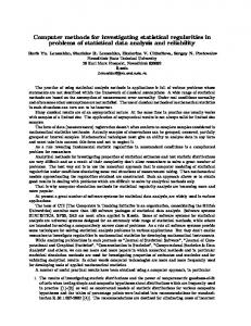
superimposition of two vertebrae on two plain radiographic exposures (Figure 3.1).

Motion is calculated as the relative difference in two

successive angles between the radiograph borders for the particular superposition level. Typically flexion and extension films are used (Keessen et al., 1984, Frobin et al., 1996), although lateral bending may be evaluated using anterior-posterior (AP) films (Dvorak et al., 1991).

Figure 3.1 Measurement of intervertebral motion. Lateral radiographs are taken with the subject extended and then fully flexed. The extension radiograph is taped to a viewing box, the flexion radiograph overlaid and the images of the selected vertebra superimposed. The angle between the borders of the radiographs represents the flexion angle. This process is repeated for the adjacent vertebra. The difference in the flexion angles between these two successive superpositions represents the intervertebral motion. Adapted from Stokes et al., (1987).

However, taking differences in this way is known to produce large measurement errors (Stokes, 1990) since any errors are accumulated throughout the vertebral column.

This is particularly important in the

measurement of small amounts of angular and linear motion. In addition, any

out-of-plane

motion

will

introduce

31

further

errors

into

the


measurements. Fortunately, flexion and extension generally occur without any appreciable out-of-plane motion (lateral bending or axial rotation) (Pearcy, 1985) and it has been shown that the superposition technique for measuring intervertebral flexion and extension on lateral radiographs correlates well with three-dimensional studies (Portek et al., 1983). If the measurement of motion in three dimensions is required, however, stereo radiographic techniques need to be used (Pearcy 1985). These methods have been used in the study of the mobility of a degenerate vertebral level and its adjacent segment before and after lumbar fusion (Axelsson et al., 1997). Accurate and comparable measurements from two-dimensional (plain) radiographic techniques are only possible if the positioning of the subject and x-ray equipment is carefully controlled.

Plain radiography, however, exposes the patient to a high radiation dose (Wall & Hart, 1997) and is subject to wide variation in acquisition and interpretation.

A minimum of two plain radiographic exposures are

required to image the entire thoracolumbar spine (Blake et al., 1997) due to geometric distortion effects and attenuation differences (Steiger et al., 1994), which in turn vary from institution to institution.

For computer-aided

analysis the films must first be digitised, a step which further reduces the integrity of the original data. Some of these problems have been addressed by the development of DXA imaging of the spine, which will now be discussed.

3.3.2 Dual energy x-ray absorptiometry (DXA) imaging Dual energy x-ray absorptiometry (DXA) has become the single most widely used technique for performing bone densitometry studies since its introduction a decade ago (Blake & Fogelman, 1997).

One of the most

important applications of DXA has been its widespread use in the diagnosis of osteoporosis and assessment of vertebral fractures due to the well established link between bone mineral density (BMD) and fracture risk

32


(Black et al., 1992). For further reading on the technical principles of dual energy x-ray absorptiometry the reader is directed to the work of Blake & Fogelman (1997).

Recent advances in DXA technology have meant that second generation scanners are now able to produce digital spine images of sufficient resolution to be used in the assessment of vertebral body shape (Harvey et al., 1998a).

This process, termed vertebral morphometry, has been

discussed in Section 2.3.2. There are two major advantages in using DXA images for vertebral morphometry over plain radiographs. The first of these is lower patient radiation dosage. An effective dose of 0.071 mSv has been reported for a typical lateral spine morphometry scan (Steel et al., 1998), representing a considerable dosage reduction over conventional plain film radiographs (Table 3.1). Secondly, DXA scanners are now able to digitally image the entire T4-L4 range in a single pass, thereby eliminating the need for two separate radiographic exposures and the associated geometric distortion due to a cone-beam x-ray source (Blake et al., 1997).

Dual energy x-ray absorptiometry uses two photon energies to provide good separation between hard and soft tissues.

Traditionally this has been

achieved by use of a pencil beam of x-rays, which is scanned through the patient in a rectilinear fashion. (Blake et al., 1997). The source and detector remain in line and the image is formed on the monitor on a line-by-line basis. In some recently developed machines the pencil beam of x-rays has been replaced by a fan beam and a strip of detectors (Figure 3.2). This has resulted in a considerable reduction in scanning times from 10 minutes for the early pencil beam scanners to 30 seconds for the latest fan beam scanners (Blake & Fogelman, 1997). Fan beam geometry causes geometric distortions that affect bone mineral measurements. However mathematical techniques are used to compensate for this (Steiger & Wahner, 1994).

33


Figure 3.2 DXA system using a fan beam of x-rays and an array of detectors (adapted from Wahner et al., 1994).

The main components of a DXA system are shown in Figure 3.2.

The

following description is based on the work of Wahner et al. (1994). A beam of photons is emitted from an x-ray source and, after collimation, travels through the subject's bone and soft tissue before entering a detector array where their intensity is registered.

The source, collimator and detector

array are carefully aligned and mechanically connected via a ‘C’ arm arrangement, and move along the subject recording each single line scan. The operating principle of DXA is based on the fact that attenuation characteristics differ for bone and soft tissue as a function of x-ray photon energy. Attenuation profiles are recorded at two different energies, and the soft tissue attenuation at one energy is multiplied by a constant such that the difference between the two profiles becomes zero over soft tissue areas. The bone mineral content within the scan line is then proportional to the additional attenuation caused by the bone.

34

Visualisation of the bone


mineral regions on imaging densitometers results in an attenuation image of adequate resolution for vertebral morphometry (Steiger et al., 1994).

3.3.3 Magnetic resonance imaging Magnetic resonance imaging (MRI) has been proven useful in the diagnosis of numerous spinal disorders (Lang et al., 1990) and has the advantage of directly visualising the spinal cord without the use of ionising radiation (Weng & Haynes, 1996). For further reading on the physics of MRI the reader is directed to the work of Gadian (1982).

Flexion-extension of the cervical spine (Weng & Haynes, 1996) and the functional stability of lumbar spine fusion (Lang et al., 1990) have been assessed using flexion-extension MR images.

Because it is so complex,

spinal imaging requires special clinical expertise and equipment.

The

length of the spinal column and the small volume of soft tissue within it preclude imaging of the whole of the spine using a normal body RF coil (Miller, 1996). For a complete study of the spine, multiple coil placements are, therefore, necessary. This may often prolong the examination to such an extent that the patient may be unable to cooperate (Miller, 1996).

Movement of the patient or the internal organs (e.g. the lungs during breathing) during imaging blurs the detail in the image.

Sedatives are

sometimes necessary with children, while analgesics are occasionally needed in patients who are being evaluated for severe lower back pain (Miller, 1996).

Administration of analgesia and sedative has also been

found to be helpful in imaging the moving spine using videofluoroscopy (Section 6.2.2).

Even if patient motion can be minimised, the nearby

beating heart and cerebrospinal fluid (CSF) pulsation create artifacts that may obscure spinal pathology (Bellon et al., 1986).

Body shape, spinal curvature and the size of the intraspinal components all

35


increase the technical difficulty of obtaining a successful MRI examination. Some patients exceed the weight limitations of the table while others will not fit within the bore of the magnet. Studies of spinal flexion-extension using a long-bore MR scanner have reported restrictions in subject selection and positioning due to the dimensions of the magnet bore (Fennell et al., 1996).

Scoliosis presents particular difficulties in visualising the spinal

canal since the spine is not wholly within the field-of-view of the scanner multiple adjacent scans may need to be made.

The development of the open-magnet MR scanner has greatly reduced the physical and psychological difficulties associated with traditional long-bore scanners (Tillier et al., 1997). This type of scanner is well suited to the study of lumbar spine sagittal range of motion (ROM) because the flexed, neutral and extended positions can all be adopted and held comfortably by the subject within the magnet.

Open magnet MRI scanners use two

horizontally mounted permanent or resistive magnets, generating a vertical (y-axis) magnetic field (Figure 3.3).

Alternatively the magnets may be

vertically mounted, creating a z-axis field. as used in interventional procedures (Scholz et al., 1996, Ishiguchi, 1995).

Figure 3.3 Open magnet MRI scanner (adapted from Dowsett et al., 1998)

Chapter 8 describes a study undertaken to assess the feasibility of

36


measuring the flexion, extension, lordosis and ROM of the lumbar spine on a variety of normal subjects using a low-field open-magnet MRI scanner and computer workstation. This work has also been published (Harvey et al., 1998b).

3.4

Dynamic imaging of the spine

3.4.1 Introduction The human spine is a dynamic structure and as such is best represented by dynamic, rather than static imaging. Direct measurement of intervertebral motion is not feasible due to the inaccessibility of the spine in the human body, although non-radiographic methods have been used for the measurement of range of motion (Pearcy, 1986) and the motion history of the back whilst undergoing flexion (Menezes et al., 1995). Although plain radiography is commonly used in the evaluation of spinal deformities and mechanical disorders, subjects are exposed to relatively large doses of radiation (Wall & Hart, 1997).

This imposes limitations on its use in

dynamic studies, restricting plain radiography to flexion and extension studies only (Dvorak et al., 1991, Keessen et al., 1984 and Frobin et al., 1996).

Measurements from plain radiographs only give ranges of movement and do not indicate how vertebrae have moved from one position to another over time.

Serial radiographs can be taken to assess dynamic movement

(Seligman et al., 1984) but this application is again limited by the large radiation dose.

3.4.2 Videofluoroscopy The ability to display human anatomy as it moves makes videofluoroscopy a valuable imaging tool. By revealing real time motion, it is able to provide

37


important insight into dynamic body functions, e.g. in the gastrointestinal, pulmonary and cardiovascular systems. Such information can lead to the diagnosis of conditions not observable with other techniques.

Spinal

videofluoroscopy allows both the qualitative and quantitative analysis of spinal motion by continuously recording trunk motion (Cholewicki & McGill, 1992).

However, as a tool for obtaining accurate kinematic

measurements, videofluoroscopy suffers from optical distortions which must be corrected (Cholewicki et al., 1991). In addition, due consideration must be given to the use of ionising radiation in videofluoroscopy.

These

problems can be overcome, however, giving videofluoroscopy the potential to become a valuable spinal imaging tool (Chapters 6 and 7).

A brief history of videofluoroscopy now follows, based on the work of Bell (1990). The reader is directed to this paper for a more detailed account of the development of videofluoroscopy. Fluorescent screens, introduced a year after Roentgen's discovery of x-rays in 1895, allowed the earliest x-ray observation of dynamic anatomical events. These systems used phosphor screens, instead of x-ray film, whereby transmitted x-rays caused scintillations which could be viewed directly by the radiologist.

The

fluorescent screens were backed with glass having a high lead content, reducing the radiation dose to the eyes.

One important development in fluoroscopy was the ability to record fluoroscopic images to allow permanent storage and retrieval.

Early

systems captured images displayed on a fluorescent screen using 16 or 35 mm motion picture film and this process was termed cineradiography. One of the earliest applications of cineradiography was by Fielding (1957) for the recording of cervical spine motion. Fielding was able to describe normal and abnormal movements as well as intervertebral motion. Other pioneering work by Jones (1962) showed that cineradiography was able to detect motion between fused cervical vertebrae, motion not visible on standard radiographs.

38


Cineradiography has been applied most often to the cervical area, particularly by chiropractors (Bell, 1990). However, the lumbar spine has not been given as much attention, partly because the lower back is less mobile and more difficult to visualise. The widespread availability of video recording systems in the 1970s and electronic intensification of x-ray images by image intensifiers led to the inevitable replacement of cineradiography by videofluoroscopy.

This is the process of videotaping a fluoroscopic

procedure for subsequent viewing on a video player. The coupling of video and fluoroscopic technologies eliminates the need for expensive and bulky camera set-ups, film processing and projection systems.

Early testing of videofluoroscopy began in 1967 when Kittleson et al. reported a videofluoroscopy procedure for analysing knee stabilisation techniques. One of the first applications to spinal imaging was reported by Bauze & Ardran (1978) in their laboratory experiment on compression loading of cervical spines.

Early clinical applications of skeletal

videofluoroscopy was reported by Choplin et al. (1981) in their review of 46 skeletal radiographic examinations.

In 28 cases videofluoroscopy either

clarified or added new dynamic information to the findings of plain films, enabling the radiologists to make a clearer positive or negative diagnosis.

Throughout the 1980s, numerous references to spinal videofluoroscopy have appeared, mostly concerned with the cervical spine (e.g., Shippel & Robinson, 1987). It was not, however, until 1988 that videofluoroscopy was recognised by Resnick for its ability to define the presence and level of spinal instability prior to surgery. Pioneering work by Breen et al. (1989) was one of the first studies of lumbar intervertebral motion in the coronal plane using videofluoroscopy. Images from the intensifier were stored on videotape and subsequently digitised and analysed on computer. However it was soon found that while radiographic techniques had become mature enough for spinal videofluoroscopy, analysis of the images still required

39


more development.

Image processing and measurement techniques for spinal videofluoroscopy have been progressively developed throughout the 1990s (Page, 1995, Cholewicki, 1991, Page et al., 1993, Page & Monteith, 1992 and Thorkeldsen & Breen, 1994). With the improvements in these techniques has evolved the theoretical ability to automate the location of vertebrae in digitised fluoroscopic images of the lumbar spine (Muggleton & Allen, 1997). However, this technique is still very much in its infancy and to date no clinical results have been reported.

Successful clinical application of videofluoroscopy has been limited to the measurement of phase lag of intersegmental motion in the lumbar spine by Kanayama et al. (1996), and the work of Cholewicki & McGill (1992) who used videofluoroscopy to evaluate lumbar posterior ligament involvement during heavy lifting. However, there exists a clear lack of reported clinical applications of lumbar spine videofluoroscopy, providing ample scope for future research.

The following discussion on the technical details on videofluoroscopy are based on the work of Dowsett et al. (1998). Videofluoroscopy systems consist of five main components: x-ray tube, high frequency (HF) voltage generator, image intensifier, video camera and video storage/display system. Figure 3.4 illustrates this.

A further subsystem is employed in modern

videofluoroscopy systems whereby the analog video image is digitised and stored in digital format.

40


Figure 3.4 Design of a videofluoroscopic system. X-rays are emitted from the x-ray tube and collimated before being attenuated by the patient. X-ray photons impinging on the image intensifier face are converted to light photons and then photoelectrons before being accelerated on to the output window of the intensifier. The image is captured by the video camera and displayed via the automatic gain control (AGC) which maintains constant video display brightness. The automatic brightness control (ABC) maintains a constant dose rate at the image intensifier face via the high frequency voltage generator (HF). The video signal may be either recorded (VCR) or converted to digital format via an analog-to-digital converter (ADC) and image processing unit (IP) and stored on a computer disk (STORE).

Fluoroscopy x-ray tubes differ slightly from plain x-ray tubes in that they have a higher thermal capacity to cope with the higher workload. They also typically have dual focal spot sizes to reduce image unsharpness during magnification.

Electronic intensification of the incident x-ray beam is

achieved by first converting it to light using a fluorescent input phosphor CsI:Na scintillator in the image intensifier input window. The light photons are then converted to photoelectrons using a photocathode, and accelerated

41


by high voltage electrodes and focused on to a much smaller output phosphor window. Optical gains of 10000 are typical, as are resolutions of 4.21 line pairs/mm for a 33 cm image intensifier (Dowsett et al., 1998).

A system of lenses focuses the image in the output window on to a video camera. Videofluoroscopy uses a high definition video display (1249/2498 lines @ 50 Hz) to enable real-time display of radiographic images. Two feedback signals are used to maintain constant and optimum display quality.

The first of these, the automatic brightness control (ABC)

maintains a constant dose rate at the image intensifier face by adjusting tube current so giving a constant displayed image brightness independent of patient x-ray absorption. The automatic gain control (AGC) maintains a constant video display brightness by directly amplifying the video signal itself in the video amplifier.

Fluoroscopy equipment with ABC commonly provide a range of exposures for particular studies. High definition video or digital image storage devices are able to greatly reduce patient and staff radiation dose. This is primarily due to the use of last image hold (LIH) techniques, where the picture is captured by the storage device and viewed without continuous patient exposure. Reductions in patient dose of up to 90% are possible (Dowsett et al., 1998).

The diagnostic value of an x-ray examination should more than outweigh the risk to the patient of developing cancer or other genetic defects as a result of radiation received. Although a reasonable amount of dosimetry data exists for single radiographs and abdominal fluoroscopic examinations in the UK (Wall & Hart, 1997), and UK and US (Suleiman et al., 1997), and paediatric examinations (Chapple et al., 1993), very little is known about the effective dose (ED) to a subject undergoing spinal videofluoroscopy.

42


Some interesting work has been carried out on the applications of spinal videofluoroscopy (Cholewicki et al., 1991, Kanayama et al., 1996, Cholewicki & McGill, 1992, Page, 1995 and Page & Monteith, 1992). However the quantification of radiation dosimetry has not been reported in these works. Breen et al. (1993) appear to be the only group to have tabulated absorbed dose for spinal videofluoroscopy.

However, only three subjects were

included in their study and the conversion to effective dose was only an estimate. Therefore ample scope exists for future work into the dosimetry aspects of videofluoroscopy.

All fluoroscopic images are subject to some degree of geometric distortion (Wallace & Johnson, 1981). This is due primarily to the optical system in the image acquisition chain.

Image intensifier videofluoroscopy systems

require the application of appropriate distortion correction methods in order to obtain accurate quantitative kinematic measurements from recorded motion sequences (Cholewicki et al., 1991). Distortion occurs during the different stages of the videofluoroscopic process, and includes linear and non-linear effects (Wallace & Johnson, 1981). Linear effects are due to the magnification of the image by the cone-beam geometry of the x-ray source, commonly referred to as perspective error. Non-linear effects arise when the image is projected on to the convex image intensifier input window. This type of distortion is commonly referred to as 'pin-cushion' distortion and results in increased magnification of the image at the periphery of the screen. Further non-linear effects are caused by the video camera system itself, which may add barrel, rectangular or trapezoidal distortions. Figure 3.5 summarises these effects.

43


Figure 3.5. Linear and non-linear distortion of a fluoroscopic image. Linear perspective effects predominate prior to the image intensification stage. Non-linear effects due to the camera tube distort the image through to the analogue output video signal.

3.4.3 Kinematic MRI Fast MR imaging has certain clinical benefits over normal MRI scanning techniques, the main ones being reduced scan times and reduced motion artifacts (Haacke & Tkach, 1990).

Fast imaging techniques have been

developed so that organ movement (cardiac, respiration) can be effectively frozen giving sharp pictures of the heart and abdomen. There are several fast imaging techniques in use, each with its associated acronym (Elster,

44


1993) for example FLASH (fast low-angle shot), SSFP (steady-state free precession) and FISP (fast imaging with steady-state precession). All were derived from a technique known as gradient-recalled-echo (GRE) imaging (Haacke & Tkach, 1990). One of the most important uses of fast imaging is in cine cardiac imaging (Lipton & Higgins, 1987). Since the time required for spatial encoding and data collection is short (20 ms), many images can be acquired over each cardiac cycle. Other applications include kinematic MRI of the shoulder (Bonutti et al., 1993) and the knee (Brossmann et al., 1993).

Although no literature could be found on the application of kinematic MRI to real-time motion studies of the human spine, it is expected that advances in computer and magnet technology will soon enable the usefulness of open magnet scanners to be fully exploited in real-time spinal motion imaging. For further details of kinematic MRI the reader is directed to Haacke & Tkach (1990).

3.5

Discussion

The static and dynamic modalities used for imaging the human spine in the present work have been presented in this chapter.

For the study of

vertebral morphometry, DXA was chosen due to the low patient radiation dose, minimal geometric distortion, close proximity and availability of stateof-the-art equipment and high resolution images from the imaging densitometer (Lunar EXPERT-XL).

Customised vertebral morphometry

software has been developed as part of this work (Harvey, 1997a) and a comparative precision study conducted and published (Harvey et al., 1998a). Full details of this work is presented in Chapter 4.

Dynamic spinal imaging in this study was conducted using videofluoroscopy due again to low patient radiation dose and close proximity and availability of state-of-the-art equipment (Siemens FLUOROSPOT H).

45

Image


acquisition details are given in Harvey (1997b) and Chapter 6. Some post processing of image sequences was necessary due to the inherent distortion present in the image acquisition chain and details of this, along with the quantitative results, are presented in Chapter 7.

The availability and proximity of an open magnet MRI scanner (Siemens MAGNETOM Open) made possible a study into its use in spinal imaging. Chapter 8 describes this study, undertaken to assess the feasibility of measuring the flexion, extension, lordosis and ROM of the lumbar spine on a variety of normal subjects. This work has also been published (Harvey et al., 1998b).

46

CHAPTER 4 - IMPROVING THE PRECISION OF VERTEBRAL MORPHOMETRY

CHAPTER 4 - IMPROVING THE PRECISION OF VERTEBRAL MORPHOMETRY 4.1

Introduction

The spine, its movements and the imaging techniques used to detect spinal abnormalities relevant to this work have been introduced in the previous two chapters of this thesis. In the next part of the thesis, the application of these techniques to both static and dynamic abnormalities is discussed. This chapter describes work carried out on the application of dual energy xray absorptiometry (DXA) imaging in the assessment of back pain as part of a clinical pilot study at the Osteoporosis Research Unit (ORU), Aberdeen, UK.

Patients presenting at the ORU with back pain routinely undergo spinal radiography in order to check for vertebral abnormalities such as wedge, crush or biconcave fractures (Section 2.3.1) using vertebral morphometry. However, plain spinal radiographs incur a high radiation dosage to the patient (Table 3.1) since both the thoracic and lumbar regions need to be viewed separately. Plain radiographs also suffer from cone-beam distortion (Blake et al., 1997). With the recent acquisition of a second generation DXA scanner at the ORU (Lunar EXPERT-XL imaging densitometer), it has become possible to acquire equivalent digital images of the spine at a much lower radiation dose (Steel et al., 1998). In addition, the use of fan-beam technology eliminates the need for separate thoracic and lumbar exposures and the associated geometric distortion (Blake et al., 1997).

Vertebral morphometry has traditionally been carried out using plain radiographs and there is an abundance of literature reporting such applications (e.g., Cummings et al. 1995, Gardner et al. 1996 and Minne et al. 1988). Unfortunately, very little has been reported on the application of DXA imaging to vertebral morphometry apart from the work of Steiger et al. (1994) and Blake et al. (1997). This scarcity of literature is due, in part, to 47


the rapid development of DXA morphometry which has only been available for the past five years (Blake et al., 1997). The present work aims to add to the current knowledge in this field of application.

This chapter is mainly concerned with the development of alternative vertebral morphometry software to that which was supplied with the Lunar EXPERT-XL at the ORU.

The reason for this is twofold.

The current

software a) was limited in its use and did not clearly indicate the existence of vertebral fractures and osteophytes (Lunar Corporation, 1996), and b) did not fully utilise the available shape information on the digital radiographs due to its simplistic marker placement scheme. alternative

morphometric

analysis

methods

Both the Lunar and

rely

on

the

accurate

measurement of the posterior, middle and anterior vertebral heights. Each method uses a different protocol for determining the placement of markers on the images of vertebrae T4 to L4. The location of these markers defines the vertebral heights and therefore the technique of marker placement is critical to the precision of each method.

There is a need to determine the precision of both methods (Steiger et al., 1994) since, as with any measurement technique, they are subject to interand intra-observer variability. In a comparative study, it is important to consider the precision of the methods being examined, since this limits the extent of the agreement which is possible between them.

Results of a

comparative precision study using the alternative software, the Aberdeen Vertebral Morphometry System (AVMS) have now been published (Harvey et al., 1998a) and an internal report written (Harvey, 1997a).

All

morphometry development work and the wider pilot study into the use of DXA in the assessment of back pain has been approved by the Joint Ethical Committee of the Grampian Health Board and the University of Aberdeen as Project no. 96\020. A copy of the Ethical Committee application may be found in Appendix A.

48


4.2

Lunar Expert-XL imaging densitometer

4.2.1 Technical details The development of the Lunar EXPERT-XL imaging densitometer has been motivated mainly by the need for clinically useful vertebral morphometry studies (Blake et al., 1997). Due to the proprietary nature of their product, and

the

extremely

competitive

market

at

the

present

time,

the

manufacturer of the EXPERT-XL (Lunar Corporation, Madison, USA) has released few technical details to the scientific community.

Available

information is discussed in this section of the thesis. General information on DXA principles can be found in Section 3.3.2 and also in Blake & Fogelman (1997).

The Lunar EXPERT-XL is a second generation DXA imaging densitometer incorporating fan-beam technology. X-rays are generated from an overhead rotating anode x-ray tube (125 kV, 5 mA, 2 mm aluminium filtration) mounted on a motorised ‘C’-arm which can be rotated through 150° for imaging bone in a variety of positions (Hanson et al., 1993).

This is

illustrated in Figure 4.1.

The x-ray beam is collimated by a slit collimator to produce a fan beam of 0.5 mm width (Blake & Fogelman, 1997). Dual energy discrimination is achieved by having one row of elements in the detector array record lowenergy photons and another row higher-energy photons (Steel et al., 1998). Each row of the detector array comprises 288 discrete photodiodes each having a length (perpendicular to the beam traverse direction) of 0.5 mm and a width of 0.8 mm, located beneath a row of scintillators (Hanson et al., 1993). By traversing the patient table with the fan beam of x-rays, a digital image is built up line-by-line from the detector signals. Images may be output in TIFF format (Aldus Developers Desk, 1992) for post-processing or analysed using the proprietary Lunar software.

49


Figure 4.1. The Lunar EXPERT-XL imaging densitometer (adapted from Ring, 1996).

4.2.2 Morphometry software The EXPERT-XL morphometric analysis method is similar to other vertebral morphometry schemes (Figure 2.9) in that it requires the positioning of six markers on a lateral image of each vertebral body. The Lunar software (Lunar Corporation, 1996) allows the semi-interactive placement of these markers on to a digital image of T4 to L4. Conventional methods (Genant et al, 1993, and Nelson et al., 1990) rely on the direct marking of radiographic films in conjunction with a backlit digitising tablet. Figure 4.2 shows the marker placement scheme used by the Lunar software, which automatically positions the mid-vertebral line and the approximate locations of the six markers A to F.

The manual re-positioning of the

markers by the observer is a critical stage in the diagnostic capability of the method.

50


Figure 4.2. The Lunar EXPERT-XL marker placement scheme (Lunar Corporation, 1995). Markers A and B need to be located at the most posterior positions in the centre of the superior and inferior endplates, respectively. Markers C and D need to be located at the lowest and highest positions of the mid-region of the superior and inferior endplates, respectively. Markers E and F need to be located at the most anterior positions of the superior and inferior endplates, respectively. The line segments dA to dF are perpendicular distances from the mid-vertebral line and are used in the calculation of the posterior, middle and anterior vertebral heights, hp, hm and ha, respectively.

The vertebral heights hp, hm, and ha comprise the sum of two of the line segment lengths, dA to dF, which are the perpendicular distances of the points A to F from the mid-vertebral line. Here the posterior height, hp, the middle height, hm, and the anterior height, ha, are defined by

hp = dA + dB

(4.1)

hm = dC + dD

(4.2)

ha = dE + dF

(4.3)

Using the assumption that the vertebral heights at each level are related to each other in a constant manner (Minne et al., 1988), expected height values are generated for T4 to L4. These expected heights are based on the mean measured height of L2 to L4 and are used to determine the expected anterior-posterior and middle-posterior ratios, Rap and Rmp, respectively, defined by

51


Rap = ha / hp

(4.4)

Rmp = hm / hp

(4.5)

If the measured values for the height ratios are more than three standard deviations below the expected values, the presence of a wedge fracture (using Rap) or crush fracture (using Rmp) is indicated.

4.3

Aberdeen Vertebral Morphometry System (AVMS)

4.3.1 Pixel shape correction The AVMS method (Harvey, 1997a) uses TIFF format images (Aldus Developers Desk, 1992) exported from the Lunar EXPERT-XL. It offers an alternative means of defining vertebral heights and possesses additional diagnostic capabilities to the Lunar software.

The software used in the

AVMS method (v1.8) was written using the IDL programming language (Research Systems Inc., Boulder, USA).

Images produced by the EXPERT-XL have non-square pixels due to the rectangular shape of the photodiodes (Section 4.2.1). Therefore some form of medial-lateral correction is necessary before images can be viewed on a device with square pixels such as a computer monitor. In the present work, this correction was accomplished by the AVMS software and is described fully in Harvey (1997a).

Briefly, the amount of correction required for

vertebral morphometry images was determined experimentally by scanning a grid phantom enclosed in a water bath positioned at the same location as for an actual thoracolumbar spine using the Lateral Spine MM mode. The grid was composed of 10.0 ±0.2 mm squares fabricated from steel wires 1.6 mm in diameter embedded in a Perspex sheet 12.7 mm thick, as shown in Figure 4.3. There were 34 steel wires in total, 17 placed horizontally and 17 placed vertically.

Calibration points (289 in total) were located at the

intersection points of these grid wires.

52


Figure 4.3. Calibration grid. Steel wires 1.6 mm in diameter were embedded into 12.7 mm Perspex, forming 10 mm squares. Calibration points (289 in total) were located at the intersection points of the wires.

The water bath was simply a plastic container (180 mm x 180 mm x 60 mm) filled with water attached to the grid face nearest the x-ray source to simulate soft-tissue radiation absorption and scatter.

By comparing the

known size of the grid squares with the displayed grid size (allowing for magnification effects) a correction factor was calculated, its value being constant at 1.40 in the medial-lateral direction. This correction factor was only applied to the image in the medial-lateral direction. Pixel lengths were not distorted in the beam traverse direction. Images were output from the EXPERT-XL in TIFF format (Aldus Developers Desk, 1992).

Image

correction was incorporated into the AVMS software so that raw EXPERTXL images could be corrected and analysed in the one program, named vm.pro. Source code for this program may be found in the accompanying computer disk and instructions for its use are given in Appendix F.

53


4.3.2 Morphometry software The AVMS morphometric analysis method is a computer-assisted on-screen interactive technique that requires the user to locate and deform a quadrilateral so that it fully encloses the vertebral body at each level. The rationale behind this idea is that there can be only one true tangent to two convex surfaces, and that the intersection points of these tangents will be a unique representation of the vertebral body.

Appendix F contains full

instructions for the use of AVMS, along with some sample screens. Figure 4.4 shows the marker placement scheme and definition of the vertebral heights and widths.

This technique reduces the subjectivity in the

positioning of the markers, which is done by dragging the markers on-screen to the desired location using a computer mouse as detailed in the caption of Figure 4.4. The concept of using tangential lines to define marker locations has been used previously in kinematic studies (Panjabi et al., 1992) and in the analysis of vertebral motion as described in Chapter 5 of this thesis (Harvey & Hukins, 1997).

The AVMS morphometric analysis software also has the diagnostic capability to detect the presence of vertebral fractures and osteophytes at all levels from T4 to L4, although again this was not examined in the present work. Four ratios are defined, Rw, Rb, Rc and Ro, representing the wedge, biconcavity, crush and osteophyte ratios, respectively, where

Rw = ha / hp

(4.6)

Rb = hm / hp

(4.7)

Rc = hp / hp’

(4.8)

Ro = wa / wm

(4.9)

and where hp’ refers to the posterior height of the adjacent upper vertebra (which must be non-fractured).

For the vertebra T4, hp’ refers to the

posterior height of the adjacent lower vertebra (which must also be non-

54


fractured).

If the measured height ratios are more than three standard

deviations below the mean normal values (taken from a normative database), a vertebral fracture (using Rw, Rb, Rc) is indicated.

Since

osteophytes generally protrude from the anterior face in the approximate direction of ch, their presence will have a negligible effect on the true values of the vertebral heights in direction cv. If the ratio Ro is more than three standard deviations below the mean normal value, the presence of an osteophyte is indicated.

Figure 4.4. AVMS marker placement scheme and vertebral height and width definition (Harvey, 1997a). The posterior, hp, middle, hm, and anterior, ha, vertebral heights are defined in the direction cv while ch is the perpendicular bisector of the average gradient of the inferior and superior endplate tangents BF and AE respectively. The line segments IC and JD are interactively stretched and positioned at the largest superior and inferior endplate concavity depths respectively. The points I and J are constrained to lie on the superior (AE) and inferior (BF) tangents, respectively. The line segments may be stretched only in a direction cv. The line segment KG (anterior concavity width wa) is interactively stretched and positioned at the largest anterior concavity. The point K is constrained to lie on the anterior (EF) tangent. This line segment may be stretched only in a direction ch. The middle width wm is defined in a direction ch from the point H to the point of maximum anterior concavity width G. The point H is the intersection point of a line in direction ch passing through the centroid of the quadrilateral ABFE and the posterior tangent AB. The four faces AE, BF, EF and AB of the quadrilateral must be placed tangentially to the superior, inferior, anterior and posterior faces of the vertebral body respectively. Markers A, B, F and E are defined at the intersection points of the four tangents.

55


The Lunar software uses the middle and posterior heights to determine the crush ratio. However, crush fractures result in a reduction in both of these heights, which may lead to incorrect diagnoses. Therefore AVMS only uses posterior heights but compares the heights of adjacent upper vertebrae, except for T4 where the adjacent lower vertebra is used.

Since AVMS uses a unique protocol for defining vertebral heights, previously published normative data cannot be used. The normal height measurement values for AVMS are taken from a sex-matched normative database which is presently being compiled as part of an ongoing clinical trial at the ORU using the AVMS software.

4.4

Comparison of Lunar EXPERT-XL and AVMS precision

4.4.1 Observers and equipment Three observers inexperienced in vertebral morphometry participated in the comparative study, along with one observer who was experienced in using the Lunar vertebral morphometry software. Inexperienced observer #1 was an Engineer, #2 was a Rheumatologist and #3 was a Radiographer. The experienced observer was also a Radiographer. Since the AVMS method is a new technique, none of the observers had any previous experience in using it. Using measurements taken by all of the observers, the repeatability, intra-observer reproducibility, and inter-observer reproducibility of each method of vertebral height measurement were evaluated. In addition, both methods were compared in order to determine their level of agreement.

A digital DXA image of a thoracolumbar spine from a male subject (age 67 years) was selected for the study.

This image was generated during a

routine densitometry scan at the ORU using the Lunar EXPERT-XL and was analysed using the Lunar software. Image acquisition was undertaken with the patient in the supine position since this was the standard method of acquiring a morphometry scan on the EXPERT-XL (Lunar Corporation, 56


1996). The Lateral Spine MM mode (5 mA Fast) was used, with a fan-beam width of 14.4 cm and a scan length of 38 cm. The scan took approximately 38 seconds to complete with the patient fully exhaled for the duration of the scan. The same image was then exported in TIFF format for use with the AVMS software. Four vertebrae from this image were selected for analysis.

This

particular

image

contained

two

clear

examples of vertebral

abnormalities: a wedge fracture at T6 and a biconcave fracture at L4. In order to evaluate the software performance on non-fractured vertebrae, two normal vertebrae (T8 and L1) were also chosen from the same image. The use of a single subject in the study removed the possibility of inter-subject variability. Two of the vertebrae were from the thoracic region (T6, T8) and two were from the lumbar region (L1, L4). Vertebrae from both regions were included in the study because of the difference in image quality between the lumbar and thoracic regions caused by air in the lungs.

The average time taken to analyse the four vertebrae in this study varied between observers. Using the Lunar software, the analysis time ranged from 7.2 minutes (inexperienced observer #3), to 3.4 minutes (inexperienced observer #2). For the AVMS software, the analysis time ranged from 3.3 minutes (inexperienced observer #3) to 1.8 minutes (inexperienced observer #1).

4.4.2 Statistical methods All statistical calculations were carried out using the Microsoft EXCEL spreadsheet package (Microsoft Corporation, Redmond, USA). Definitions of statistical terms used in this section of the thesis may be found in the publication by the British Standards Institution (1987). Repeatability was obtained from sequential measurements of the posterior, middle and anterior heights (hp, hm and ha respectively) of each of the four vertebrae (L1, L4, T6 and T8). These measurements were repeated 10 times at the

57


same sitting by the same observer. This was undertaken by all observers using both the EXPERT-XL and AVMS methods, following a written protocol. This protocol described the correct method of marker placement for each method as shown in Figures 4.2 and 4.4.

All heights were

measured in millimetres.

For each observer, the repeatability standard deviation, sr, was found by one way analysis of variance (ANOVA, Bland 1995) of the measurements from the first sitting for normal vertebrae (L1, T8, n=60), abnormal vertebrae (L4, T6, n=60) and all vertebrae (L1, L4, T6, T8, n=120). The repeatability r95 = 2√2sr, was also calculated; r95 is the value below which the difference between two measured values obtained under repeatability conditions are expected to lie with a probability of 0.95.

The coefficient 2√2 is

approximated by 2.8. The repeatability coefficient of variation, CVr, was found by dividing sr by the mean of all (L1, L4, T6, T8, n=120) measurements and converting this value to a percentage.

Intra-observer reproducibility was examined by comparing the means of one set of measurements for all vertebrae (L1, L4, T6, T8, n=12) with another set taken one week later by the same observer following the same protocol. This was done for both the EXPERT-XL and AVMS methods. A paired ttest (Bland, 1995) was used to check for any significant difference between the means. The reproducibility standard deviation sR was found using all measurements from both sets of data by the same method used to calculate sr. The reproducibility R95 = 2.8sR, , analogous to r95, was also calculated. The reproducibility coefficient of variation CVR was found by dividing sR by the mean of all the measurements from the two sets and converting this to a percentage. The mean ± SD (standard deviation) of each measurement set and the mean and SD of differences between the sets were also calculated, as was the 95% confidence interval (Bland, 1995) for the mean difference.

Inter-observer reproducibility was compared for the experienced and

58


inexperienced observers. The means of measurements of all (L1, L4, T6, T8, n=12) vertebrae taken by each observer at the second sitting for both the EXPERT-XL and the AVMS methods were compared. The same statistical procedure used in the intra-observer tests was followed in the inter-observer tests.

The agreement between the EXPERT-XL and AVMS methods was assessed by comparing the means of the measurement set of all (L1, L4, T6, T8, n=12) vertebrae taken by each observer at the second sitting using both methods. A paired t-test was used to check for any significant difference between the means. The 95% limits of agreement (Bland and Altman, 1986) between both methods were also calculated. The correlation coefficient, r, between both sets (reliability) was calculated and the 95% confidence interval for r found. A significance test (Fisher’s z) for the null hypothesis that r = 0 was also carried out (Bland, 1995). A probability value of ≤ 0.05 was considered significant for all tests.

4.4.3 Results For reasons of clarity, the results tables have been collated and may be found at the end of this section of the thesis. The repeatability standard deviation, sr, repeatability value, r95, and repeatability coefficient of variation, CVr, values for both morphometric methods and all observers are presented in Table 4.1. The mean ± SD of these values are also given. For normal (L1, T8), abnormal (L4, T6) and all (L1, L4, T6, T8) vertebrae the AVMS method had lower sr and r95 values and, therefore, higher precision than the EXPERT-XL method. Both methods suffered reduced precision for abnormal vertebrae. This is not surprising since damaged vertebrae tend to be inherently more difficult to measure than normal vertebrae due to the greater variation in possible marker placement sites.

There was a

significant (p < 0.05) improvement in precision when the AVMS method was used to analyse both abnormal and all vertebrae.

59


The intra-observer precision for all observers using both methods is indicated in Table 4.2 by their reproducibility standard deviations sR, reproducibility values R95, and coefficient of variation CVR values. There was a significant (p < 0.01) increase in precision when the AVMS method was used. The greatest improvement in precision was shown by the three inexperienced observers.

The experienced observer obtained the best

precision when using the EXPERT-XL method, as would be expected, although for the AVMS method all observers displayed similar precision. There was a significant difference (p < 0.05; paired t-test) between the mean values of the measurement sets of the three inexperienced observers when the EXPERT-XL method was used.

The inter-observer precision between the experienced and inexperienced observers is given in Table 4.3 by their reproducibility standard deviations, sR, reproducibility values, R95, and coefficient of variation, CVR, values. There was a significant (p < 0.05) increase in precision when the AVMS method was used.

The greatest improvement was shown between the

experienced observer and inexperienced observer #1, while between the inexperienced observers #1 and #3 inter-observer precision showed only a slight improvement. This indicates that while the EXPERT-XL and AVMS methods have a similar ability to cope with the lower skill levels of inexperienced observers, the AVMS method has a greater ability to cope with an experienced/inexperienced observer combination.

There was a

significant difference (p ≤ 0.02; paired t-test) between the mean values of the measurement sets when the EXPERT-XL method was used, indicating a reduced reproducibility between observers.

Two methods of measurement will agree only if the difference between observations on the same subject using both methods is small enough for both methods to be used interchangeably (Bland, 1995). Results given in Table 4.4 show that for inexperienced observers #1 and #3, significant

60


differences (p < 0.005; paired t-test) existed between the means of the measurement set using each method. This was reflected in the magnitude of the mean difference for these observers which was greater than that of the other observers. The 95% limits of agreement (Bland & Altman, 1986) for the observers and the signs of the mean differences show that the AVMS software tends to return larger measurement values. This was expected since both methods use a slightly different technique to measure the vertebral heights. The mean agreement interval between the methods was 8.39 mm, indicating that the methods are not interchangeable, even though the correlation coefficient r between methods for each observer was close to unity.

61

Table 4.1. Repeatability of EXPERT-XL and AVMS methods. A probability value of ≤ 0.05 was considered significant. EXPERT-XL A

sr (mm)

B

r95 (mm)

AVMS C

CVr (%)

A

sr (mm)

B

r95 (mm)

C

CVr (%)

NORMAL (L1, T8, n = 60) experienced observer inexperienced observer #1 inexperienced observer #2 inexperienced observer #3 mean ± SD

0.50 0.98 0.71 0.50

1.40 2.74 1.99 1.40

2.33 4.59 3.33 2.36

0.47 0.50 0.64 0.60

1.32 1.40 1.79 1.40

1.99 2.22 2.83 2.62

0.67 ± 0.23

1.88 ± 0.64

3.15 ± 1.06

0.55 ± 0.08

1.48 ± 0.21

2.41 ± 0.38

ABNORMAL (L4, T6, n = 60) experienced observer inexperienced observer #1 inexperienced observer #2 inexperienced observer #3 mean ± SD

1.15 1.05 1.15 0.68

3.22 2.94 3.22 1.90

8.81 8.02 7.86 5.27

0.52 0.67 1.13 0.60

3.22 1.88 3.16 1.68

3.89 5.15 6.43 4.86

1.01 ± 0.22

2.82 ± 0.63

7.49 ± 1.54

0.73 ± 0.27

2.49 ± 0.82

5.08 ± 1.05

ALL (L1, L4, T6, T8, n = 120) experienced observer inexperienced observer #1 inexperienced observer #2 inexperienced observer #3 mean ± SD

A

0.89 1.01 0.96 0.60

2.49 2.83 2.69 1.68

5.15 5.90 5.30 3.50

0.50 0.59 0.92 0.60

1.40 1.65 2.58 1.68

2.68 3.32 4.55 3.40

0.87 ± 0.18

2.42 ± 0.51

4.96 ± 1.03

0.65 ± 0.18

1.83 ± 0.52

3.49 ± 0.78

Repeatability standard deviation, found from ANOVA. Repeatability value, equal to 2.8sr (British Standards Institution, 1987). C Repeatability coefficient of variation, equal to sr divided by the mean of all measurements and converted to a percentage. D Using CVr values. B

Improved precision with AVMS D p Conf. Int. (%) -1.85 to 0.37

N.S.

-4.23 to 0.58

< 0.01

-2.74 to 0.21

< 0.05

Table 4.2. Intra-observer reproducibility using the EXPERT-XL and AVMS methods. . All (L1, L4, T6, T8) vertebrae were considered and all observers followed the same protocol for measurements, taken one week apart. A probability value of ≤ 0.05 was considered significant. EXPERT-XL (n=12) Unit

Exper. observer

Inexper. observer #1


AVMS (n=12) Inexper. observer #3

Exper. observer




-6.76 to -1.03

COMPARISON OF MEANS mean ± SD 1st meas. set mean ± SD 2nd meas. set mean diff. (1st - 2nd) SD of differences 95% conf. int. mean diff.

mm mm mm mm mm

p (paired t-test) REPRODUCIBILITY sRA R95B CVRC

A

mm mm %

17.64 ± 6.17 17.48 ± 6.93 0.16 1.40 -0.73 to 1.05

17.88 ± 6.40 16.04 ± 7.49 1.84 2.06 0.53 to 3.15

16.78 ± 6.35 15.47 ± 7.46 1.30 2.07 -0.01 to 2.62

18.38 ± 8.81 18.41 ± 8.26 -0.03 1.17 -0.78 to 0.71

18.18 ± 8.13 18.57 ± 7.84 -0.44 1.48 -1.39 to 0.50

20.50 ± 6.52 19.99 ± 7.13 0.50 1.04 -0.16 to 1.17

< 0.05

17.22 ± 6.40 18.68 ± 6.41 -1.46 0.90 -2.03 to 0.89 < 0.0005

< 0.05

N.S.

N.S.

N.S.

17.24 ± 8.50 17.83 ± 8.41 -0.60 1.22 -1.17 to 0.02 N.S.

N.S.

0.96 2.68 5.45

1.91 5.34 11.25

1.20 3.35 6.68

1.68 4.69 10.40

0.79 2.22 4.32

1.05 2.94 5.73

0.79 2.22 3.91

0.74 2.08 4.24

Reproducibility standard deviation, found from ANOVA. Reproducibility value, equal to 2.8sR (British Standards Institution, 1987). C Reproducibility coefficient of variation, equal to sR divided by the mean of all measurements and converted to a percentage. D Using CVR values. B

Improved precision with AVMS D Conf. Int. p (%) < 0.01

Table 4.3. Inter-observer reproducibility using the EXPERT-XL and AVMS methods. All (L1, L4, T6, T8) vertebrae were considered and all observers followed the same protocol for measurements. A probability value of ≤ 0.05 was considered significant. EXPERT-XL (n=12)

COMPARISON OF MEANS mean ± SD observer A mean ± SD observer B mean difference (A - B) SD of differences 95% conf. int. mean diff. p (paired t-test) REPRODUCIBILITY sRA R95B CVRC

A

AVMS (n=12)

Unit

A = Exp. B = Inexp. #1

A = Inexp. #1 B = Inexp. #3

A = Exp. B = Inexp. #1

A = Inexp. #1 B = Inexp. #3

mm mm mm mm mm

17.48 ± 6.93 16.04 ± 7.49 1.44 1.40 0.55 to 2.33 < 0.005

16.04 ± 7.49 15.47 ± 7.46 0.57 1.47 -0.36 to 1.51 < 0.05

18.41 ± 8.26 18.57 ± 7.84 -0.16 0.96 -0.77 to 0.45 N.S.

18.57 ± 7.84 17.83 ± 8.41 0.74 1.35 -0.11 to 1.60 N.S.

mm mm %

1.39 3.90 8.32

1.07 3.01 6.82

0.66 1.86 3.58

1.05 2.94 5.78

Improved precision with AVMS D Conf. Int. p (%) -5.50 to -0.28

< 0.05

Reproducibility standard deviation, found from ANOVA. Reproducibility value, equal to 2.8sR (British Standards Institution, 1987). C Reproducibility coefficient of variation, equal to sR divided by the mean of all measurements and converted to a percentage. D Using CVR values. B

Table 4.4. Comparison of the EXPERT-XL and AVMS methods. All (L1, L4, T6, T8, n = 12) vertebrae were considered and all observers followed the same protocol for measurements. A probability value of ≤ 0.05 was considered significant.

COMPARISON OF MEANS mean ± SD EXPERT-XL mean ± SD AVMS mean diff. (EXPERT - AVMS) SD of differences 95% conf. int. for mean diff. p (paired t-test) AGREEMENT 95% limits of agreementA 95% agreement interval CORRELATION Between methods (reliability) r 95% conf. interval for r p (r=0, Fisher’s z)

A

Unit

Experienced observer

Inexperienced observer #1



mm mm mm mm mm

17.48 ± 6.93 18.41 ± 8.26 -0.93 2.43 -2.47 to 0.62 N.S.

16.04 ± 7.49 18.57 ± 7.84 -2.53 1.70 -3.61 to -1.45 < 0.005

18.68 ± 6.41 19.99 ± 7.13 -1.32 2.36 -2.82 to 0.28 N.S.

15.47 ± 7.46 17.83 ± 8.41 -2.36 2.07 -3.67 to -1.05 < 0.005

mm mm

-5.70 to 3.84 9.54

-5.87 to 0.80 6.67

-5.95 to 3.31 9.26

-6.41 to 1.69 8.10

0.96 0.87 to 0.99 < 0.05

0.98 0.92 to 0.99 < 0.01

0.95 0.81 to 0.99 < 0.05

0.97 0.90 to 0.99 < 0.05

Mean difference ± 1.96SD of differences (Bland & Altman, 1986).


4.4.4 Discussion This work has shown that, for the same DXA image, better repeatability and reproducibility in the measurement of vertebral heights can be obtained by using the AVMS method over the EXPERT-XL method.

This

improvement in precision stems primarily from the reduction in subjectivity gained using the AVMS marker placement scheme which, although more complicated than the EXPERT-XL scheme, lends itself to a robust computeraided approach as demonstrated.

The repeatability values presented in this work agree well with precision values reported by others.

Steiger et al. (1994) measured the vertebral

morphometry precision of a QDR 2000 DXA scanner (Hologic, Waltham, USA), using 474 fractured and non-fractured vertebral images. The mean overall precision was 0.90 mm which when converted to a repeatability value (British Standards Institution, 1987) becomes 2.52 mm. This figure compares favourably to the present study where the mean overall repeatability values for the EXPERT-XL method were 2.42 mm and the AVMS method 1.83 mm.

In order to be able to evaluate the accuracy of any morphometric technique, comparison of measured values with known values is necessary. Since it is not possible to obtain known vertebral heights in vivo, accuracy can normally only be gauged by using anatomic phantoms. Steel et al. (1997) have developed radiographic phantoms for evaluating the accuracy of morphometric software.

Both fractured and non-fractured vertebrae of

known dimensions are simulated using aluminium cylinders enclosed in a Perspex block. Although no relevant results are reported, the accuracy and precision values would be expected to be high.

This is because the

‘vertebrae’ would generate clearer and sharper bone/soft tissue delineation than clinical patient scans. Since the AVMS software uses 11 vertebral markers rather than six as used in the Lunar software, more morphometric

66


information is able to be extracted from a given image. This, coupled with the lower marker placement subjectivity with AVMS, would result in higher accuracy compared with the Lunar software.

Mazess et al. (1997) report a vertebral height measurement precision of 1 mm when their Lunar software was used. This converts to a repeatability value of 2.8 mm, which agrees well with our findings of 2.42 mm using the Lunar software although no indication is given as to whether the vertebrae measured were normal.

In conclusion, this chapter has introduced two alternative methods of vertebral morphometry using images from the Lunar EXPERT-XL imaging densitometer. The precision of the Lunar morphometric analysis software has been quantified and compared to that of the AVMS software, using four observers measuring the same image. It was shown that the AVMS method had greater repeatability, intra-observer reproducibility and inter-observer reproducibility than the EXPERT-XL method. Both methods used a slightly different technique to define the posterior, middle and anterior heights (hp, hm and ha, respectively) of a vertebra. Because of this difference, the AVMS method consistently returned measurements that were greater than that of the EXPERT-XL method.

Therefore the methods were found not to be

interchangeable. However, the greater precision attainable with the AVMS method justifies its ongoing clinical evaluation program at the ORU.

This chapter concludes the work on the static analysis of the spine using DXA.

The following chapters are concerned with the development of

techniques for analysing images of the spine acquired using videofluorosopy and static MRI, beginning with a computer simulation of kinematic measurement in Chapter 5.

67

CHAPTER 5 - MODELLING THE MEASUREMENT OF THE MOVING SPINE

CHAPTER 5 – MODELLING THE MEASUREMENT OF THE MOVING SPINE 5.1

Introduction

In this chapter the concept of kinematic measurement modelling is introduced. In particular, the measurement of relative motion of lumbar vertebrae is modelled using a computer simulation of a radiographic system. Results from the simulation of the effects of out-of-plane movement and errors in reference point placement using the model have been published (Harvey & Hukins, 1998).

Patients suffering from low back pain may display irregular movement at one or more intervertebral levels during flexion and extension of the lumbar spine (Pearcy et al., 1985). Flexion is defined as forward bending projected on to the sagittal plane, i.e., the plane which divides the body into right and left halves; extension is defined as backward bending in the same plane. A lateral radiograph yields an image of the body projected on to the sagittal plane.

Relative motion between two adjacent vertebrae, during flexion-

extension, has been calculated from conventional lateral radiographs of the spine in upright and flexed postures (Dvorak et al., 1991).

The placement of reference points required for these calculations is a major source of error (Panjabi et al., 1992, Yuan et al., 1997), even when computerassisted techniques are used. Relative motion of adjacent vertebrae has been characterised by the position of the Instantaneous Centre of Rotation (ICR) (Amevo et al., 1991), and also by its path or centrode (Gertzbein et al., 1985, Bogduk et al., 1995). ICRs are described in Section 5.3.1. However, this calculation has been shown to be very sensitive to variations in reference point placement (Panjabi, 1979). Recently, Breen et al. (1993) obtained information on spinal kinematics, including ICR location, by lateral videofluoroscopy which provides information on movement projected on to the sagittal plane at a lower radiation dose than that associated with 68


conventional radiography. This chapter presents a study of the effects of out-of-plane movements and errors in reference point placement on the measurement of relative positions of adjacent vertebrae from lateral radiographs. Results from this chapter were used to determine the most suitable quantities for kinematic measurement and were used in Chapter 7 for spinal videofluoroscopy and chapter 8 for MRI.

5.2

Definition of the model

The projected image of an object will be magnified uniformly only if the object does not move out of the plane which is parallel to the image plane (Dowsett et al., 1998). Out-of-plane movement (resulting from axial rotation or lateral bending) distorts the image when the object is irradiated by the cone beam of x-rays used in conventional radiography and videofluoroscopy. In this section, the effects of axial rotation and lateral bending on spinal kinematics are evaluated using a computer model. Although it has been shown that, in most normal subjects, the effects of out-of-plane motion are minimal (Pearcy, 1985), little work has been published on their influence on kinematic measurements.

The computer model provided a three-dimensional representation of two adjacent lumbar vertebrae which were subjected to flexion-extension or shear/compression. This motion was also combined with axial rotation or lateral bending. The effect of these movements, coupled with simulated reference point placement error, was assessed for the following calculations of relative displacement between two adjacent vertebrae: the location of the ICR, the relative flexion angle between two adjacent vertebrae and the shear or compression of the intervertebral joint. Also investigated was their effect on the calculation of the location of the centroid of an area defined by three of the reference points.

Figure 5.1 shows how the three-dimensional model of the spine was

69


projected to obtain a model image. Each identical vertebra was assigned reasonable dimensions (Gilad & Nissan, 1985) and was represented by 140 body points. Vertebral bodies were assigned a height of 27 mm and they had an elliptical cross section with major and minor axes of 43 mm and 34 mm respectively. The intervertebral disc space was 9 mm. The x-axis was defined by the axis of the x-ray cone beam which was perpendicular to the sagittal plane. The vertebrae were bisected by this plane and aligned so that the axis of the vertebral bodies defined the y-axis. The z-axis completes the right-handed coordinate system.

The origin, O, of this coordinate

system is referred to as the global origin. Vertebrae were able to undergo flexion-extension and shear/compression in the sagittal (yz) plane, axial rotation in the transverse (xz) plane and lateral bending in the coronal (xy) plane about the x, y, and z-axes respectively.

A simulated cone-beam of x-rays was projected through the vertebrae at various stages of flexion-extension of the whole lumbar spine.

The

simulation involved inducing a relative displacement of the upper vertebra, in the sagittal plane, relative to the lower vertebra.

This displacement

consisted of either from 1° to 10° of relative flexion or from 1 to 10 mm shear or compression.

70


F

y

a

x

z O

b

Figure 5.1. Computer simulation of a radiographic system. Two identical three-dimensional lumbar vertebra models were aligned so that their sagittal plane was parallel to the image plane of a cone-beam radiographic imaging system. The simulation involved inducing a relative displacement of the upper vertebra in the sagittal plane concurrently with flexion-extension and either axial rotation or lateral bending of the entire lumbar spine about the global origin O. This relative displacement consisted of either a translation (shear or compression) or flexion between two adjacent vertebrae. Projecting this result on to the image plane produced the simulated radiographic images. Further details are given in Section 5.2 of the text.

To determine their effect on calculation of relative displacements of adjacent vertebrae, axial rotation or lateral bending of the whole spine were also combined with the flexion-extension.

The x-ray beam emanated from a

focus, F, defined by a = 1080 mm , where a is a distance from the global origin along the direction of the positive x-axis.

The object plane was

located at x = 0 mm, and the image plane at b = 130 mm where b is a distance from the global origin along the direction of the negative x-axis (see Figure 5.1). For the relative flexion displacement, the rotational axis was parallel to the x-axis and passed through the most posterior and inferior reference point on the upper vertebra. The inferior endplates of the lower and upper vertebrae were located at y = 81 mm and y = 117 mm

71


respectively. The range of motion of the whole lumbar spine was based on published data (Pearcy, 1985). Flexion-extension was from -15° (extension) to +51° (flexion), axial rotation from -5° to +5° and lateral bending from -18° to +18° about the global origin, i.e., a lateral bend of up to 18° or an axial rotation of up to 5° was combined with flexion-extension.

The effect of reference point placement error was simulated by the introduction of a random 0.5 mm variation to the locations of the reference points. This value was chosen to be of the order of the simulated input variation in previous studies: 0.1 mm (Panjabi, 1979) and 0.5 mm (Crisco et al., 1994). The relative flexion between a pair of adjacent vertebrae was maintained while the pair was subjected to flexion-extension about the global origin, and either axial rotation or lateral bending as described previously. In this way, a set of simulated images was generated for each position of the spine for a range of relative movements between adjacent vertebrae.

The relative motions of the adjacent vertebrae were then

calculated from these simulated images. The difference between actual and measured intervertebral movements were used as a measure of error. For the parameters shear, compression and angle of flexion, the maximum difference was used, while for ICR and centroid locations the Root Mean Square (RMS) variation in difference was used. The simulation was written in the IDL programming language (Research Systems Inc., Boulder, USA). Source code for the simulation (mot_sim.pro) may be found in the computer disk included with this thesis and instructions for its use may be found in Appendix F.

5.3

Measurement techniques

5.3.1 Corner reference point scheme The measurement of kinematics in the sagittal plane from lateral radiographs involves two assumptions. Firstly, since it has been shown that

72


voluntary flexion and extension are accompanied by very little axial rotation (Pearcy, 1985), it is assumed that plain curvilinear motion occurs. Secondly, an intact vertebral body is assumed to be a rigid body for the purpose of kinematic analysis.

The shape of a typical lumbar vertebral body, projected on to the sagittal plane, approximates a quadrilateral as shown in Figure 5.2. Lines were drawn tangentially to the superior, inferior, anterior and posterior margins. The intersections of these lines defines four unique reference points (Dvorak et al., 1991, Panjabi et al., 1992). This method was the same as that used in the vertebral morphometry part of this work and the reader is referred to Section 4.3.2 for further information. There are two advantages in using a tangential box of this kind to define reference points. Firstly, if the lines are placed carefully, variation is minimised because there can only be one true tangent drawn across two convex protrusions. Secondly, the effects of poor edge definition due to image noise are minimised because the enclosing box has an averaging effect.

Figure 5.2. Relative displacement of the upper vertebra in an image. The shape of a typical lumbar vertebral body projected on to the sagittal plane approximates a quadrilateral. If lines are drawn tangentially to the superior, inferior, anterior and posterior margins, their intersections define four unique reference points. The four reference points defining the final position of the lower vertebra have been overlaid on to those of the initial position. The relative displacement of the upper vertebral image and location of the ICR may then be found from the initial positions of the two reference points, A and B, on the upper vertebral body, and their final positions, A’ and B’.

73


Flexion-extension involves displacement of all of the lumbar vertebrae. In order to measure the kinematics in the sagittal plane at a particular intervertebral joint, the final position of the lower vertebra (represented by its enclosing box) must be superimposed on to its initial position (also represented by an enclosing box).

Then the relative vertebral positions

before and after displacement may be clearly seen by the positions of the upper vertebral boxes (Figure 5.2). The points A and B (inferior reference points of the upper vertebra) will have moved from their original locations to A' and B' respectively.

The calculation of kinematic parameters based on this motion will now be described.

As the rigid body represented in Figure 5.3 undergoes plane

curvilinear motion, reference points representing the body move from A to A’ and from B to B’ relative to a fixed origin O.

Figure 5.3. A rigid body undergoing plane curvilinear motion with respect to a Cartesian coordinate system, origin O. Points A and B lie on the rigid body and move from A’ to B’ respectively. The motion occurs in two parts: a translation t from AB to A’B’’, followed by a rotation φ about A’ to A’B’ which is the angle that A’B’ makes with A’B’’.

The motion may be visualised as occurring in two parts: a translation t 74


where t = rA' − rA

(5.1)

and where rA' and rA are the position vectors of A’ and A respectively, and a rotation φ where  u'⋅u    u' u 

φ = cos−1 

(5.2)

The vectors u' and u are given by u' = rB'' − rA'

(5.3)

u = rB' − rA'

(5.4)

and

where rB'' , rA' and rB' are the position vectors of B”, A’ and B’ respectively. The sign of φ is found by the sign of the cross product u '×u . Components of the translation vector t may be taken parallel to any convenient axis. For example, the component parallel to the inferior endplate tangent of a lower vertebra is referred to as shear, the perpendicular component as compression. There exists a unique location W for the origin O such that t =0

(5.5)

This point is termed the Instantaneous Centre of Rotation or ICR. Rigid body motion may be reduced to the angle of rotation φ and the position vector w of the ICR (Crisco et al., 1994) where

[

w = wz , w y

]

(5.6)

Only one of the reference points, A, is needed to calculate the location of w , i.e., wz =

( y A − y A' ) sin φ  1 ( z A + z A ' ) + 2  1 − cosφ 

(5.7)

wy =

(z A − z A' ) sin φ  1 ( y A + y A ' ) + 2  1 − cosφ 

(5.8)

5.3.2 Centroidal reference point scheme

75


Figure 5.4 shows the superposition of the initial and final lower vertebra using an enclosing box as described in the previous section.

The upper

vertebra is also represented by its enclosing box. The upper vertebral box may also be divided into two triangles, each having its own independent centroid A and B.

Figure 5.4. Relative displacement of the upper vertebral centroids in an image. The shape of a typical lumbar vertebral body projected on to the sagittal plane approximates a quadrilateral. Lines drawn tangentially to the superior, inferior, anterior and posterior margins, their intersections define four corner points. If the upper quadrilateral is further subdivided into two triangles, two unique reference points (centroids of each triangle) may be defined. The corner points defining the final position of the lower vertebra have been overlaid on to those of the initial position. The relative displacement of the upper vertebral image may be found from the initial positions of the two centroids, A and B, on the upper vertebral body, and their final positions, A' and B'.

Relative intervertebral displacement may then be represented by the movement of A to A' and B to B', retaining the rigid body assumption. These centroids may be used as alternative reference points in the kinematic calculations described previously.

5.4

Error analysis of the measurement techniques

76


Out-of-plane motion, coupled with random errors in the placement of reference points, can lead to unacceptably large errors in the calculation of ICR location.

Figure 5.5 shows the case for lateral bending where, for

comparative purposes, the RMS variation in ICR location has been plotted against the RMS variation in centroid location. The location of the centroid (reference point A in Figure 5.4) was calculated using simple geometry. 300 ICR CENTROID

LATERAL BENDING

RMS VARIATION (mm)

250

200

150

100

50

0

-50 0

2

4

6

8

10

RELATIVE FLEXION (degrees)

Figure 5.5. Error in the location of the Instantaneous Centre of Rotation (ICR) and centroid A (Figure 5.4) for lateral bending. The error is represented by the RMS variation in the difference between the actual and calculated locations. Varying degrees of relative flexion between the two adjacent vertebrae are induced during flexion-extension of the spine, in conjunction with random reference point placement error and 18° of lateral bending.

The RMS variation in ICR location was reduced as the relative flexion angle increased, and began to stabilise after 6° of relative flexion.

Error in

centroid location, however, remained almost constant over the entire range of flexion values.

Similar results were achieved for the case of random

reference point errors coupled with axial rotation, as shown in Table 5.1. Maximum error in shear and compression (computed using the corner reference points shown in Figure 5.2) increased with increasing relative shear or compression, as seen in Table 5.2.

77


Table 5.1. RMS variation in the calculation of ICR and centroid A location. Varying amounts of relative flexion were induced during flexion-extension of the spine, along with random reference point placement error and either axial rotation or lateral bending.

RMS variation (mm): Flexion/extension Flexion (°°)

Axial rotation ICR Centroid A location location

Lateral bending ICR Centroid A location location

1

257

0.44

292

0.42

2

56

0.42

94

0.44

3

26

0.46

28

0.45

4

22

0.46

20

0.44

5

12

0.42

13

0.42

6

10

0.44

9

0.46

7

7

0.45

8

0.45

8

7

0.43

7

0.40

9

6

0.41

7

0.43

10

5

0.43

5

0.43

Table 5.2. Maximum error in the calculation of relative shear and compression using the corner reference points shown in Figure 5.2. Varying amounts of relative shear or compression were induced during flexion-extension of the spine, along with random reference point placement error and either axial rotation or lateral bending.

Maximum error (mm): Flexion/extension Shear or compression (mm)

Axial rotation Shear Compression

Lateral bending Shear Compression

1

1.0

1.1

1.7

1.7

2

1.9

1.1

1.9

2.0

3

2.1

1.5

2.3

2.2

4

2.9

1.9

2.6

2.8

5

3.1

2.4

2.8

3.3

6

3.4

2.4

3.2

3.5

7

3.2

2.9

3.3

4.0

8

3.9

2.9

3.6

4.2

9

4.1

3.8

4.2

4.9

10

4.8

3.7

4.6

4.9

It can be seen, in Table 5.2, that, particularly for the case of lateral bending, 78


the error is equal to or greater than the quantity being measured, rendering such measurements useless. Even at a large displacement value of 9 mm shear or compression, the error in measurement approaches 50% of the value of the quantity being measured.

Figure 5.6 shows the plot of maximum error in relative flexion against relative flexion value for the case of random reference point placement error coupled with lateral bending. The two curves represent the two different reference point schemes used in the calculation of angular displacement. The ANGLE curve used the corner reference points shown in Figure 5.2, while the ANGLEc curve used the centroid reference points shown in Figure 5.4. The ANGLEc curve shows a lower error value over the range of relative flexion. Similar results were obtained for the case of random reference point error coupled with axial rotation, as seen in Table 5.3.

4 ANGLE ANGLEc

MAXIMUM ERROR (degrees)

LATERAL BENDING

3

2

1

0 0

2

4

6

8

10

RELATIVE FLEXION (degrees)

Figure 5.6. Error in relative flexion value for lateral bending. The error is represented by the maximum difference between the actual and calculated values. Varying degrees of relative flexion between the two adjacent vertebrae are induced during flexion-extension of the spine, in conjunction with random reference point placement error and 18o of lateral bending. The two curves represent the two different reference point schemes used in the calculation of angular displacement. The ANGLE curve uses the corner reference points (Figure 5.2), while the ANGLEc curve uses the centroid reference points (Figure 5.4).

79


Table 5.3. Maximum error in the calculation of relative flexion. Varying amounts of relative flexion were induced during flexion-extension of the spine, along with random reference point placement error and either axial rotation or lateral bending.

Maximum error (°): Flexion/extension Flexion (°°)

5.5

Axial rotation Flexion Flexion angle angle (corner ref. (centroid pts.) ref. pts.)

Lateral bending Flexion Flexion angle angle (corner (centroid ref. pts.) ref. pts.)

1

2.8

2.5

3.1

2.9

2

3.1

2.8

2.7

2.3

3

2.8

2.5

2.8

2.5

4

3.0

2.9

3.4

2.9

5

3.4

3.0

3.3

3.0

6

2.9

2.6

3.2

3.0

7

3.4

2.9

3.4

3.0

8

2.5

2.2

3.2

2.9

9

2.8

2.5

2.9

2.7

10

3.4

2.8

2.5

2.1

Discussion

It can be seen that all of the tested quantifiers of spinal motion, except for the trajectory of a centroid, perform poorly when the effects of reference point placement error and out-of-plane motion are simulated. The most striking demonstration of this was seen in Figure 5.5, where the RMS variation in ICR location was as high as 292 mm for a 1° flexion of the upper vertebra relative to the lower. This result takes into account the normal range of lateral bending (-18° to +18°) and flexion-extension (-15° to 51°) along with the 0.5 mm random reference point error.

Panjabi (1979) warned of this magnification effect of reference point placement error, while Pearcy & Bogduk (1988) reported that unacceptably large ICR errors occurred for relative flexions of less than 5°. This work supports their findings. Even with relative flexions as large as 10°, the 80


error in ICR location was still unacceptable. When videofluoroscopy is used for the measurement of spinal kinematics, the relative intervertebral flexion between successive video frames is typically 1° or less (Cholewicki et al., 1991, Harvey & Hukins, 1997). This is due to the high framing rate needed to capture meaningful motion sequences of the spine at a minimal radiation dose to the patient. Therefore the ICR and other quantities derived from it such as its centrode (Gertzbein, 1985 and Bogduk et al., 1995) are of questionable value in the measurement of spinal kinematics using videofluoroscopy. The application of ICRs in biomechanical studies of the knee has also been criticised for the same reasons (Long et al., 1993). As a result, the trajectory of an anatomical marker has been suggested as a better method for quantifying knee flexion (Long et al., 1996).

A reliable radiographic measurement technique should be insensitive to the random variation in position of reference points during the digitising process. In their investigation into the variation in vertebral shape due to parallax effects, Brinckmann et al. (1994) allude to the difficulties in placing reference points on vertebral contours in a reproducible manner.

They

report on the inaccuracies resulting from the placement of reference points directly on the corners of a vertebral body image, and develop an elaborate scheme to minimise reference point placement variation.

They conclude

that the location of the centroid of the vertebral body is virtually uninfluenced by position, orientation and reference point placement variations. The present work agrees with their findings.

In the present study, the position of the centroid was shown to be minimally influenced by out-of-plane motion and reference point effects. Figure 5.5 and Table 5.1 show that during both axial rotation and lateral bending, the RMS variation in centroid location remained almost constant over the entire range of relative flexion values. Indeed its value was of the same order as the random reference point error (0.5 mm).

Therefore the centroidal

location is recommended for use as a robust kinematic parameter.

81


In order to test this hypothesis, one of the conventional kinematic parameters, the relative flexion angle, was measured using the two centroids A and B (Figure 5.4) as reference points rather than the more conventional corner reference points of Figure 5.2. The resulting plot given in Figure 5.6 shows that while there was a definite reduction in maximum measurement error, it was not as striking as in Figure 5.5.

The main

reason for this is that both methods of measuring the angular value were influenced to a similar degree by the out-of-plane motion induced by the model. The reduction in error and the smoothness of the curve calculated from centroid reference points show that they were influenced to a lesser extent by the randomness of the reference point error. It has therefore been demonstrated that even when the better reference point placement scheme (centroids) are used, relative flexion measurement still remains an unreliable quantifier of spinal motion.

Thus the paths of the centroid

markers are a more robust measure of kinematics than the values of any parameters derived from them.

In Chapter 7 of this thesis, the centroidal marker technique is applied in the measurement of the kinematics of actual lumbar spine motion from videofluoroscopic image sequences. Leading up to this, Chapter 6 outlines the techniques used to acquire the videofluoroscopic images needed for the measurements. In chapter 8 of this thesis the centroidal motion technique is applied to the measurement of flexion/extension and range-of-motion of the lumbar spine from MRI images.

82

CHAPTER 6 – ACQUISITION OF DYNAMIC IMAGES OF THE LUMBAR SPINE

CHAPTER 6 – ACQUISITION OF DYNAMIC IMAGES OF THE LUMBAR SPINE 6.1

Introduction

In Section 3.5 it was concluded that spinal videofluoroscopy was a suitable modality for imaging the moving spine. Because it reveals real-time motion, videofluoroscopy gives valuable insight into what actually happens during that motion. This information may aid in the diagnosis of conditions not detectable using other imaging techniques.

Since it involves the exposure of patients to ionising radiation, it is important that any research using videofluoroscopy closely adheres to ethical guidelines.

This chapter details the acquisition of spinal

videofluoroscopy sequences firstly in the form of a pilot study and finally in a full feasibility study. Both studies were approved by the Joint Ethical Committee of the Grampian Health Board and the University of Aberdeen as project no. 96\332 (Appendix B). All subjects in both studies were required to sign a Patient Consent form (Appendix D) after having read the Patient Information Sheet (Appendix C).

The pilot study was aimed at evaluating the suitability of the videofluoroscopy equipment available at the Department of Radiology, Woodend Hospital, Aberdeen for pre- and post-operative spinal motion imaging. It involved imaging 11 subjects who had previously undergone spinal surgery. The pilot study was required in order to develop the final imaging techniques before beginning the full study.

Any problems

associated with patient positioning or imaging were dealt with at the pilot stage of the project.

The full study commenced at the end of the pilot study and involved the cooperation of seven subjects suffering from severe lower back pain, prior to their admission to hospital for spinal surgery. In all cases analgesia was

83


administered to the patient, and in some cases sedative, in order to reduce muscle spasm during imaging. Image sequences were taken pre- and postanalgesia/sedation. The aim of the full study was to prove the feasibility of videofluoroscopy as a viable and useful pre- and post-operative spinal motion measurement technique. Since only a small sample of subjects was used in the study, it is unlikely that any clinical conclusions could be reached based on the measurements and observations.

6.2

Patients

6.2.1 Pilot study Nineteen former patients who had previously undergone major spinal surgery were invited to participate in the study. positively and were recruited for the pilot study.

Eleven responded Subjects were only

included in the study if they had undergone spinal surgery more than nine months prior to the commencement of the study.

Table 6.1 gives

anatomical, diagnostic and radiation dosimetry details for the subjects. For further information on the units and conversions used in measuring radiation dose the reader is directed to Section 3.2.

Details on the

derivation of the effective dose per unit time values may be found in Section 6.4.3. No sedative or analgesic was administered to the subjects in the pilot study.

6.2.2 Full study Seven patients suffering from severe lower back pain and who were candidates for spinal surgery were recruited for the Full study. One normal volunteer, free from lower back pain, also agreed to participate in the study for comparative purposes. Image sequences were acquired pre- and postanalgesia.

The analgesic used in this study was intramuscular (I/M)

Cyclimorph (morphine + cyclazine), administered 45 minutes prior to

84


imaging by a hospital doctor. In some cases a sedative, intravenous (I/V) Midazolam (Roche Pharmaceuticals), was administered at the time of imaging in order to reduce the muscle spasm associated with lower back pain. This enabled a more natural flexion-extension motion to be generated. Table 6.2 gives anatomical, diagnostic and radiation dosimetry details for the subjects in the full study, including dosages of analgesics and sedatives. For further information on the units and conversions used in measuring radiation dose the reader is directed to Section 3.2.

Details on the

derivation of the effective dose per unit time values may be found in Section 6.4.3.

85

Table 6.1. Details of subjects in the pilot study. 1

2

SUB #.

SEQ

1

CAMP

2

DAVI

3 4

3

WT

4

AGE

HT

(yrs)

(m)

(kg)

M

64

1.73

87

L4/S1 fusion.

M

45

1.68

60

MACP

F

30

1.68

M

39

1.88

5

MCD O MCWI

M

29

6

PATE

M

7

SHAW

8

SINC

9 10 11

SEX

PREVIOUS SURGERY

5

6

7

8

10

ED/TIME

(mSv)

(s)

(mSv/s)

L leg pain.

1.96

27

0.0726

14

-

1

L3/4, L4/5 ligament stab.

Back/hip pain.

0.69

122

0.0057

-

13

2

64

L5/S1 fusion.

26

0.0073

3

-

-

L3/4 fusion.

Paraesthesia in leg. LBP.

0.19

74

2.04

36

0.0567

24

-

2

1.73

77

L4/S1 fusion.

Slight LBP.

1.00

9

0.1111

9

-

2

74

1.73

76

L4/S1 fusion.

LBP.

1.27

141

0.0091

4

10

1

M

47

1.81

99

L4/5, L5/S1 fusion.

L leg pain.

2.00

20

0.1000

11

-

2

M

57

1.80

86

L5/S1 fusion.

LBP.

1.46

26

0.0562

15

-

2

STEV

F

47

1.60

48

L5/S1 fusion.

LBP.

0.55

64

0.0086

14

-

2

SUTT

M

49

1.73

76

L4/5 fusion.

LBP.

3.15

32

0.0984

13

-

2

TOMK

F

64

1.70

75

L4/5 fusion.

LBP.

0.61

83

0.0073

-

9

1

1. Subject no. 2. Sequence no. 3. Height of subject (m). 4. Mass of subject (kg). 5. Current medical condition of subject. 2 6. Effective dose (mSv) = Dose-area product (cGycm ) x 0.00108. (Eqn 3.1). 7. Duration of screening, including setup time. 8. Effective dose in mSv divided by time, in s. 9. No. of spot frames taken. 10. No. of screening frames taken (LIH). 11. Time step between consecutive frames.

SCRN

dt

11

TIME

1.356 (0.832)

SPT

9

ED

Mean (SD)

CURR. COND .

(s)

Table 6.2. Details of subjects in the full study. SUB1

SEQ2

SEX

#

AGE

HT3

WT4

(yrs)

(m)

(kg)

DIAGNOSIS / COMMENT

MED.5

CYC.6

ED7

TIME8

ED/TIME9

(mg)

(mg)

(mSv)

(s)

(mSv/s)

SCRN10

dt11 (s)

1

RYS1

M

54

1.75

86

Normal volunteer.

-

-

0.182

16

0.0114

25

0.5

2

HEN5

M

64

1.68

84

-

-

0.153

29

0.0053

27

0.5

HEN6

"

"

"

"

Severe L5/S1 disc degeneration. LBP 3 years. Reduced F/E. L5/S1 isoloc fusion candidate. Obese.

-

15

0.113

25

0.0045

27

0.5

MIT1

F

59

1.60

90

-

-

0.143

24

0.0059

20

0.5

MIT2

"

"

"

"

Severe L5/S1 disc degeneration. LBP 4 years. Good flexion. L5/S1 fusion Obese.

-

15

0.149

26

0.0057

27

0.5

RAY1

F

40

1.60

55

-

-

0.123

27

0.0046

27

0.5

RYS2

"

"

"

"

Acute leg and LB pain. Reduce F/E. Weakness of legs. L4/5 stabilisation candidate.

-

15

0.124

18

0.0069

26

0.5

ROB1

M

55

1.60

61

L4/5 disc degeneration. LBP 5 years. Reduced F/E. L4/5 fusion candidate.

-

-

0.164

39

0.0042

27

0.5

ROS2

"

"

"

"

3.0

15

0.243

36

0.0068

27

0.5

SIN1

M

75

1.67

74

-

-

0.079

22

0.0036

21

0.5

SIN3

"

"

"

"

1.5

15

0.108

29

0.0037

27

0.5

SUT1

M

24

1.83

75

-

-

0.109

28

0.0039

26

0.5

SUT2

"

"

"

"

-

15

0.096

24

0.0040

27

0.5

THO1

M

19

1.83

63

-

-

0.252

35

0.0072

21

0.5

THO2

"

"

"

"

-

15

0.169

59

0.0029

27

0.5

3

4

5

6

7

8

L4/5 bulge, L5/S1 prolapse. LBP and R sciatica. Haemangioma L2, spinal Good F. L4/5 fusion & bil. decom. cand. L4/5, L5/S1 disc prolapse. LBP 5 years. L pain. Ligament stabilisation candidate. Grade. 2 spondylolisthesis (pars defect) L5/S1. LBP 5 years. Painful F/E. L5/S1 steffee fusion candidate.

Mean (SD) 1. Subject no. 2. Sequence no. 3. Height of subject (m). 4. Mass of subject (kg). 5. Intravenous Midazolam (sedative) administered at time of screening (dose in mg). 6. Intramuscular Cyclimorph (analgesic) administered 45 minutes prior to screening (dose in mg).

0.147 (0.048) 7. Effective dose (mSv) = Dose-area product (cGycm2) x 0.00108.(Eqn 3.1). 8. Duration of screening, including setup time. 9. Effective dose in mSv divided by time in s. 10. No. of screening frames acquired.. 11. Time step between consecutive frames.


In Section 2.4.2 it was concluded that irregular intervertebral motion was best revealed during voluntary flexion-extension of the spine. A suitable imaging modality for doing this was found in Section 3.5 to be videofluoroscopy.

Being a radiographic technique, videofluoroscopy has

certain restrictions in its use. Apart from the important issue of exposure to ionising radiation, which will be discussed in Section 6.4, an important consideration is that of geometric distortion.

When an object is placed in a cone beam of x-rays, the resulting projected image (which is a record of the spatial attenuation through the beam) will not necessarily depict the projection of the three-dimensional object faithfully.

This is due to magnification effects caused by the imaging

geometry (Figure 3.5). In addition, any rotation of the object within the beam will cause non-uniform magnification across the image plane, further distorting the image (Wallace & Johnson, 1981). The situation is further complicated by the fact that the objects of interest in this study are threedimensional (3D) vertebrae which typically have irregular shapes. Since a radiograph is a two-dimensional (2D) representation of a 3D object, it is important that image distortion be kept to within known limits because direct measurements will need to be made from the radiograph. In Chapter 5, the direct measurement of kinematic motion from radiographs was simulated and the errors due to out-of-plane motion and reference point placement quantified.

During flexion-extension of the lumbar spine, magnification effects in the lateral view are caused by out-of-plane motion (axial rotation and lateral bending).

By keeping this motion to within known limits, variation in

image size and shape can be minimised. By means of simulation (program mot_sim.pro in Section 5.2) it was found that for an axial rotation of 1° the maximum error in the vertebral centroid location was 0.4 mm. Similarly for a lateral bend of 5° the maximum error in centroid location was 0.5 mm. Since these errors were of the order of the induced reference point variation

88


in the simulation (0.5 mm), the allowable limits on axial rotation and lateral bending were fixed at ±1° and ±5° respectively. An effective way to ensure that the subject adhered to these limits voluntarily was to use a laser source and target system.

The rationale behind such a system was to allow the subject to actively limit their out-of-plane movement using the visual cue of tracking a projected laser spot between two parallel lines. The spot would emanate from the subject’s abdomen. This would result in a non-intrusive means of motion control in the sense that no mechanical restraints are needed.

It was

necessary to limit out-of-plane motion but not to constrain subject movement.

Constraining the subject would have led to unnatural

movement. In practice, the projected spot was generated from a laser device firmly attached to the front of the subject’s abdomen using Velcro straps as shown in Figure 6.1.

Figure 6.1. Laser device. The device, consisting of a 5mW solid-state laser module and aluminium casing, was strapped to the abdomen of the subject using Velcro straps.

The decision to mount the laser device on the front of the abdomen of the subject was due to its close proximity to the lumbar region. In addition, this location was suitable for both male and female subjects.

The laser device was a 5 mW, 670 nm (visible red) solid-state laser module

89


(Maplin Electronics Plc, Benfleet, UK) mounted in an aluminium casing. Construction details of the casing are given in Figure 6.2.

Figure 6.2. Construction details of the laser device casing.

The target board was 1800 mm in height, was constructed from white card on a timber frame, and had two parallel black lines running vertically along its length.

The 1800 mm board height was found experimentally to be

sufficient to allow adequate target coverage even at the extremes of flexionextension motion, while its 600 mm width was the commercially available size. A 1500 mm laser-target distance was found experimentally to be a convenient distance for patients to comfortably view the laser spot on the target board, and the black lines were extended along the floor by this distance toward the patient. The interval separating the vertical lines, in conjunction with the 1500 mm laser-target distance and 300 mm hip-laser distance, was determined to be 52 mm in order to ensure that the limits of ±1° in axial rotation and ±5° in lateral bending were not exceeded. Figure 6.3 shows these distances schematically. 90


Figure 6.3. Laser source and target board schematic. The laser spot was actively constrained by the subject to remain within the two lines on the board and floor during voluntary flexionextension. In this way out-of-plane motion was kept within known limits. AXIAL = axial rotation, LAT = lateral bending. All dimensions in mm.

The subject was positioned centrally within the screening unit and the table-to-image intensifier distance was maintained at 430 mm as shown in Figure 6.4.

In this way, magnification and non-linear distortion effects

could be removed from the images at a later stage using the calibration grid described in Section 4.3.1, positioned as in Section 7.2. Ensuring that the subject was seated firmly eliminated the effects of hip motion (Section 2.4.1). The same subject positioning protocol was followed in both the pilot and full studies.

91


Figure 6.4. Subject positioning. The subject was positioned centrally within the screening unit. Ensuring that the subject was seated firmly eliminated the effects of hip motion.

6.3

Imaging

6.3.1 Introduction All imaging in both studies was undertaken at the Department of Radiology, Woodend Hospital, Aberdeen under the guidance of Dr F W Smith. The digital radiographic equipment (Siemens Plc, Bracknell, UK) consisted of an x-ray source (Optilix 150), high frequency (HF) generator (Polydoros SX80), a diagnostic undertable radiography/fluorography (R/F) system (Sireskop SX50) and an image intensification system (Fluorospot H). Also used were image transfer (Videomed SX, 1249 line) and display (Simomed 44 cm) equipment. The Fluorospot H incorporated a 33 cm image intensifier (Sirecon 33-4) with an optical gain of 23,000. system is shown diagrammatically in Figure 6.5.

92

The complete


Figure 6.5. Digital radiographic imaging equipment used in both studies. The system was situated in the Department of Radiology, Woodend Hospital, Aberdeen.

The digital radiographic system was capable of being operated in either digital exposure ('spot film') or screening (videofluoroscopy) modes. Normally, for clinical usage, digital exposures were taken during screening when an image needed to be reproduced at a later date at higher resolution. It was decided to acquire and store images of the moving spine at a rate of two frames per second. This framing rate was chosen to be low enough to enable post-processing to be done manually without unnecessary repetition. Such repetition would have led to the possibility of digitising errors due to smaller interframe displacements.

Breen et al. (1993) report a similar

framing rate of two to three frames per second in their videofluoroscopy work. Since the existing equipment did not have the capability for this framing rate in screening mode, a new scheme had to be developed for the study.

The pilot study was devised as a means of refining the image acquisition

93


process for the full study.

As such, several different techniques were

investigated to acquire and store spinal videofluoroscopy image sequences. The first of these was to utilise the Last Image Hold (LIH) function of the digital radiographic system.

In this case the LIH button was manually

pressed twice every second during screening.

This proved to be

unsatisfactory as the refresh time for the image buffer was found to be over 8 seconds. The technique was therefore abandoned. The second technique was designed to operate the system in digital exposure mode whereby digital exposures were taken manually by the radiographer every second. Images were stored and later transferred via a network connection to a personal computer (PC) for viewing. However, after a few test images had been obtained, it was found that this technique would expose the subject to greater amounts of ionising radiation than was considered acceptable for a full 13.5 second acquisition.

Consequently this technique was also

abandoned. The 13.5 second acquisition time had been found previously by experimentation to be sufficient to allow the subject adequate time to undergo the necessary flexion-extension motion.

It also resulted in

quantifiable intervertebral motion between successive frames.

6.3.2 Aberdeen Spinal Videofluoroscopy System (ASVS) The final scheme devised for acquiring the videofluoroscopic images was to firstly capture them via a video camera aimed at the screening display monitor. In this way, a complete 13.5 second sequence could be acquired at 0.5 second intervals and transferred directly, via a framegrabber, to a PC. On the PC the image sequence was saved as a series of 512 x 512 x 8 bit TIFF images (Aldus Developers Desk, 1992). These images are of superior resolution to those obtained by videotaped footage (at 260 lines per image). This system, known as the Aberdeen Spinal Videofluoroscopy System (ASVS) is detailed in an internal report (Harvey, 1997b) and will now be briefly described. A schematic of ASVS is given in Figure 6.6.

94


Figure 6.6. Aberdeen Spinal Videofluoroscopy System (ASVS) schematic. A video camera aimed at the screening display monitor transferred the motion sequence to a framegrabber PC. The image sequence was stored digitally as a series of 512 x 512 x 8 bit TIFF images. Legend: SOURCE = x-ray source, ATTEN. = attenuation (subject), I.I. = image intensifier, ADC = analogto-digital converter, IP = image processing system, STORE = image storage (digital), DAC = digital-to-analog converter, F. GRAB = framegrabber PC, CAM = video camera.

ASVS was mounted on a sturdy stainless-steel trolley allowing easy transportation between locations. The system could be set up and was able to acquire new images in under two minutes. ASVS required a single-phase 240V 50Hz 13A power outlet. The framegrabber PC had a free hard disk capacity of approximately 120 Mb which equated to around 16 image sequences (7.5 Mb per sequence). A Matrox Millennium framegrabber card (Matrox UK Ltd, Swindon, UK) was used to acquire the image sequences. Software controlling the framegrabber was written in the C programming language (Microsoft Corporation, Redmond, USA) calling the Matrox MILLite Imaging Library. Full source code listing of the software (sequence.c) is included in the accompanying computer disk. Instructions for use and sample screens are given in Appendix F.

The computer trolley had to be positioned so that the video camera had an unrestricted view of the Simomed monitor. This required the trolley to be

95


placed flush against the entry wall to the radiographic suite control booth. The video camera had to be aligned so that it and the Simomed monitor were lying along the same centreline when viewed from above as shown in Figure 6.7.

Figure 6.7. Positioning the computer trolley in the control booth (plan view). The camera and Simomed monitor needed to lie on the same centreline when viewed from above.

Care needed to be taken to ensure that the camera lens and Simomed monitor screen were parallel when viewed from the side as shown in Figure 6.8. It was possible to adjust the camera elevation angle and Simomed monitor tilt angle in order to achieve this.

Figure 6.8. Alignment of the Simomed monitor and camera in the vertical plane. Lens and monitor faces needed to be parallel.

Initially the patient was required to sit on the stool so that a left lateral

96


image of the lumbar spine would be generated as shown in Figure 6.9. The subjects’ arms needed be raised clear of the x-ray beam. During the image acquisition, the subject was required to move from full extension to full flexion and then back to full extension again. This motion was timed to take approximately 13 seconds, with the subject sitting firmly on the stool at all times to eliminate hip motion as shown in Figure 6.9. By removing hip motion in this way, the flexion-extension could be attributed to vertebral motion alone (Section 2.4.1).

Figure 6.9. Extension-flexion-extension subject motion.

It was necessary to initially adjust the x-ray beam collimation and image intensifier position in order to achieve the best possible image quality. Collimation of the beam also, importantly, reduced the radiation dose to the patient. Image acquisition commenced using sequence.c just before the flexion-extension motion, when optimum image quality had been obtained on the Simomed monitor. Full source code listing of the software is included in the accompanying computer disk.

Instructions for use and sample

screens are given in Appendix F.

It was important to keep the L5/S1 joint visible on the Simomed monitor at all times throughout the flexion-extension motion. This was achieved by panning the image intensifier as the patient moved.

97

The complete


extension-flexion-extension sequence needed to be completed within 13.5 seconds of acquisition time. Once the 27 images of the sequence had been acquired, it was not possible to acquire any more images without first restarting the sequence.c program. The 27 images were automatically saved to the hard disk and each image was automatically stamped with the acquisition time in milliseconds and filename. It was also possible to replay the image sequence using the program replay.pro, written in the IDL programming language as part of the present work. Source code for this program may be found in the accompanying computer disk. Instructions for use and a sample screen are given in Appendix F.

6.4

Quality assurance testing

6.4.1 Introduction Approximately 10 percent of all radiological investigations involve fluoroscopy (Kendall et al., 1980). This forms a substantial contribution to the overall population dose from medical exposure. It is therefore of the utmost importance to ensure that videofluoroscopy equipment is performing optimally and that satisfactory image quality is being achieved at a minimum radiation exposure. In order to achieve this optimal performance, x-ray image intensifier fluoroscopy systems must be adjusted correctly. This involves the use of both direct physical measurements and indirect visual performance tests of image quality.

Such tests are carried out

initially during the commissioning of new equipment and at regular intervals as part of a quality assurance (QA) program.

6.4.2 Image quality A protocol has been established (Hiles & Starritt, 1996) for the measurement of the image quality performance characteristics of x-ray image intensifier systems. This section describes the use of their protocol in conjunction with the Leeds fluoroscopic test objects (Cowen et al., 1993) on 98


the Fluorospot H digital fluoro radiography system used in this work.

The QA tests were performed using a calibrated beam (70 kV and 1 mm copper filtration), with the filter (where required) placed as near as possible to the x-ray tube head as stated in the protocol.

The standard source-

intensifier distance of 1000 mm was maintained and the test objects placed as close as possible to the entrance plane of the intensifier as specified in the protocol (Hiles & Starritt, 1996). The screening mode was set to barium meal/enema (as used for spinal videofluoroscopy). Table 6.3 provides details the results of the various tests.

As can be seen from the table, the

Fluorospot H system passed all tests satisfactorily. It was concluded that the image quality was adequate for spinal videofluoroscopy, and that dosimetry testing could be undertaken with confidence in the imaging system.

6.4.3 Dosimetry Given the lack of dosimetric data available for videofluoroscopy (Section 3.4.2), it was considered necessary to conduct in-house dosimetry tests on the equipment used in the present work. Under the supervision of Dr Brian Heaton (Department of Biomedical Physics and Bio-Engineering, University of Aberdeen), a standard pelvic phantom was used to represent the attenuation from the lumbar region.

The phantom contained cadaveric

lumbar vertebrae embedded in solid rubber and was used in daily QA testing of hospital x-ray equipment at the Aberdeen Royal Infirmary, Foresterhill, Aberdeen. It was placed in the same location as the subject in the fluoroscopic system and screened using the same mode (barium meal/enema) and duration as for spinal videofluoroscopy. This procedure was repeated 10 times and the results are given in Table 6.4. An additional Radiation Protection Survey Report for the radiographic equipment used in this study was carried out by Ms Claire Darragh and Ms Penny Wade (Department of Biomedical Physics and Bio-Engineering, University of

99


Aberdeen) as part of their regular QA program at Woodend Hospital. This report is included as Appendix E of this thesis.

100

Table 6.3. Details of Leeds test objects1 quality assurance (QA) tests. TEST

FILTER

DESCR. OF TEST OBJECT

PURPOSE OF TEST

RESULT

COMMENT

GS1

1mm Cu

Grey-scale test object.

To check contrast and brightness of TV monitor.

All grey levels visible.

Passed

M1

1mm Cu

Matrix test object (10 mm grid).

To measure available field size and check for geometrical distortion.

Slight pincushion and ‘S’ distortion due to earth’s magnetic field.

N2

1mm Cu

Noise test object (varying contrast discs).

To measure low-contrast sensitivity of the system.

Able to see up to disc 11 (contrast = 3.3%).

Passed. Distortion will be corrected during postprocessing of image sequences. Passed. Better than average (recommended limit is 4%).

T07

1mm Cu

Contrast detail test object.

To test system response to isolated details over a range of sizes and contrasts.

Able to see down to L2 (0.35 mm diameter, contrast = 0.66).

Passed. Slightly better than average.

MS1

-

Wire mesh test object (0.46 cycles/mm) at 45o.

To check uniformity of focus across the whole image field.

Mesh in focus over whole field.

Passed.

MS3

-


"

"

Passed.

MS4

-


"

"

Passed.

Huttner

-

Resolution test object.

1. Cowen et al., (1993).

To estimate the limiting resolution of the imaging system.

Highest spatial frequency was 1.25 cycles/mm.

Passed. Better than average (recommended limit is 1.20 cycles/mm).


Table 6.4. Dosimetry tests using the pelvic phantom TEST

1

TIME

DAP

ED 2

2

(s)

(cGycm )

(mSv)

1

15

108

0.117

2

15

111

0.120

3

15

109.

0.118

4

15

111

0.120

5

15

109

0.118

6

15

110

0.119

7

15

109

0.118

8

15

108

0.117

9

15

108

0.117

10

15

110

0.119

109.3 (1.16)

0.118 (0.001)

Mean (SD)

1. Dose-area product reading taken from Fluorospot H 2 2. Effective dose (mSv) = Dose-area product (cGycm ) x 0.00108 (Eqn 3.1).

The data presented in Table 6.4 are informative but only give the dosimetry for one size of subject seated and remaining motionless for 15 seconds. This scenario is not a true representation of the actual situation where a number of differently sized subjects undergo flexion-extension motion. Of more use are the actual dosimetry measurements taken in both studies. The pilot study used a combination of both digital exposures ('spot frames') and videofluoroscopy (Table 6.1) and, therefore, the dosimetry results could not be attributed to one modality alone. Dosimetry results derived from the full study (Table 6.2), however, are of particular interest since they directly pertain to the spinal videofluoroscopy technique.

Effective dose (Section 3.2) depends on many factors including subject height and weight, attenuation, position in beam, direction of scan and number of spot frames taken. In order to compare ionising radiation dosage between subjects, the quantity of effective dose per unit time (ED/TIME) was adopted. ED/TIME values (Tables 6.1 and 6.2) were derived by dividing the total effective dose by the total duration of radiation exposure including setup time. From Table 6.2 it is clear that one of the objectives of the pilot

102


study has been achieved in that there was a definite reduction in radiation dose to subjects participating in the full study.

6.5

Discussion

A project of this size and complexity requires the cooperation and coordination of numerous areas of expertise such as orthopaedic, radiological, radiographic and scientific. One of the many tasks that had to be undertaken was the recruitment of sufficient volunteers who met the study research guidelines. This proved to be a difficult task, particularly for the pilot study, since it involved tracking down former patients who were not necessarily still residing in the local area. Previous theatre lists and medical records had to be consulted before individual request letters could be drafted and sent.

This was organised by Mr Douglas Wardlaw

(Orthopaedic Suite, Woodend Hospital, Aberdeen). More difficult, however, was the task of obtaining Joint Ethical Committee approval for the pilot and full studies.

This involved several applications to the Committee before

they were satisfied with the proposed aims and methods of the studies and the radiation, sedative and analgesic dosages to patients.

Obtaining

suitable subjects for the full study was not as difficult as for the pilot study since all of the subjects were approached as a matter of course by the orthopaedic surgeon (Mr Wardlaw) prior to their spinal surgery. All of those approached agreed to participate in the study.

The pilot study, although not directly contributing to the motion sequence analysis presented in Chapter 7, was a success in two main areas. Firstly, the acquisition technique (including patient positioning and imaging) was refined to the point where those carrying out the acquisition (radiologist, radiographer and medical physicist) worked well together as a team. The use of the laser pointer and target was tested, and the timing of the flexionextension motion refined in order to eliminate unnecessary exposure to radiation.

Secondly, difficulties experienced initially with image buffer

103


refresh times and spot film radiation dosage eventually led to the development of ASVS, which was adopted for use in the full study.

The average radiation dosage to the subject for a 13.5 second image sequence (27 frames) was reduced from over 1.3 mSv in the pilot study (Table 6.1) to under 0.15 mSv (Table 6.2) in the full study. The typical effective dose for a single lateral lumbar spine radiograph is 0.53 mSv and a single chest anterior-posterior (AP) radiograph is 0.02 mSv (Table 3.1). Therefore, a series of 27 videofluoroscopic lateral lumbar spine images can be acquired using ASVS for the equivalent effective dose of 0.28 lateral lumbar radiographs or 7.5 AP chest radiographs. Breen et al. (1993) appear to be the only group to have published spinal videofluoroscopy radiation dosage figures.

They state that for a 10 second screening using their

technique, the effective dose to the subject was 6.3 mSv (or 11.9 lateral lumbar radiographs). This is considerably higher than for the present work. Such a dose would be difficult to justify for research purposes, given the difficulties experienced in obtaining Ethical Committee permission for the present study with its much lower patient dosage.

It is crucial that

radiation exposure to the patient be minimised.

Dosimetry results for the present work are believed to be the only of their kind and provide a valuable insight into the use of videofluoroscopy in spinal imaging.

The following chapter describes the measurement and

analysis of intervertebral motion from the image sequences captured in the full study.

104

CHAPTER 7 - ANALYSIS OF IMAGES OF THE MOVING SPINE

CHAPTER 7 - ANALYSIS OF IMAGES OF THE MOVING SPINE 7.1

Introduction

Methods for acquiring a videofluoroscopic image sequence of a subject undergoing flexion-extension have been presented in the previous chapter, along with details of the subjects who participated in the full study. The present chapter describes the analysis of these images and the extraction of motion data from them. Results are presented for each sequence and the validity of these results discussed.

Due to the inherent geometric distortion of videofluoroscopic images (Figure 3.5), some form of distortion correction is necessary. Section 7.2 outlines the correction methods used in this work.

The quality of videofluoroscopic

images is less than for plain radiographic images (Section 3.2) and some enhancement is necessary before the images can be used. discusses this.

Section 7.3

The actual analysis method is based on the results of

Chapter 5 whereby the centroid of a vertebral body is used as a reference point to quantify intervertebral motion.

7.2

Distortion correction

In this work, the linear and non-linear distortions of the videofluoroscopic images were corrected by use of the same 10 mm calibration grid as for the DXA vertebral morphometry work (Figure 4.3).

The grid was placed

perpendicular to the central x-ray beam in the object plane (235 mm from table top) and screened before any patient images were acquired at each imaging session (Figure 7.1).

The grid image was acquired using the

program grid.c, which was written in the C programming language (Microsoft Corporation, Redmond, USA) calling the Matrox MIL-Lite Imaging Library.

Source code for this program is provided in the

accompanying computer disk. Instructions for its use and sample screens

105


are given in Appendix F. The acquisition generated an image of calibration points that would be used in the distortion correction process. A plastic container (180 mm x 180 mm x 60 mm) filled with water was attached to the grid face nearest the x-ray source to simulate soft-tissue (as used in the DXA vertebral morphometry work described in Section 4.3.1). Figure 7.1 shows this configuration. Further details on the imaging equipment may be found in Section 6.3.

Figure 7.1. Grid imaging configuration. The 10 mm grid was placed perpendicular to the central x-ray beam in the object plane, 235 mm from the table top. A water-filled container was attached to the face nearest the x-ray source to simulate soft-tissue radiation absorption and scatter. For further details on the imaging equipment the reader is referred to Section 6.4.

The two-dimensional coordinates of the calibration points were digitised and saved using the program correct.pro.

This was written in the IDL

programming language (Research Systems Inc., Boulder, USA) as part of this project and allowed the interactive placement of calibration markers on to the raw (distorted) grid image. Only 285 of the 289 calibration points were digitised to form the set of input control points (xi,yi), since the four of the calibration points were obscured by the circular output window of the image intensifier. Output control points (xo,yo) were defined as the correct

106


locations of the 285 calibration points (on an undistorted image).

The

output control points were generated using the nine central input control points as a reference. These points were negligibly affected by non-linear distortion, and any linear distortion (perspective) was removed using the known grid spacing of 10 mm. Figure 7.2 shows the typical locations of the input and output control points. A full source code listing of correct.pro may be found in the accompanying computer disc and instructions for use and sample screens are given in Appendix F.

Figure 7.2. a) Typical input (xi,yi) control points displaying pincushion distortion. The 285 input control points were directly digitised from the raw grid image using correct.pro. b) Typical output (xo,yo) control points. The 285 output control points were generated from the nine central input control points that were negligibly affected by non-linear effects but still subject to linear (perspective) effects. The known grid spacing of 10 mm was used to remove this perspective effect from the nine central control points.

In their study of the moving shoulder girdle, Wallace & Johnson (1981) made use of a simple linear correction technique to remove distortion from fluoroscopic images. They used a 20 mm grid although commented that for more detailed work a smaller grid size would have to be used. Cholewicki et al. (1991) followed their advice and used a 10 mm grid for distortion correction in their study of vertebral kinematics.

They corrected image

distortion using a modified form of Wallace & Johnson's linear method.

In the present work, a readily-available solution was adopted to correct for 107


non-linear distortion in the form of the IDL function WARP_TRI (Research Systems Inc, 1997). This function returns a digital image with a specified geometric correction applied.

This is achieved by warping the original

image such that the input control points (xi,yi) are shifted to the locations of the output control points (xo,yo).

In order to do this WARP_TRI first

constructs a triangulation of the output control points (xo,yo).

Then the

surfaces defined by (xo,yo,xi) and (xo,yo,yi) are interpolated to obtain the locations in the input image of each pixel in the output image. The output image is then generated.

WARP_TRI was incorporated into the program

correct.pro so that distortion correction could be applied to the sequences after initial grid digitisation.

In order to illustrate the application of

WARP_TRI in the non-linear distortion correction process, Figure 7.3 shows the input and output images of a typical calibration grid and lumbar spine image respectively.

By using correct.pro this method of non-linear

distortion correction was applied to all 15 image sequences examined in the present work.

108


5 5

5

5

5

a)

b)

c)

d)

4 4

0

4

4

4

4

5

5

5

Figure 7.3. a) Original calibration grid image. b) Calibration grid image after non-linear distortion correction. c) Original typical lumbar spine image. d) Typical lumbar spine image after non-linear distortion correction.

7.3

Image processing

In a videofluoroscopy system, the overall image resolution, contrast and noise is influenced by the performance of the image intensifier, video camera and display stages (Wallace & Johnson, 1981). Of these, the most influential stage is the input phosphor of the image intensifier.

Here,

quantum noise (due to the inherently low x-ray photon density) sets a limit to image quality and all subsequent stages will only amplify the contrast

109


between any two points on the input phosphor. The ability to register low contrast differences also depends on the signal-to-noise ratio of the image intensifier which is affected by x-ray scattering at the input phosphor and light scattering within the phosphor itself (Dowsett et al., 1998). These effects, coupled with the high x-ray attenuation of the lateral lumbar spine, result in the characteristically poor image quality of lumbar spine videofluoroscopic images (Figure 7.4). 5 4 4 10000

4 4 NO.PIXELS

8000

4 4

6000 4000 2000 0 0

4 4

a) 0

50

100 150 GREY LEVEL

200

250

b) 4

4

4

4

5

5

5

Figure 7.4. a) Typical videofluoroscopic image of the lateral lumbar spine. The image has very low contrast and resolution, making identification of the individual vertebrae difficult. b) Greyscale histogram of the same image, showing uneven distribution of grey level values. Grey level values range from 0 (black) to 255 (white) and the image dimensions are 512 x 512 pixels.

Before any useful information can be gained from such images, some form of enhancement is necessary. In the present work a simple but effective image enhancement algorithm was developed specifically for use with lumbar spine videofluoroscopic images. Specific details about the components in the algorithm may be found in the text by Dowsett et al. (1998). The algorithm is based around the Butterworth high pass filter (BHPF) in conjunction with the Sobel and median spatial filter operators. inversion were also used in the algorithm.

110

Thresholding and image


The BHPF is a particular type of high pass (sharpening) filter that applies general spatial smoothing to the image while passing sufficient high frequency information to preserve edge detail (Dowsett et al., 1998). It is a frequency domain method which relies on the use of discrete Fourier transforms (DFTs) where

F ( u, v ) =

M −1 M −1

∑ ∑ f ( x, y)e [ x= 0

− j 2 π ( ux / M + vy / M ) ]

(7.1)

y=0

is the DFT of the continuous function f(x,y) of the real variables x and y (Jain, 1989) and conversely, F −1 [ F (u, v )] = f ( x , y )

(7.2)

where F-1 is the inverse DFT. Note that the inverse of a DFT is itself a DFT. In image processing discrete transforms are used because of the discrete nature of digital images. The variables u and v are the variables corresponding to x and y in the frequency domain, M is the number of rows and columns in the array and j is

− 1 . In terms of image processing, the

convolution theorem states that the sharpened image g(x,y) may be obtained by convolving the original image f(x,y) with the spatial convolution mask h(x,y). In the spatial domain this is expressed as

g( x , y ) = h( x , y ) ⊗ f ( x , y ) = F −1[ H ( u, v ) F ( u, v )]

(7.3)

where ⊗ is the convolution operator and H(u,v) is the Fourier transform of h(x,y), called the transfer function (Jain, 1989).

The transfer function H(u,v) for the BHPF has the following form:

111


H ( u, v ) =

1  D0  1+ k   D( u, v ) 

(7.4)

2n

where Do is the cutoff frequency for the filter (found by experimentation to be 3 cycles/pixel for videofluoroscopic images), D( u, v ) = u 2 + v 2

is the

‘frequency’ image (cycles/pixel),. n the order of the filter (typically 1) and k a constant, typically 0.414. The filter amplitude at any particular frequency depends on Do, while n determines the shape of the filter (Research Systems Inc., 1997).

A typical BHPF transfer function is given in Figure 7.5 a),

while for comparison an ideal high pass filter (IHPF) is given in Figure 7.5 b). H(u,v)

H(u,v)

1

1

0

IHPF

BHPF

0.7

0

1

2

3

0 D(u,v)

0

1

2

D0

3

D(u,v) D0

a)

b)

Figure 7.5. a) Butterworth high pass filter (BHPF). b) Ideal high pass filter (IHPF).

The IHPF is defined (Research Systems Inc., 1997) by

0, D( u, v ) ≤ D0 H ( u, v ) =  1, D( u, v ) > D0

(7.5)

although in practice it is not physically realisable, hence the use of the BHPF.

Within IDL, the BHPF is implemented by means of the DIST

function to generate D(u,v) and the FFT function to return the forward and

112


inverse discrete Fourier transforms (Research Systems Inc, 1997). Figure 7.6 shows the result of applying a BHPF to the image in Figure 7.4. 5 4 4

4 4

4 4

4 4

0

4

4

4

4

5

5

5

Figure 7.6. Application of the Butterworth high-pass filter (Do = 3 cycles/pixel) to the image shown in Figure 7.3.

Spatial filtering techniques are used to enhance edges and fine structures and also to reduce the effects of noise in an image (Dowsett et al., 1998). Such techniques rely on the global use of a finite impulse response filter termed a spatial mask p(x,y).

Each pixel in the input image f(x,y) is

replaced as the result of a convolution with p(x,y), where the local neighbourhood of input pixels are convolved according to the equation

g( x , y ) = p( x , y ) ⊗ f ( x , y ) =

9

∑W Z i =1

i

i

for a typical 3 x 3 mask where g(x,y) is the output image and

113

(7.6)


w1 Wi = w4 w7

w2 w5 w8

w3 w6 w9

(7.7)

are the weights of the mask. The local 3 x 3 neighbourhood of input pixels Zi is expressed by

z1 Zi = z 4 z7

z2 z5 z8

z3 z6 z9

(7.8)

In the case of edge detection, the gradient or first derivative mask is commonly used (Jain, 1989).

This mask utilises the magnitude of the

gradient of the intensity profile, ∇ f , to detect the presence of an edge by generating an exaggerated differential profile, where

 ∂f   ∂f  p( x , y ) = ∇ f =   +    ∂x   ∂y  2

is the convolution mask.

2

(7.9)

Unfortunately, any noise in the image is also

enhanced using this technique (Research Systems Inc., 1997). However, Sobel operators may be used instead with the advantage of providing a certain degree of noise reduction (Research Systems Inc, 1997). operators are implemented by the masks

∂f = ∂x

−1 − 2 −1 0 0 0 1 2 1

(7.10)

and

114

Sobel


−1 0 1

∂f = −2 0 2 ∂y

(7.11)

−1 0 1

using the IDL function SOBEL (Research Systems Inc, 1997).

Median filtering replaces each input pixel by the median of the pixels contained in a window around the pixel, in the case of the present work 3 x 3. It is similar to a smoothing (low pass) filter but does not blur edges larger than the neighbourhood (Jain, 1989).

Median filtering is also

effective in removing isolated lines or pixels while preserving resolution. It is implemented in IDL by the function MEDIAN (Research Systems Inc, 1997).

Thresholding is a special case of contrast enhancement and is useful for noise reduction and feature extraction from a background (Jain, 1989). It is implemented by testing the image f(x,y) against a grey level, T, where the extracted object is that part of the image with pixel values f ( x , y ) > T . The background is then defined by the remainder of the image, where

f ( x , y ) ≤ T . Thresholding results in a binary image and was implemented by coding directly into correct.pro. For the videofluoroscopy sequences in the present work (8-bit, 256 grey levels) a value of T of 240 was found by experiment to be satisfactory.

Image inversion is useful in emphasising regions of the image where the intensity values are low. The inverted image is obtained by reverse scaling the grey levels according to the transformation (Jain, 1989) s= L−t

(7.12)

where s is the inverted grey level, t is the original grey level and L is the total number of grey levels (256 for an 8-bit image). Since radiographs 115


usually comprise a majority of low intensity pixels, image inversion is frequently used to highlight subtle changes. In the present work, it was found that videofluoroscopy also benefits from image inversion even though footage is usually comprised of a majority of higher intensity pixels. Inversion was implemented by coding directly into correct.pro.

The

overall image enhancement algorithm used in the present work is a combination of the above processes and may be represented as a block diagram as shown in Figure 7.7.

Figure 7.7. Block diagram of the image enhancement algorithm for videofluoroscopy, where FFT= fast Fourier transform, BHPF = Butterworth high pass filter (Do = 3 cycles/pixel), FFT-1 = inverse fast Fourier transform, INV = inversion, SOBEL = Sobel edge detection (3 x 3 mask), THRESH = thresholding and MED = median filter (3 x 3 mask).

Application of the above algorithm to the original image shown in Figure 7.4 gives the results shown in Figure 7.8.

116


5 4 4

4 4

4 4

4 4

a) 0

b) 4

4

4

4

5

5

5

Figure 7.8. Application of the overall image enhancement algorithm. a) The original image (as given in Figure 7.4). b) Corrected & enhanced image.

7.4

Analysis of videofluoroscopic data

7.4.1 Method After the correction and enhancement techniques discussed in Section 7.2 and 7.3 had been applied, the image sequences were ready to be analysed. This process involved the location of anatomical reference points on the digital images from which kinematic measurements could be made. It was perhaps the most crucial step in the entire analysis scheme, since it was the only means by which displayed spatial information could be translated into digital coordinate data.

Due consideration must be given to errors in identifying the correct reference point which is inherent in such a process, and also to out-of-plane motion which causes image distortion.

Both of these effects have been

examined and quantified using the computer model in Chapter 5. It was found that, provided the acquisition was carried out in a controlled manner, both errors could be kept within allowable limits, as discussed in Section

117


6.2. In the present work the centroidal marker technique, introduced in Section 5.3.2, has been adopted. It is similar to the scheme used in the AVMS package discussed in Section 4.3.2 in that it uses an enclosing tangential quadrilateral to define reference points.

Briefly, each vertebra in each image of the videofluoroscopy sequence was interactively surrounded by a quadrilateral that was tangential to the posterior, inferior, anterior and posterior faces of the vertebral body, as shown in Figure 7.9. In this way, four unique reference points A, B, C and D were generated at the intersection of these tangents as discussed in Section 5.3.2. The centroid F was defined as the centroid of the bounded area ABCD which has been shown to be minimally affected by digitising error (Section 5.4). It was used for the measurement of trajectory, velocity and acceleration of a vertebral body in the sagittal plane. The quadrilateral was further divided into two triangles which defined another two robust reference points (E and G). These points represented the centroids of the triangles ABD and BDC respectively and were also minimally affected by digitising error (Section 5.4). They were used to measure vertebral shear, compression and rotation of one vertebra relative to another in the sagittal plane.

In order to apply the above scheme to a corrected videofluoroscopic image sequence, an interactive computer program was written as part of the present work. The full source code listing for this program, written in IDL and named dig_seq.pro, is included in the accompanying computer disc. Instructions for its use and sample screens are provided in Appendix H. The interactive placement of a tangential quadrilateral was repeated for each image in the videofluoroscopy sequence. Cartesian coordinates of the points A, B, C, D, E, F and G for each vertebra in each image were stored in memory. Once all of the vertebrae in an image had been defined in this way, the array of reference point coordinates was written to a text file. The origin for each set of coordinates for each image was the lower left-hand

118


corner of that image. In this way the vertebral morphometric and relative positional data contained in each image sequence could be reduced to a single coordinate file for further processing.

Figure 7.9. Vertebral reference point identification scheme. Each vertebral body was interactively surrounded by a quadrilateral that was tangential to the superior, inferior, anterior and posterior faces. The intersections of these tangents formed four initial reference points A, B, C and D. The centroid F of the bounded area ABCD, and minor centroids E and G of the triangles ABD and BDC respectively were minimally affected by digitising error and were used in the measurement of vertebral motion.

Further processing entailed a series of spatial transformations so that only the motion of the upper vertebra in each functional spinal unit or FSU (defined in Section 2.4.1) relative to its lower neighbour was extracted. The transformation was carried out by another computer program written as part of the present work, motion.pro, also in the IDL programming language. Full source code is included in the accompanying computer disc and instructions for its use given in Appendix H.

In motion.pro, the

coordinate file generated by dig_seq.pro was read in to the computer and the morphometric and positional information given by the reference points reconstructed. The program was automated in the sense that all of the necessary transformations were done by the computer sequentially, resulting in a nearly instantaneous result.

119


The transformations involved the superposition of the initial and final lower vertebrae of an FSU in two consecutive images in a sequence. A description of the transformation process now follows. If the initial image number is k1 and 0 < k < n-1 for n images in the sequence then the reference points Ek-1, Fk-1 and Gk-1 move to Ek, Fk and Gk respectively when the initial and final lower centroids EL and GL are overlaid. Figure 7.10 shows this.

Figure 7.10. Superposition of the lower vertebrae of an FSU in two consecutive images in a sequence. The initial and final lower centroids EL and GL are overlaid and the initial reference points Ek-1, Fk-1 and Gk-1 move to Ek, Fk and Gk respectively.

The program motion.pro also produced the kinematic results for each image sequence analysed in the present work. The positional history of the main centroid Fk was found by plotting its location relative to the lower vertebra for each image in the sequence on the one plot. This quantity is termed the centroidal trajectory and was used to visualise the degree of 120


translation of the upper vertebra.

Any irregular motion could be

immediately seen by a deviation of this plot from a uniform shape as shown in the example of Figure 7.11.

The program also calculated the total

trajectory length, mean segment length and root-mean square (RMS) variation in the mean location of each centroid at each level. A segment length was defined as the Euclidean distance between consecutive centroidal positions.

Figure 7.11. a) Centroidal trajectory for regular intervertebral motion (n consecutive images, k = image number). The path of the centroid Fk is approximately uniform over time. b) Centroidal trajectory for irregular intervertebral motion. The path of the centroid Fk is non-uniform over time.

By extending the spatial variation in the location of Fk into the temporal domain it was possible to gain additional information about the intervertebral motion, namely the relative velocity and acceleration of the centroid Fk. This was done in motion.pro by calculating the Euclidean distance between the initial and final upper centroids Fk-1 and Fk.

The

centroidal (vertebral) velocity vF,k at a particular image k was approximated by the central difference equation

vF , k ≅

lk +1 + lk −1 2Δt

(7.13)

121


Δt

where l k −1 =

(x

F ,k

is − x F , k −1

the

) +(y

time

2

F ,k

interval

− y F , k −1

)

2

,

xF,k

between and

yF,k

consecutive are

the

images, Cartesian

coordinates of the centroid Fk and k the image number (0 < k < n-1) for the n images in the sequence. The acceleration aF,k of the centroid was similarly found using the central difference approximation

aF , k ≅

lF , k +1 − 2lF , k + lF , k −1

(7.14)

Δt 2

In this work both the velocity and acceleration values were smoothed using a central moving average algorithm in order to remove any noise introduced by the numerical differentiation process. The IDL function TS_SMOOTH was used for this (Research Systems Inc, 1997). The library function computes central, backward, or forward moving averages of time-series and was incorporated into motion.pro. Autoregressive forecasting and backcasting are used in the function to extrapolate the time-series and compute a moving average for each point. Velocity and acceleration calculations for shear and rotation were done in a similar fashion.

7.4.2 Results The vertebral motion history of each of the eight subjects in the full study was extracted from the corrected and enhanced images using the techniques and programs described in Section 7.4.1. Results generated by motion.pro for the asymptomatic and symptomatic subjects are presented graphically in Figures 7.12 to 7.26 respectively, where subject number corresponds with the data contained in Table 6.2.

The uncertainty in the location of the reference points, velocity and acceleration was determined by means of an uncertainty analysis (Bevington & Robinson, 1992). Each corner reference point location was

122


assumed to have an uncertainty of ± 0.5 mm based on the computer modelling work in presented in Chapter 5. The uncertainty analysis showed that this would result in an uncertainty in centroid location of ± 0.4 mm, an uncertainty in velocity of ± 0.8 mm/s and an uncertainty in acceleration of ±

1.6 mm/s2. Uncertainty in shear measurements was found to be ± 1 mm,

velocity ± 2 mm/s and acceleration

±

4 mm/s2, while for rotation the

corresponding uncertainties were ± 1°, ± 2 °/s and

±

4 °/s2 respectively.

Administration of analgesia and/or sedation is indicated in Table 6.2 and in the figure captions. A linear distance measurement scale is shown in the bottom left hand corner of each plot of the vertebral boxes and centroidal trajectories. Image numbers at the beginning and end of each flexion or extension phase are given, along with anterior (A) and posterior (P) markers.

Note that in some cases not all 27 images in the sequence were used in the analysis. Those images not displaying interframe motion (i.e., the start and end of the sequence when the subject was not moving) were ignored. Hence the variation in total frame numbers in Figures 7.12 to 7.26.

123


5 RYS1

T12 rel. L1

17

17

24 0

5 A

P

5 5

A

P

S1

S1

10 mm

FLEXION

EXTENSION

P

A

P

24

L1 rel. L2

A

L2 rel. L3

A

P

0

A

P 17

17

0

24

P

17

A

A

L4 rel. L5

A

L5 rel. S1

A

P

17

0

L3 rel. L4

2.5 mm

a)

RYS1 A

24

17

17 0

P

A

P

A

P

A

P

17

17 24

P

24 17

0

FLEXION

P

17

EXTENSION

b)

5 15

20 L1-L2 L2-L3 L3-L4 L4-L5 L5-S1

L1-L2 L2-L3 L3-L4 L4-L5 L5-S1

RYS1

4

10 ACCELERATION (mm/s2)

5

VELOCITY (mm/s)

10

5

0

-5 0

0 c)

RYS1

0

-10

5

10 15 FRAME

4

-20 0

20

d) 5

5

10 15 FRAME

5

20

5

Figure 7.12. Results for subject #1 (normal volunteer, sequence RYS1). a) Digitised vertebral boxes relative to the S1 vertebra for flexion and extension phases. b) FSU upper vertebral centroid trajectories relative to lower vertebral centroids for flexion and extension phases. c) Plot of FSU upper vertebral centroid relative velocity vs image number. d) Plot of FSU upper vertebral centroid acceleration vs image number.

124


L1-L2 L2-L3 L3-L4 L4-L5 L5-S1

SHEAR (mm)

5

15

RYS1

L1-L2 L2-L3 L3-L4 L4-L5 L5-S1

10 ROTATION (o)

10

0

5

RYS1

0 -5

-5 -10

e)

10 15 FRAME

VELOCITY (mm/s)

10 L1-L2 L2-L3 L3-L4 L4-L5 L5-S1

5

g)

10 15 FRAME

ACCELERATION (mm/s2)

10 L1-L2 L2-L3 L3-L4 L4-L5 L5-S1

5

-5

i)

5

10 15 FRAME

5

RYS1

-5 -10 5

10 15 FRAME

15 L1-L2 L2-L3 L3-L4 L4-L5 L5-S1

10 5

20

RYS1

0 -5 -10 -15 0

20

20

0

h)

0

-10 0

L1-L2 L2-L3 L3-L4 L4-L5 L5-S1

10

-15 0

20

RYS1

10 15 FRAME

15

RYS1

-5

5

5

f)

0

-10 0

-15 0

20

ANG. VELOCITY (o/s)

5

ANG. ACCELERATION (o/s2)

-10 0

j)

5

10 15 FRAME

20

Figure 7.12 (cont). e) Plot of relative shear. f) Plot of relative rotation. g) Plot of relative velocity (shear). h) Plot of relative angular velocity (rotation). i) Plot of relative acceleration (shear). j) Plot of relative angular acceleration (rotation).

125


5 HEN5

12

12

0

A

L1 rel. L2

A

L2 rel. L3

A

120

P

A

L3 rel. L4

A

12 0

P

A

L4 rel. L5

A

P

A

L5 rel. S1

A

26

5 A

P

5 5

A

P

S1

S1

10 mm

FLEXION

EXTENSION

2.5 mm

a)

HEN5

T12 rel. L1

P

A

P

A

P

26 0

P

12

12

26 12

12

26

P

26

0

P 12

12

0

P

12

P

FLEXION

1226

A

P

EXTENSION

b)

5 15

20 L1-L2 L2-L3 L3-L4 L4-L5 L5-S1

L1-L2 L2-L3 L3-L4 L4-L5 L5-S1

HEN5

4


5

VELOCITY (mm/s)

10

5

0

-5 0

0 c)

HEN5

0

-10

5

10 15 FRAME

4

20

-20 0

25

d) 5

5

10 15 FRAME

5

20

25

5

Figure 7.13. Results for subject #2 (symptomatic patient, sequence HEN5). a) Digitised vertebral boxes relative to the S1 vertebra for flexion and extension phases. b) FSU upper vertebral centroid trajectories relative to lower vertebral centroids for flexion and extension phases. c) Plot of FSU upper vertebral centroid relative velocity vs image number. d) Plot of FSU upper vertebral centroid acceleration vs image number.

126


10

0

HEN5

L1-L2 L2-L3 L3-L4 L4-L5 L5-S1

10 ROTATION (o)

SHEAR (mm)

5

15

HEN5

L1-L2 L2-L3 L3-L4 L4-L5 L5-S1

5 0 -5

-5 -10 -10 0

5

e)

10 15 FRAME

20

g)

10 15 FRAME

ANG. VELOCITY (o/s)

20


0

-5 -10 0

i)

5

10 15 FRAME

20

25

25

HEN5

0 -5 -10 5

10 15 FRAME

20

15

HEN5

L1-L2 L2-L3 L3-L4 L4-L5 L5-S1

5

5

h)

10

20

L1-L2 L2-L3 L3-L4 L4-L5 L5-S1

10

-15 0

25


VELOCITY (mm/s)

-5

5

10 15 FRAME

15

HEN5

L1-L2 L2-L3 L3-L4 L4-L5 L5-S1

0

-10 0

5

f)

10

5

-15 0

25

HEN5

L1-L2 L2-L3 L3-L4 L4-L5 L5-S1

10 5

25

0 -5 -10 -15 0

j)

5

10 15 FRAME

20

25


127


5 HEN6

10

10

0

A

P

A

P

L1 rel. L2

A

P

A

P

L2 rel. L3

A

P

A

L3 rel. L4

A

P

A

L4 rel. L5

A

P

A

L5 rel. S1

A

P

A

26

5 A

P

A

P

S1

S1

5 5

10 mm

FLEXION

EXTENSION

2.5 mm

a)

HEN6

T12 rel. L1

100

26

P

10

0

26

10

P

10

26 10

10 0

P

0

26

P

10

10

FLEXION

EXTENSION

b)

5 15

20 HEN6

L2-L3 L3-L4 L4-L5 L5-S1

4

5

0

-5 0

0 c)


VELOCITY (mm/s)

10

5

HEN6

L2-L3 L3-L4 L4-L5 L5-S1

0

-10

5

10 15 FRAME

4

20

-20 0

25

5

d)

5

10 15 FRAME

5

20

25

5

Figure 7.14. Results for subject #2 (symptomatic patient, sequence HEN6, analgesia administered. a) Digitised vertebral boxes relative to the S1 vertebra for flexion and extension phases. b) FSU upper vertebral centroid trajectories relative to lower vertebral centroids for flexion and extension phases. c) Plot of FSU upper vertebral centroid relative velocity vs image number. d) Plot of FSU upper vertebral centroid acceleration vs image number.

128


10 L2-L3 L3-L4 L4-L5 L5-S1

HEN6

L2-L3 L3-L4 L4-L5 L5-S1

10 ROTATION (o)

5 SHEAR (mm)

15

HEN6

0

5 0 -5

-5 -10 -10 0

5

e)

10 15 FRAME

20

ANG. VELOCITY (o/s)

0

-5

g)

10 15 FRAME

20


L2-L3 L3-L4 L4-L5 L5-S1

5

0

-5 -10 0

i)

5

10 15 FRAME

5 0 -5 -10 5

20

10 15 FRAME

20

15

HEN6

25

25

HEN6

h)

10

20

L2-L3 L3-L4 L4-L5 L5-S1

10

-15 0

25


VELOCITY (mm/s)

L2-L3 L3-L4 L4-L5 L5-S1

5

10 15 FRAME

15

HEN6

5

5

f)

10

-10 0

-15 0

25

25

HEN6

L2-L3 L3-L4 L4-L5 L5-S1

10 5 0 -5 -10 -15 0

j)

5

10 15 FRAME

20

25


129


5 MIT1

07

A

L1 rel. L2

A

L2 rel. L3

A

L3 rel. L4

A

L4 rel. L5

A

L5 rel. S1

A

7 19

5 A

P

A

P

S1

5 5

S1

10 mm

FLEXION

EXTENSION

2.5 mm

a)

MIT1

T12 rel. L1

P

A

P

A

P

A

P

0 7

0 7

197

P

P 19

7

19 7

0

P

A

P

A

P

A

P

7

19 7 0

7

P

19 7 0

FLEXION

P

7

EXTENSION

b)

5 15

20 L1-L2 L2-L3 L3-L4 L4-L5 L5-S1

L1-L2 L2-L3 L3-L4 L4-L5 L5-S1

MIT1

4


5

VELOCITY (mm/s)

10

5

0

-5 0

0 c)

MIT1

0

-10

5

10 FRAME

4

-20 0

15

d) 5

5

10 FRAME

5

15

5

Figure 7.15. Results for subject #3 (symptomatic patient, sequence MIT1). a) Digitised vertebral boxes relative to the S1 vertebra for flexion and extension phases. b) FSU upper vertebral centroid trajectories relative to lower vertebral centroids for flexion and extension phases. c) Plot of FSU upper vertebral centroid relative velocity vs image number. d) Plot of FSU upper vertebral centroid acceleration vs image number.

130


10

10 ROTATION (o)

SHEAR (mm)

5

15

MIT1

L1-L2 L2-L3 L3-L4 L4-L5 L5-S1

0

5

MIT1

L1-L2 L2-L3 L3-L4 L4-L5 L5-S1

0 -5

-5 -10 5

e)

10 FRAME

ANG. VELOCITY (o/s)

VELOCITY (mm/s)

-5

5

g)

10 FRAME


5

MIT1

L1-L2 L2-L3 L3-L4 L4-L5 L5-S1

-5

i)

5

10 FRAME

15

5

MIT1

L1-L2 L2-L3 L3-L4 L4-L5 L5-S1

0 -5 -10 5

h)

0

-10 0

10

-15 0

15

10

10 FRAME

15

MIT1

L1-L2 L2-L3 L3-L4 L4-L5 L5-S1

0

-10 0

5

f)

10

5

-15 0

15

10 FRAME

15

15 ANG. ACCELERATION (o/s2)

-10 0

10 5 0 -5 -10 -15 0

15

MIT1

L1-L2 L2-L3 L3-L4 L4-L5 L5-S1

j)

5

10 FRAME

15


131


5 MIT2

A

L1 rel. L2

A

L2 rel. L3

A

L3 rel. L4

A

L4 rel. L5

A

L5 rel. S1

A

12 26

12 0

5 A

P

A

P

S1

5 5

S1

10 mm

FLEXION

EXTENSION

2.5 mm

a)

MIT2

T12 rel. L1

P

A

P

A

P

A

P

A

P

A

P

A

P

0 12

0 12

12

1226

P

26

P

12

0

12

0 12

0 12

FLEXION

26

P

26

P

12

P

26 12

EXTENSION

b)

5 15

20 L1-L2 L2-L3 L3-L4 L4-L5 L5-S1

L1-L2 L2-L3 L3-L4 L4-L5 L5-S1

MIT2

4


5

VELOCITY (mm/s)

10

5

0

-5 0

0 c)

MIT2

0

-10

5

10 15 FRAME

4

20

-20 0

25

d) 5

5

10 15 FRAME

5

20

25

5

Figure 7.16. Results for subject #3 (symptomatic patient, sequence MIT2, analgesia administered). a) Digitised vertebral boxes relative to the S1 vertebra for flexion and extension phases. b) FSU upper vertebral centroid trajectories relative to lower vertebral centroids for flexion and extension phases. c) Plot of FSU upper vertebral centroid relative velocity vs image number. d) Plot of FSU upper vertebral centroid acceleration vs image number.

132


10

0

MIT2

L1-L2 L2-L3 L3-L4 L4-L5 L5-S1

10 ROTATION (o)

SHEAR (mm)

5

15

MIT2

L1-L2 L2-L3 L3-L4 L4-L5 L5-S1

5 0 -5

-5 -10 -10 0

5

e)

10 15 FRAME

20

g)

10 15 FRAME

ANG. VELOCITY (o/s)

20


0

-5 -10 0

i)

5

10 15 FRAME

20

25

25

MIT2

0 -5 -10 5

10 15 FRAME

20

15

MIT2

L1-L2 L2-L3 L3-L4 L4-L5 L5-S1

5

5

h)

10

20

L1-L2 L2-L3 L3-L4 L4-L5 L5-S1

10

-15 0

25


VELOCITY (mm/s)

-5

5

10 15 FRAME

15

MIT2

L1-L2 L2-L3 L3-L4 L4-L5 L5-S1

0

-10 0

5

f)

10

5

-15 0

25

MIT2

L1-L2 L2-L3 L3-L4 L4-L5 L5-S1

10 5

25

0 -5 -10 -15 0

j)

5

10 15 FRAME

20

25


133


5 RAY1

A

L1 rel. L2

A

L2 rel. L3

A

L3 rel. L4

A

L4 rel. L5

A

L5 rel. S1

A

20

20

26

0

5 A

P

5 5

A

P

S1

S1

10 mm

FLEXION

EXTENSION

2.5 mm

a)

RAY1

T12 rel. L1

P

A

P

A

P

A

P

A

P

A

P

A

P

26 0

20

0

P

20

20

0

26

20

0 20

P

26 20

20

P

26 20

P

26

0

20

FLEXION

P

20

EXTENSION

b)

5 15

20 L1-L2 L2-L3 L3-L4 L4-L5 L5-S1

L1-L2 L2-L3 L3-L4 L4-L5 L5-S1

RAY1

4


5

VELOCITY (mm/s)

10

5

0

-5 0

0 c)

RAY1

0

-10

5

10 15 FRAME

4

20

-20 0

25

d) 5

5

10 15 FRAME

5

20

25

5

Figure 7.17. Results for subject #4 (symptomatic patient, sequence RAY1). a) Digitised vertebral boxes relative to the S1 vertebra for flexion and extension phases. b) FSU upper vertebral centroid trajectories relative to lower vertebral centroids for flexion and extension phases. c) Plot of FSU upper vertebral centroid relative velocity vs image number. d) Plot of FSU upper vertebral centroid acceleration vs image number.

134


10

0

RAY1

L1-L2 L2-L3 L3-L4 L4-L5 L5-S1

10 ROTATION (o)

SHEAR (mm)

5

15

RAY1

L1-L2 L2-L3 L3-L4 L4-L5 L5-S1

5 0 -5

-5 -10 -10 0

5

e)

10 15 FRAME

20

g)

10 15 FRAME

ANG. VELOCITY (o/s)

20


0

-5 -10 0

i)

5

10 15 FRAME

20

25

25

RAY1

0 -5 -10 5

10 15 FRAME

20

15

RAY1

L1-L2 L2-L3 L3-L4 L4-L5 L5-S1

5

5

h)

10

20

L1-L2 L2-L3 L3-L4 L4-L5 L5-S1

10

-15 0

25


VELOCITY (mm/s)

-5

5

10 15 FRAME

15

RAY1

L1-L2 L2-L3 L3-L4 L4-L5 L5-S1

0

-10 0

5

f)

10

5

-15 0

25

RAY1

L1-L2 L2-L3 L3-L4 L4-L5 L5-S1

10 5

25

0 -5 -10 -15 0

j)

5

10 15 FRAME

20

25


135


5 RYS2

17

17

0

A

P

A

P

L1 rel. L2

A

P

A

P

L2 rel. L3

A

P

A

L3 rel. L4

A

L4 rel. L5

A

L5 rel. S1

A

25

5 A

P

A

P

S1

S1

5 5

10 mm

FLEXION

EXTENSION

2.5 mm

a)

RYS2

T12 rel. L1

0

25

P

17

17

0

25

P

A

P 17

17

0

17

25

17

0

P

A

P

A

P

P

25 17

17

FLEXION

EXTENSION

b)

5 15

20 RYS2

L2-L3 L3-L4 L4-L5 L5-S1

4


VELOCITY (mm/s)

10

5

5

0

-5 0

0 c)

RYS2

L2-L3 L3-L4 L4-L5 L5-S1

0

-10

5

10 15 FRAME

4

20

-20 0

25

5

d)

5

10 15 FRAME

5

20

25

5

Figure 7.18. Results for subject #4 (symptomatic patient, sequence RYS2, analgesia administered). a) Digitised vertebral boxes relative to the S1 vertebra for flexion and extension phases. b) FSU upper vertebral centroid trajectories relative to lower vertebral centroids for flexion and extension phases. c) Plot of FSU upper vertebral centroid relative velocity vs image number. d) Plot of FSU upper vertebral centroid acceleration vs image number.

136


10 L2-L3 L3-L4 L4-L5 L5-S1

RYS2

L2-L3 L3-L4 L4-L5 L5-S1

10 ROTATION (o)

5 SHEAR (mm)

15

RYS2

0

5 0 -5

-5 -10 -10 0

5

e)

10 15 FRAME

20

ANG. VELOCITY (o/s)

0

-5

g)

10 15 FRAME

20


L2-L3 L3-L4 L4-L5 L5-S1

5

0

-5 -10 0

i)

5

10 15 FRAME

5 0 -5 -10 5

20

10 15 FRAME

20

15

RYS2

25

25

RYS2

h)

10

20

L2-L3 L3-L4 L4-L5 L5-S1

10

-15 0

25


VELOCITY (mm/s)

L2-L3 L3-L4 L4-L5 L5-S1

5

10 15 FRAME

15

RYS2

5

5

f)

10

-10 0

-15 0

25

25

RYS2

L2-L3 L3-L4 L4-L5 L5-S1

10 5 0 -5 -10 -15 0

j)

5

10 15 FRAME

20

25


137


5 ROB1

14

14

0

A

P

A

P

L1 rel. L2

A

P

A

P

L2 rel. L3

A

P

A

L3 rel. L4

A

P

A

L4 rel. L5

A

P

A

26

5 A

P

A

P

S1

ROB1

T12 rel. L1

S1

5 5

26

0 14

P

14

26 14

0

P

14

0 26 14

P

14 26

L5 rel. S1

10 mm

FLEXION

EXTENSION

2.5 mm

a)

A

0

P

14

FLEXION

A

P

14

EXTENSION

b)

5 15

20 ROB1

L2-L3 L3-L4 L4-L5 L5-S1

4


VELOCITY (mm/s)

10

5

5

0

-5 0

0 c)

ROB1

L2-L3 L3-L4 L4-L5 L5-S1

0

-10

5

10 15 FRAME

4

20

-20 0

25

5

d)

5

10 15 FRAME

5

20

25

5

Figure 7.19. Results for subject #5 (symptomatic patient, sequence ROB1). a) Digitised vertebral boxes relative to the S1 vertebra for flexion and extension phases. b) FSU upper vertebral centroid trajectories relative to lower vertebral centroids for flexion and extension phases. c) Plot of FSU upper vertebral centroid relative velocity vs image number. d) Plot of FSU upper vertebral centroid acceleration vs image number.

138


10 L2-L3 L3-L4 L4-L5 L5-S1

ROB1

L2-L3 L3-L4 L4-L5 L5-S1

10 ROTATION (o)

5 SHEAR (mm)

15

ROB1

0

5 0 -5

-5 -10 -10 0

5

e)

10 15 FRAME

20

ANG. VELOCITY (o/s)

0

-5

g)

10 15 FRAME

20


L2-L3 L3-L4 L4-L5 L5-S1

5

0

-5 -10 0

i)

5

10 15 FRAME

5 0 -5 -10 5

20

10 15 FRAME

20

15

ROB1

25

25

ROB1

h)

10

20

L2-L3 L3-L4 L4-L5 L5-S1

10

-15 0

25


VELOCITY (mm/s)

L2-L3 L3-L4 L4-L5 L5-S1

5

10 15 FRAME

15

ROB1

5

5

f)

10

-10 0

-15 0

25

25

ROB1

L2-L3 L3-L4 L4-L5 L5-S1

10 5 0 -5 -10 -15 0

j)

5

10 15 FRAME

20

25


139


5 ROS2

18

A

P

A

P

L1 rel. L2

A

P

A

P

L2 rel. L3

A

P

A

L3 rel. L4

A

P

A

L4 rel. L5

A

P

A

L5 rel. S1

A

P

A

18 26

0

5 A

P

A

P

S1

S1

5 5

10 mm

FLEXION

EXTENSION

2.5 mm

a)

ROS2

T12 rel. L1

26 0 18

P

18

0

26

18

180

P

18

18 26

P

0 18

FLEXION

26 18

P

EXTENSION

b)

5 15

20 ROS2

L2-L3 L3-L4 L4-L5 L5-S1

4


VELOCITY (mm/s)

10

5

5

0

-5 0

0 c)

ROS2

L2-L3 L3-L4 L4-L5 L5-S1

0

-10

5

10 15 FRAME

4

20

-20 0

25

5

d)

5

10 15 FRAME

5

20

25

5

Figure 7.20. Results for subject #5 (symptomatic patient, sequence ROS2, analgesia and sedative administered). a) Digitised vertebral boxes relative to the S1 vertebra for flexion and extension phases. b) FSU upper vertebral centroid trajectories relative to lower vertebral centroids for flexion and extension phases. c) Plot of FSU upper vertebral centroid relative velocity vs image number. d) Plot of FSU upper vertebral centroid acceleration vs image number.

140


10 L2-L3 L3-L4 L4-L5 L5-S1

ROS2

L2-L3 L3-L4 L4-L5 L5-S1

10 ROTATION (o)

5 SHEAR (mm)

15

ROS2

0

5 0 -5

-5 -10 -10 0

5

e)

10 15 FRAME

20

ANG. VELOCITY (o/s)

0

-5

g)

10 15 FRAME

20


L2-L3 L3-L4 L4-L5 L5-S1

5

0

-5 -10 0

i)

5

10 15 FRAME

5 0 -5 -10 5

20

10 15 FRAME

20

15

ROS2

25

25

ROS2

h)

10

20

L2-L3 L3-L4 L4-L5 L5-S1

10

-15 0

25


VELOCITY (mm/s)

L2-L3 L3-L4 L4-L5 L5-S1

5

10 15 FRAME

15

ROS2

5

5

f)

10

-10 0

-15 0

25

25

ROS2

L2-L3 L3-L4 L4-L5 L5-S1

10 5 0 -5 -10 -15 0

j)

5

10 15 FRAME

20

25


141


5 SIN1

12

12 0

A

P

A

P

L1 rel. L2

A

P

A

P

L2 rel. L3

A

P

A

L3 rel. L4

A

P

A

L4 rel. L5

A

P

A

L5 rel. S1

A

P

A

20

5 A

P

A

P

S1

S1

5 5

10 mm

FLEXION

EXTENSION

2.5 mm

a)

SIN1

T12 rel. L1

12 0

P

20 12

20 12 0

12

0

0

12

P

P

20 12

20

P

12

12

FLEXION

EXTENSION

b)

5 15

20 SIN1

L2-L3 L3-L4 L4-L5 L5-S1

4


VELOCITY (mm/s)

10

5

5

0

-5 0

0 c)

SIN1

L2-L3 L3-L4 L4-L5 L5-S1

0

-10

5

10 FRAME

4

15

-20 0

20

5

d)

5

10 FRAME

5

15

20

5

Figure 7.21. Results for subject #6 (symptomatic patient, sequence SIN1). a) Digitised vertebral boxes relative to the S1 vertebra for flexion and extension phases. b) FSU upper vertebral centroid trajectories relative to lower vertebral centroids for flexion and extension phases. c) Plot of FSU upper vertebral centroid relative velocity vs image number. d) Plot of FSU upper vertebral centroid acceleration vs image number.

142


10 L2-L3 L3-L4 L4-L5 L5-S1

SIN1

L2-L3 L3-L4 L4-L5 L5-S1

10 ROTATION (o)

5 SHEAR (mm)

15

SIN1

0

5 0 -5

-5 -10 -10 0

5

10 FRAME

e)

15

ANG. VELOCITY (o/s)

0

-5

10 FRAME

g)

15


L2-L3 L3-L4 L4-L5 L5-S1

5

0

-5 -10 0

i)

5

10 FRAME

5 0 -5 -10 5

10 FRAME

15

15

15

SIN1

20

20

SIN1

h)

10

15

L2-L3 L3-L4 L4-L5 L5-S1

10

-15 0

20


VELOCITY (mm/s)

L2-L3 L3-L4 L4-L5 L5-S1

5

10 FRAME

15

SIN1

5

5

f)

10

-10 0

-15 0

20

20

SIN1

L2-L3 L3-L4 L4-L5 L5-S1

10 5 0 -5 -10 -15 0

j)

5

10 FRAME

15

20


143


5 SIN3

12

120

A

P

A

P

L1 rel. L2

A

P

A

P

L2 rel. L3

A

P

A

L3 rel. L4

A

L4 rel. L5

A

L5 rel. S1

A

26

5 A

P

A

P

S1

S1

5 5

10 mm

FLEXION

EXTENSION

2.5 mm

a)

SIN3

T12 rel. L1

0

26

P

12

12

26

0 12

P

A

P

A

P

A

P

12

26 12

12

P

0

012

12

FLEXION

26

P

EXTENSION

b)

5 15

20 SIN3

L2-L3 L3-L4 L4-L5 L5-S1

4


VELOCITY (mm/s)

10

5

5

0

-5 0

0 c)

SIN3

L2-L3 L3-L4 L4-L5 L5-S1

0

-10

5

10 15 FRAME

4

20

-20 0

25

5

d)

5

10 15 FRAME

5

20

25

5

Figure 7.22. Results for subject #6 (symptomatic patient, sequence SIN3, analgesia and sedative administered). a) Digitised vertebral boxes relative to the S1 vertebra for flexion and extension phases. b) FSU upper vertebral centroid trajectories relative to lower vertebral centroids for flexion and extension phases. c) Plot of FSU upper vertebral centroid relative velocity vs image number. d) Plot of FSU upper vertebral centroid acceleration vs image number.

144


10 L2-L3 L3-L4 L4-L5 L5-S1

SIN3

L2-L3 L3-L4 L4-L5 L5-S1

10 ROTATION (o)

5 SHEAR (mm)

15

SIN3

0

5 0 -5

-5 -10 -10 0

5

e)

10 15 FRAME

20

ANG. VELOCITY (o/s)

0

-5

g)

10 15 FRAME

20


L2-L3 L3-L4 L4-L5 L5-S1

5

0

-5 -10 0

i)

5

10 15 FRAME

5 0 -5 -10 5

20

10 15 FRAME

20

15

SIN3

25

25

SIN3

h)

10

20

L2-L3 L3-L4 L4-L5 L5-S1

10

-15 0

25


VELOCITY (mm/s)

L2-L3 L3-L4 L4-L5 L5-S1

5

10 15 FRAME

15

SIN3

5

5

f)

10

-10 0

-15 0

25

25

SIN3

L2-L3 L3-L4 L4-L5 L5-S1

10 5 0 -5 -10 -15 0

j)

5

10 15 FRAME

20

25


145


5 SUT1

13

A

L1 rel. L2

A

L2 rel. L3

A

L3 rel. L4

A

13

L4 rel. L5

A

0

L5 rel. S1

A

25 13

0

5 A

P

5 5

A

P

S1

S1

10 mm

FLEXION

EXTENSION

2.5 mm

a)

SUT1

T12 rel. L1

130

0 13

0

P

A

P

P

A

P

A

P

A

25 13

P

A

25

P

A

25

FLEXION

P

P

13 25

13

0 13

13

25

P

13

P

13

P

EXTENSION

b)

5 15

20 L1-L2 L2-L3 L3-L4 L4-L5 L5-S1

L1-L2 L2-L3 L3-L4 L4-L5 L5-S1

SUT1

4


5

VELOCITY (mm/s)

10

5

0

-5 0

0 c)

SUT1

0

-10

5

10 15 FRAME

4

20

-20 0

25

d) 5

5

10 15 FRAME

5

20

25

5

Figure 7.23. Results for subject #7 (symptomatic patient, sequence SUT1). a) Digitised vertebral boxes relative to the S1 vertebra for flexion and extension phases. b) FSU upper vertebral centroid trajectories relative to lower vertebral centroids for flexion and extension phases. c) Plot of FSU upper vertebral centroid relative velocity vs image number. d) Plot of FSU upper vertebral centroid acceleration vs image number.

146


10

0

SUT1

L1-L2 L2-L3 L3-L4 L4-L5 L5-S1

10 ROTATION (o)

SHEAR (mm)

5

15

SUT1

L1-L2 L2-L3 L3-L4 L4-L5 L5-S1

5 0 -5

-5 -10 -10 0

5

e)

10 15 FRAME

20

g)

10 15 FRAME

ANG. VELOCITY (o/s)

20


0

-5 -10 0

i)

5

10 15 FRAME

20

25

25

SUT1

0 -5 -10 5

10 15 FRAME

20

15

SUT1

L1-L2 L2-L3 L3-L4 L4-L5 L5-S1

5

5

h)

10

20

L1-L2 L2-L3 L3-L4 L4-L5 L5-S1

10

-15 0

25


VELOCITY (mm/s)

-5

5

10 15 FRAME

15

SUT1

L1-L2 L2-L3 L3-L4 L4-L5 L5-S1

0

-10 0

5

f)

10

5

-15 0

25

SUT1

L1-L2 L2-L3 L3-L4 L4-L5 L5-S1

10 5

25

0 -5 -10 -15 0

j)

5

10 15 FRAME

20

25


147


5 SUT2

13

13 0

A

P

A

P

L1 rel. L2

A

P

A

P

L2 rel. L3

A

P

A

L3 rel. L4

A

13 0

P

A

L4 rel. L5

A

013

P

A

26

5 A

P

A

P

S1

5 5

S1

L5 rel. S1

10 mm

FLEXION

EXTENSION

2.5 mm

a)

SUT2

T12 rel. L1

26 0

P 13

13

26 13

P

26 13

P

13

13

A

P

A

P 26

0

FLEXION

EXTENSION

b)

5 15

20 SUT2

L2-L3 L3-L4 L4-L5 L5-S1

4


VELOCITY (mm/s)

10

5

5

0

-5 0

0 c)

SUT2

L2-L3 L3-L4 L4-L5 L5-S1

0

-10

5

10 15 FRAME

4

20

-20 0

25

5

d)

5

10 15 FRAME

5

20

25

5

Figure 7.24. Results for subject #7 (symptomatic patient, sequence SUT2, analgesia administered). a) Digitised vertebral boxes relative to the S1 vertebra for flexion and extension phases. b) FSU upper vertebral centroid trajectories relative to lower vertebral centroids for flexion and extension phases. c) Plot of FSU upper vertebral centroid relative velocity vs image number. d) Plot of FSU upper vertebral centroid acceleration vs image number.

148


10 L2-L3 L3-L4 L4-L5 L5-S1

SUT2

L2-L3 L3-L4 L4-L5 L5-S1

10 ROTATION (o)

5 SHEAR (mm)

15

SUT2

0

5 0 -5

-5 -10 -10 0

5

e)

10 15 FRAME

20

ANG. VELOCITY (o/s)

0

-5

g)

10 15 FRAME

20


L2-L3 L3-L4 L4-L5 L5-S1

5

0

-5 -10 0

i)

5

10 15 FRAME

5 0 -5 -10 5

20

10 15 FRAME

20

15

SUT2

25

25

SUT2

h)

10

20

L2-L3 L3-L4 L4-L5 L5-S1

10

-15 0

25


VELOCITY (mm/s)

L2-L3 L3-L4 L4-L5 L5-S1

5

10 15 FRAME

15

SUT2

5

5

f)

10

-10 0

-15 0

25

25

SUT2

L2-L3 L3-L4 L4-L5 L5-S1

10 5 0 -5 -10 -15 0

j)

5

10 15 FRAME

20

25


149


5 THO1

14

0

14

A

P

A

P

L1 rel. L2

A

P

A

P

L2 rel. L3

A

P

A

L3 rel. L4

A

L4 rel. L5

A

L5 rel. S1

A

20

5 A

P

A

P

S1

S1

5 5

10 mm

FLEXION

EXTENSION

2.5 mm

a)

THO1

T12 rel. L1

0

14

P 14

20 0

14

P

A

P

A

14 20

P 20

0 14

P 14

0 14

14

P

A

FLEXION

P

20

EXTENSION

b)

5 15

20 THO1

L2-L3 L3-L4 L4-L5 L5-S1

4


VELOCITY (mm/s)

10

5

5

0

-5 0

0 c)

THO1

L2-L3 L3-L4 L4-L5 L5-S1

0

-10

5

10 FRAME

4

15

-20 0

20

5

d)

5

10 FRAME

5

15

20

5

Figure 7.25. Results for subject #8 (symptomatic patient, sequence THO1). a) Digitised vertebral boxes relative to the S1 vertebra for flexion and extension phases. b) FSU upper vertebral centroid trajectories relative to lower vertebral centroids for flexion and extension phases. c) Plot of FSU upper vertebral centroid relative velocity vs image number. d) Plot of FSU upper vertebral centroid acceleration vs image number.

150


10 L2-L3 L3-L4 L4-L5 L5-S1

THO1

L2-L3 L3-L4 L4-L5 L5-S1

10 ROTATION (o)

5 SHEAR (mm)

15

THO1

0

5 0 -5

-5 -10 -10 0

5

10 FRAME

e)

15

ANG. VELOCITY (o/s)

0

-5

10 FRAME

g)

15


L2-L3 L3-L4 L4-L5 L5-S1

5

0

-5 -10 0

i)

5

10 FRAME

5 0 -5 -10 5

10 FRAME

15

15

15

THO1

20

20

THO1

h)

10

15

L2-L3 L3-L4 L4-L5 L5-S1

10

-15 0

20


VELOCITY (mm/s)

L2-L3 L3-L4 L4-L5 L5-S1

5

10 FRAME

15

THO1

5

5

f)

10

-10 0

-15 0

20

20

THO1

L2-L3 L3-L4 L4-L5 L5-S1

10 5 0 -5 -10 -15 0

j)

5

10 FRAME

15

20


151


5 THO2

15

15

0

A

P

A

P

L1 rel. L2

A

P

A

P

L2 rel. L3

A

P

A

26

5 A

P

A

S1

5 5

10 mm

FLEXION

15

0

15

26

P 26

P

S1

THO2

T12 rel. L1

EXTENSION

L3 rel. L4

A

L4 rel. L5

A

L5 rel. S1

A

2.5 mm

a)

0

P

A

P

15

15

150

P

A

P

A

26 15

P

0 15

FLEXION

15 26

P

EXTENSION

b)

5 15

20 THO2

L2-L3 L3-L4 L4-L5 L5-S1

4


VELOCITY (mm/s)

10

5

5

0

-5 0

0 c)

THO2

L2-L3 L3-L4 L4-L5 L5-S1

0

-10

5

10 15 FRAME

4

20

-20 0

25

5

d)

5

10 15 FRAME

5

20

25

5

Figure 7.26. Results for subject #8 (symptomatic patient, sequence THO2, analgesia administered). a) Digitised vertebral boxes relative to the S1 vertebra for flexion and extension phases. b) FSU upper vertebral centroid trajectories relative to lower vertebral centroids for flexion and extension phases. c) Plot of FSU upper vertebral centroid relative velocity vs image number. d) Plot of FSU upper vertebral centroid acceleration vs image number.

152


10 L2-L3 L3-L4 L4-L5 L5-S1

THO2

L2-L3 L3-L4 L4-L5 L5-S1

10 ROTATION (o)

5 SHEAR (mm)

15

THO2

0

5 0 -5

-5 -10 -10 0

5

e)

10 15 FRAME

20

ANG. VELOCITY (o/s)

0

-5

g)

10 15 FRAME

20


L2-L3 L3-L4 L4-L5 L5-S1

5

0

-5 -10 0

i)

5

10 15 FRAME

5 0 -5 -10 5

20

10 15 FRAME

20

15

THO2

25

25

THO2

h)

10

20

L2-L3 L3-L4 L4-L5 L5-S1

10

-15 0

25


VELOCITY (mm/s)

L2-L3 L3-L4 L4-L5 L5-S1

5

10 15 FRAME

15

THO2

5

5

f)

10

-10 0

-15 0

25

25

THO2

L2-L3 L3-L4 L4-L5 L5-S1

10 5 0 -5 -10 -15 0

j)

5

10 15 FRAME

20

25


153


A variation in trajectory form between and within subjects appeared to be displayed in Figures 7.12 b) to 7.26 b). In order to make a non-subjective comparison between the shape and size of these trajectories it was necessary to express their form numerically.

This has been done by

motion.pro in Table 7.1 where each total (flexion + extension) trajectory length is tabulated. This parameter is equal to the sum of the individual segment lengths at that particular level.

Also recorded in Table 7.1 is the mean and standard deviation (SD) of the individual trajectory segment lengths. Of particular interest in comparative studies is the variation in spatial location of each centroid with respect to the mean centroid position. This has been expressed in Table 7.1 as an RMS variation from the mean location of the centroid at each level.

Based on the diagnoses (Table 6.2) it is possible to divide the subjects into four groups. degeneration

They are normal subjects (RYS1), those subjects with disc (HEN5/HEN6,

MIT1/MIT2,

ROB1/ROS2,

SIN1/SIN3,

SUT1/SUT2), those subjects with acute leg and back pain (RAY1/RYS2) and those subjects with pars defect (THO1/THO2). However, due to the small number of subjects involved in each group, it would be unwise to draw any conclusions regarding intra- and inter-group similarities.

154


Table 7.1. Centroid trajectory details. 2

3

SUBJECT #

SEQUENCE

LEVEL

TOTAL TRAJECT. 1 LENGTH (mm)

MEAN (SD) SEGMENT LENGTH (mm)

RMS CENTROID VARIATION (mm)

1

RYS1 (asymptomatic)

L1 rel. L2 L2 rel. L3 L3 rel. L4 L4 rel. L5 L5 rel. S1

29.1 38.4 31.1 35.7 45.0

1.2 (0.7) 1.6 (0.9) 1.3 (0.8) 1.5 (0.8) 1.9 (0.8)

4.0 4.3 4.8 3.4 4.1

2

HEN5


41.1 37.2 38.5 47.9 33.7

1.6 (0.9) 1.4 (0.7) 1.5 (0.5) 1.8 (0.7) 1.3 (0.6)

3.1 2.9 3.3 3.6 2.6

HEN6 (with analgesia)

L2 rel. L3 L3 rel. L4 L4 rel. L5 L5 rel. S1

33.6 28.6 43.0 53.0

1.3 (0.5) 1.1 (0.8) 1.7 (0.8) 2.0 (1.3)

3.2 2.4 3.2 4.2

MIT1


27.1 30.6 28.7 38.7 29.5

1.4 (0.8) 1.6 (1.1) 1.5 (0.9) 2.0 (1.0) 1.6 (0.8)

2.7 3.4 3.8 4.1 3.3

MIT2 (with analgesia)


38.9 40.6 37.9 46.3 47.2

1.5 (0.8) 1.6 (0.8) 1.5 (0.5) 1.8 (1.2) 1.8 (1.0)

2.9 3.3 2.8 2.9 2.9

RAY1


32.7 27.8 28.3 26.0 37.9

1.3 (0.7) 1.1 (0.5) 1.1 (0.6) 1.0 (0.6) 1.5 (0.7)

3.2 2.3 2.6 2.1 3.9

RYS2 (with analgesia)


34.7 36.4 31.6 36.9

1.4 (0.6) 1.5 (0.6) 1.3 (0.8) 1.5 (0.8)

3.5 3.6 3.5 2.9

ROB1


35.1 34.4 39.8 47.5

1.4 (0.5) 1.3 (0.9) 1.5 (0.8) 1.8 (1.4)

3.1 3.7 4.7 4.7

ROS2 (with analgesia and sedative)


29.2 33.4 33.8 40.6

1.1 (0.6) 1.3 (0.6) 1.3 (0.7) 1.6 (1.0)

2.9 3.0 3.1 4.3

3

4

5

1. Equal to the sum of the individual segment lengths (flexion+extension). 2. SD = standard deviation. 3. RMS = root mean square.

155


Table 7.1 (continued). Centroid trajectory details. 2

3

SUBJECT #

SEQUENCE

LEVEL

TOTAL TRAJECT. 1 LENGTH (mm)

MEAN (SD) SEGMENT LENGTH (mm)

RMS CENTROID VARIATION (mm)

6

SIN1


32.0 24.5 26.5 40.2

1.6 (0.8) 1.2 (0.7) 1.3 (0.7) 2.0 (1.4)

3.2 2.7 3.1 5.1

SIN3 (with analgesia and sedative)


48.2 46.4 39.1 38.8

1.9 (0.9) 1.8 (1.0) 1.5 (0.8) 1.5 (0.8)

3.5 3.4 3.3 3.8

SUT1


37.3 41.7 32.7 42.3 36.8

1.5 (1.0) 1.7 (0.7) 1.3 (0.7) 1.7 (1.2) 1.5 (0.8)

2.9 3.0 2.9 3.5 3.5

SUT2 (with analgesia)


29.2 31.6 42.9 47.0

1.1 (0.5) 1.2 (0.7) 1.6 (0.9) 1.8 (0.9)

3.2 2.3 3.1 4.7

THO1


33.9 32.4 30.1 39.6

1.7 (1.4) 1.6 (1.1) 1.5 (0.9) 2.0 (0.9)

5.0 3.8 3.5 4.1

THO2 (with analgesia)


51.1 45.8 39.5 37.3

2.0 (0.8) 1.8 (0.8) 1.5 (0.7) 1.4 (0.7)

4.1 4.6 3.5 3.7

7

8

1. Equal to the sum of the individual segment lengths (flexion+extension). 2. SD = standard deviation. 3. RMS = root mean square.

156


7.4.3 Alternative methods of data analysis

It was thought, upon examination of preliminary results, that the majority of the intervertebral motion was either relative shear (translation in a direction parallel to the lower end plate) or relative rotation. Despite the conclusion of Sections 5.4 and 5.5 that relative shear and rotational were unreliable measurement quantities, it was decided to directly calculate them as a matter of course. This was done using the method described in Section 5.3 but using centroids rather than corner reference points.

It would be appropriate at this point to examine the shear and rotational results in Figures 7.12 to 7.26.

In general, shear values had an

approximate range of ± 3 mm for all sequences in the study. Particular sequences exhibited large excursions from the mean shear range, namely MIT2 (L4/5), ROB1 (L5/S1), SIN1 (L5/S1), SUT1 (L4/5) and THO1 (L2/3). Upon consideration of the degenerate levels for these sequences in Table 6.2, SIN1 and SUT1 were the only ones for which a correlation between degenerate level and shear spike was possible. That is to say, two out of five sequences displayed a correlation with degenerate level and shear spike.

The patient corresponding to sequence SIN1 had a L5/S1 disc

prolapse (Table 6.2) and the shear spike in Figure 7.21 e) could possibly be attributed to this.

A similar situation existed for the prolapsed disc

corresponding to sequence SUT1 at the L4/5 level (Figure 7.23 e)). Rotational values had an approximate range of ± 4°. In some sequences, namely HEN6, MIT2 and SIN3, rotation stabilised at 0° for a number of consecutive frames. This lack of rotation is evident in the box plots. Gross excursions from the mean range of rotation occurred in sequences RYS1 (L5/S1), RYS2 (L5/S1), ROB1 (L3/4), SIN3 (L2/3), THO1 (L4/5) and THO2 (L5/S1). Again, consideration of the degenerate levels in Table 6.2 reveals only two possible correlations – SIN3 and THO2, or two out of six cases. Interestingly, the patient corresponding to sequence SIN3 exhibited a 157


haemangioma at L2 (Table 6.2) and it is feasible that the rotational spike evident in Figure 7.22 f) could be attributed to this.

The patient

corresponding to sequence THO2 had a pars defect at L5/S1 (Table 6.2) and the rotational spike evident in Figure 7.26 f) could possibly be attributed to this.

Upon general examination of the shear and rotation charts (Figures 7.12 e), f) to 7.26 e), f)) it is clear that it is not possible to pass a smooth curve through the data points at each level.

The slopes of such lines were

originally intended to represent the time rate of change of shear and rotation, with a further differentiation resulting in the second derivative. However, the data is far too noisy and the uncertainty values previously mentioned rule out any valid interpolation. The velocity, angular velocity, acceleration and angular acceleration charts (Figures 7.12 g)-j) to 7.27 g)-j)) were therefore generated using finite difference techniques as described in Section 7.4.1. They have been included for completeness only and merely reflect an amplification of the noise in the shear and rotation plots – no useful conclusions can be drawn from them.

Furthermore, due to the poor quality of the shear and rotational data and small numbers in each patient group, it would be unwise to try to establish any consistency within and between groups.

Therefore the possible

correlations indicated above should in no way be construed as being significant. What the shear and rotional plots do indicate, however, is that the previous conclusion regarding their unreliability as measurement quantities is valid.

7.5

Discussion

The concept that uniform trajectories indicate 'normal' intervertebral motion may well be a misnomer. This was borne out by an examination of the trajectories of normal (asymptomatic) subject #1 (sequence RYS1,

158


Figure 7.12 b)) which appeared to be non-uniform. For all levels examined in this particular sequence there was a RMS variation in centroid location of approximately 4 mm (Table 7.1).

Therefore, this sequence appears to

indicate that such a magnitude of scatter may be considered normal for this particular subject. Also noted from Table 7.1 is the increase total trajectory length at the L5 rel. S1 level.

This is not surprising given that this

particular level normally exhibits the greatest range of motion in the lumbar region (White & Panjabi, 1990). The velocity and acceleration plots (Figures 7.12 c) and d)) appeared to reveal a variation in the kinematics of each FSU over time that was non-uniform.

Initial interpretation of the vertebral box plot of RYS1 in Figure 7.12 a) was that the flexion-extension motion was quite uniform. This is an inherent problem with plots of this kind, where all vertebral positions are shown relative to S1. The further away a vertebra is from S1, the more its centroid position is magnified. In this type of plot, the only true relative motion is between L5 and S1.

There are many factors which would have influenced the plots of the symptomatic patient sequences, particularly the shape of the intervertebral FSU trajectories.

These factors include the amount of sedative and

analgesia administered, the particular symptoms of the patient, the 'normal' shape of the FSU trajectory plot for each patient and the degree of pain tolerance of the patient.

The last point is pertinent in that it directly

influenced the range of motion (ROM) that a patient exhibited in flexionextension, which in turn influenced the form of the vertebral box plots. Hence the use of sedative/analgesia to reduce muscle spasm.

This once

again highlights the importance of using a trajectory plot since it reveals relative motion hidden in the vertebral box plots.

It would be appropriate at this point to examine the results of each symptomatic patient pre- and postanalgesia/sedative administration in

159


order to detect any correlation between diagnoses and trajectories, velocities and accelerations. Frequent reference to the data contained in Tables 6.2 and 7.1 will be made.

It is apparent from Figure 7.13 a) that there was some sort of alignment abnormality at the L5/S1 level for the sequence HEN5 for subject #2. The posterior separation of vertebral bodies was much less than that of the anterior separation and this abnormality and the small degree of flexion/extension agree with the symptoms described in Table 6.2 for this subject.

Although there were no similarities between the form of the

trajectories at each level in both flexion and extension (Figure 7.13 b)) they had similar RMS values (approximately 3 mm). This indicates that there was an approximately equal amount of motion at each level. Figure 7.13 c) shows that the velocity values at each level were quite similar over time and this is reinforced by the similar RMS values (Table 7.1) and uniform flexionextension spacing between the vertebral boxes in Figure 7.13 a).

Upon administration of analgesia to subject #2 (sequence HEN6) there was an increase in the total trajectory length and RMS centroid variation at L5/S1 (Table 7.1). This is apparent in Figure G.1 b). The velocity plot in Figure 7.14 c) also showed an increase in motion at this level. It is possible that this change could have been due the relaxant effect that the Cyclimorph had on related muscles previously in spasm.

Figure 7.15 a) shows that subject #3 (sequence MIT1) appeared to have a greater range of motion in extension than in flexion.

This observation

agrees with a comparison of the flexion and extension trajectory plots for L5/S1, L4/5 and L3/4 in Figure 7.15 b), where the flexion trajectories were clearly smaller in size than the corresponding extension trajectories. The highest velocities were found at the L4/5 level (Figure 7.15 c)). Table 7.1 shows that the total trajectory length at this level was also larger than at the other levels. The segment lengths at L4/5 were also larger, as was the

160


RMS centroid variation.

After the administration of Cyclimorph (sequence MIT2), the centroidal trajectories for subject #3 appeared to have been modified such that the flexion and extension phases were similar in appearance (Figure 7.16 a)). In Table 7.1 it can be seen that the total trajectory lengths for L4/5 and L5/S1 were also similar.

The same can be said for the mean segment

lengths and RMS centroid variations. In Figure 7.16 c) there was a distinct increase in the centroidal velocity at L5/S1 compared to Figure 7.15 c) where L4/5 had the highest velocities. These observations indicate that the L5/S1 level was now moving more, i.e., there was less evidence of restriction in motion compared to the case prior to analgesia administration. This was reinforced by the fact that with the fact that the L5/S1 disc was degenerate (Table 6.2) and as such would provide less resistance to motion once muscle spasm was relieved.

The acceleration plots for subject #4 (sequence RAY1) in Figure 7.17 d) were distinctly different in shape than for the previous 3 subjects. There was less fluctuation in the curves, and this was due to the much smoother velocity plots (Figure 7.17 c)). In fact, all of the levels measured had very similar velocity curves apart from L5/S1 which was noticeably higher in magnitude. The total trajectory length for L5/S1 was considerably larger than at the other levels (Table 7.1), as was the RMS centroid variation, indicating a greater amount of motion at that level.

This was not apparent in the

trajectory plots (Figure 7.17 b)) and highlights the importance of such numerical parameters in the kinematic evaluation of spine motion. The relative reduction in total trajectory length at L4/5 could be indicative of reduced mobility at that level, agreeing with the diagnosis of reduced flexion/extension given in Table 6.2.

An interesting observation of this particular subject was that after Cyclimorph administration (sequence RYS2) the upper two vertebrae (L3

161


and L2) appeared to articulate about the L4/L3 disc, (Figure 7.18 a)). This was the only obvious change in the behaviour of the spine, the velocity and acceleration plots and numerical parameters remaining similar to those taken before analgesia.

Subject #5 (sequence ROB1) exhibited a larger range of motion than any of the other subjects (Figure 7.19 a)) and also one of the largest L5/S1 trajectory lengths and RMS variations (Table 7.1) in the study. The L5/S1 level also displayed a large velocity peak (Figure 7.19 c)), indicating a higher mobility at that particular level. There did not, however, seem to be any correlation between the degenerate L4/5 disc (Table 6.2) and any particular motion there, although the RMS centroid variation was identical to that of L5/S1.

The most obvious change in the behaviour of subject #5's lumbar spine (sequence ROS2) after sedation and analgesic administration can be seen in Figure 7.20 a). In this figure, there was a distinct reduction in extension range of motion, and the spine appeared to be almost stationary. This can be attributed to difficulties experienced in maintaining patient alertness during the screening procedure.

The effects of Midazolam are very

dependent on patient weight, and it was found that 3 mg was too large a dose for this particular patient. Consequently the patient found it difficult to maintain consciousness and moved very little in extension. Table 7.1 shows that there was a definite reduction in the RMS variation in centroid location

at

all

sedation/analgesia.

measured

levels

compared

to

the

case

prior

to

The trajectory was noticeably smaller in size in

extension (Figure 7.20 c)) than in flexion. Again, these observations may be attributed to the exaggerated effect of the Midazolam on the patient's movements.

A very high velocity peak in Figure 7.21 c) indicates that subject #6 had more mobility at the L5/S1 level (sequence SIN1). This can also be seen in

162


the appearance of the trajectory plot (Figure 7.21 b)) and agreed with the diagnosis of an L5/S1 disc prolapse (Table 6.2). The greater movement at this level is also shown in Table 7.1 (total trajectory length, mean segment length and RMS centroid variation).

Upon administration of Cyclimorph and Midazolam (sequence SIN3) the velocity peak in L5/S1 disappeared (Figure 7.22 c)). However the trajectory length at the L2/3 level increased markedly and indeed was one of the highest recorded in this work, at 48.2 mm.

It is possible that the

haemangioma reported at L2 (Table 6.2) may have been a contributing factor, although this is unlikely. In any case, the behaviour of this subject's lumbar spine (analgesia and sedation) was opposite to that exhibited by the other subjects (analgesia only) in that there was a progressive reduction in motion as the vertebral level became more caudal.

The degenerate L4/5 level (Table 6.2) in subject #7 (sequence SUT1) showed a velocity peak (Figure 7.230 c)) and a larger overall trajectory shape (Figure 7.23 b)) during flexion.

All other levels appeared to have very

similar velocities and trajectory shapes over the flexion/extension motion, apart from L5/S1 which displayed a larger trajectory shape in extension. This level also acted as a pivot point about which the upper five vertebrae appeared to articulate as a column (Figure 7.23 a)).

As with the other subjects, administration of analgesic (sequence SUT2) increased the mobility of the L5/S1 level which showed a higher total trajectory length, mean segment length and RMS centroid variation. This level also displayed the highest velocity values of all of the measured levels (Figure 7.24 c)).

Subject #8 (sequence THO1) had a grade 2 spondylolisthesis (Section 2.3.1) at L5/S1 (Table 6.2) and this can be seen in the vertebral box plot (Figure 7.25 a)). Interestingly the large velocity peak in Figure 7.25 c) was from the

163


L2/3 level which also showed a very large trajectory in flexion (Figure 7.25 b)). The RMS centroid variation (Table 7.1) was also largest for this level, indicating the higher level of motion there. The degenerate level (L5/S1) had the largest total trajectory length of the measured levels.

The L2/3 level again displayed the highest mobility after analgesia administration and this can be seen from the vertebral box plot (Figure 7.26 a)) and the velocity plot (Figure 7.26 c)) for the sequence THO2. As with the sequence SIN3, there was a progressive decrease in total trajectory length (Table 7.1) with each lower vertebral level. The largest trajectory length in this work was exhibited at L2/3. The temporal variation in velocity profiles appeared to have decreased after the administration of analgesia, indicating smoother motion at all levels.

There are some apparent trends that have emerged from the results of this work, and also some interesting observations.

They will now be

summarised in point form for clarity.

• There was no uniformity detected in the centroidal trajectory and velocity of the normal subject (RYS1).

• A number of the symptomatic subjects exhibited a noticeable change in the shape and size of their centroidal trajectories after administration of analgesic/sedative (THO1/THO2 and ROB1/ROS2).

• In some cases the magnitude of the centroidal motion was more pronounced

at

the

symptomatic

level

after

analgesic/sedative

(HEN5/HEN6, MIT1/MIT2, SIN1/SIN3 and SUT1/SUT2) while in other cases it was less pronounced (ROB1/ROS2).

• Those levels displaying an overall higher velocity value were not always the

same

within

subjects

before

164

and

after

analgesic/sedative


(THO1/THO2 and SIN1/SIN3).

• In certain velocity profiles there was a definite peak which disappeared after administration of analgesic/sedative (ROB1/ROS2, SIN1/SIN3, SUT1/SUT2 and THO1/THO2).

• Voluntary subject flexion/extension was influenced greatly by the quantity of sedative (Midazolam) administered (ROB1/ROS2).

• There were two instances of articulation of upper vertebrae as a fixed unit about a lower level (RYS2 and SUT1).

• The value of the acceleration plots was questionable given the excessive amount of derivative noise present.

However, for one subject

(RAY1/RYS2), the reduction in noise in the acceleration plot indicated much smoother motion than for the other subjects.

• All velocities appeared to have a mean value over the flexion/extension motion of approximately 3 mm/s. This may be significant. However a much larger sample size would need to be considered before this could be confirmed.

Possibly what is being displayed is that all subjects were

required to complete the flexion/extension motion within the same amount of time.

If approximately the same range of motion was

exhibited by all subjects then similar average velocities would result.

Gertzbein et al. (1985) have presented research that evaluated centrode patterns in cadaveric spines. Centrode trajectories were derived from the motion history of ICRs which have unfortunately been shown to be highly unreliable (Pearcy & Bogduk, 1988). Nevertheless the work of Gertzbein and colleagues is important in that it highlights the usefulness of trajectory plots in the detection of abnormal intervertebral motion.

165


Other research groups have emphasised the importance of the numerical results of spine kinematic measurements (rotation and translation) using videofluoroscopy (Cholewicki & McGill, 1992; Page & Monteith, 1992) , cineradiography (Kanayama et al., 1996) and flexion-extension radiographs (Dvorak et al., 1991; Pearcy, 1985 and Frobin et al., 1996). However, the present work has revealed the need for a much broader approach, a method that encompasses not only these numerical values but also the qualitative information contained in the trajectory and box plots. achieve both of these aims.

166

ASVS is able to

CHAPTER 8 – FLEXION-EXTENSION MEASUREMENT USING MRI


8.1

Introduction

This chapter describes a pilot study to investigate whether the method for identifying vertebrae when improving vertebral morphometry (Chapter 4) and analysing images of the moving spine (Chapter 7) could be used as the basis for measuring flexion-extension and Range-of-Motion (ROM) of the lumbar spine.

ROM measurements were to be extracted from images

obtained with the open-magnet MRI scanner described in Section 3.3.3. This work has been published previously (Harvey et al., 1998b) and the present chapter is substantially based on the published paper, the first draft of which was written by the author of this thesis.

Range-of-Motion (ROM) has historically been measured from lateral radigraphs when the lumbar spine is in the extreme positions of flexion and extension (Wiles, 1934). Lordosis may also be measured from a radiograph when the spine is in its neutral position (Lord et al., 1997), although there is some confusion as to the best technique for making the measurements (Polly et al., 1996).

However, as explained in Section 3.3.1, plain radiography

exposes the patient to a high radiation dose; see also Shrimpton et al. (1986). In addition, the cone-beam geometry of the imaging system (see Section 5.3) distorts the image and so affects any measurements taken directly from such radiographs.

It has become increasingly difficult to

justify the radiation dose solely for the purpose of measuring anatomical features such as lordosis or functional quantities such as ROM. This is especially important for experimental studies involving healthy volunteers.

Magnetic Resonance Imaging (MRI) has now become the imaging modality of choice for investigating the spine, as described in Section 3.3. It has the advantage of directly imaging nerves and soft tissues, as well as showing 167


the positions of bones.

In addition, this modality does not expose the

patient to ionising radiation and is non-invasive. Flexion-extension of the cervical spine (Weng and Haynes, 1996) and the functional stability of lumbar spine fusion (Lang et al., 1990) have already been assessed using flexion-extension MRI images.

Studies of flexion-extension of the lumbar spine using a conventional MRI scanner have reported restrictions in subject movement due to the dimensions of the magnet bore (Fennell et al., 1996). The development of the open magnet MRI scanner has greatly reduced these restrictions (Tillier et al., 1997); see also Section 3.3.3. This type of scanner is ideally suited to the study of lumbar spine sagittal ROM since the flexed, neutral and extended positions can all be adopted and held comfortably by the subject within the magnet. The use of Gradient-Recalled-Echo (GRE) sequences (Elster, 1993) has reduced data acquisition times and, consequently, discomfort to the subject while maintaining a posture for the duration of the scan.

8.2

Materials and Methods

8.2.1 Subjects A total of seventeen healthy volunteers (age range 22 - 59 years) showing no symptoms of back pain were recruited for the study by Dr F.W. Smith, Consultant Radiologist at Woodend Hospital, Aberdeen. The only physical constraint affecting the suitability of volunteers was that their maximum shoulder and hip width was less than 43 cm, in order to comfortably fit within the magnet. The sex and age of each volunteer is listed in Table 8.1 which is presented in Section 8.3 because it also contains the results of this study. Each volunteer was required to lie on the left side and maintain maximum flexed, neutral and maximum extended positions for the duration of the acquisition time for each posture (137 seconds). In order to maintain each posture comfortably, and so prevent motion artifacts, a cushion filled 168


with polystyrene beads was placed under the legs and evacuated. This also eliminated any involuntary sagging of the spine towards the left-hand side of the patient.

8.2.2 Imaging The Siemens Magnetom Open 0.2T MRI scanner (Siemens plc, Bracknell, UK) available at Woodend Hospital, with a body flexi-coil, was used to acquire the images study. This scanner allows the subject freedom to flex and extend the lumbar spine, in the horizontal plane, while remaining within the scanner field-of-view (FOV).

The low field-strength magnet

minimises artifacts caused by metallic objects. The Siemens proprietary 2D Spoiled GRE sequence FLASH (Fast Low Angle SHot) was used in this work (Elster, 1993). The relevant sequence parameters were: TR = 300 ms, TE = 46 ms, TA = 137 s, FA = 40o and FOV = 400 x 400 mm.

Three slices of 4 mm thickness were taken per acquisition. Sections of this thickness yielded clear images showing the positions of the vertebrae the the lumbar spine. These images were downloaded in digital TIFF (Aldus Developers Desk, 1992) format (512 x 512 pixels) to a Sun computer workstation (Sun Microsystems Inc., Mountain View, USA) for subsequent measurement, using the methods described in Section 8.3.3. The original MRI images (256 x 256 pixels) are interpolated to 1024 x 1024 pixels for display but the 512 x 512 TIFF format was found to be adequate for measurement. Vertebral bodies from T9 to S1 were clearly visible in the midline sagittal plane in the central slice, so this slice was chosen from each acquisition set for analysis. However, not all vertebrae were visible in the image sets of two of the volunteers (identification numbers 1 and 17), so no measurements were made on the images from these two patients. As a result measurements were made on the images from 15 patients.

169


8.2.3 Measurement The image of each vertebral body was interactively surrounded by a box which was then subdivided into two triangles as described in Section 7.3. Figure 7.9 shows such a box fitted around the image of a vertebral body. The sides of the box are tangents to its superior, inferior, anterior and posterior margins, as described in Section 4.3.2.

The centroids of the

triangles provided two reference points provide two reference points, marked E and G in Figure 7.9.

A software package was used to automatically collate the digitised data of the flexion, neutral and extension images and to overlay their S1 reference points. In this way, all angular measurements were taken relative to the S1 vertebra. For each posture, the overall lordosis angle θ was calculated using the L1 and S1 reference points (Figure 8.1)

170


Figure 8.1. Lordosis measurement. The software automatically overlays the reference points of the S1 vertebrae in the flexion, neutral and extended positions. For each posture, the overall lordosis angle θ was calculated using the L1 and S1 reference points. A line was drawn between the two reference points on each vertebra. The angle between these lines was equal to θ; the angle between the perpendiculars to these lines, shown in the figure, was also equal to θ. The flexion angle was the difference between the lordosis angle in the flexed and neutral positions; the extension angle was the difference between the lordosis angle in the extended and neutral positions. The ROM was the sum of the flexion and extension angles.

The flexion angle was the difference between the lordosis angle in the flexed and neutral positions; the extension angle was the difference between the lordosis angle in the extended and neutral positions. The ROM was the sum of the flexion and extension angles. All software was written using the IDL programming language (Research Systems Inc, Boulder, USA).

171


8.2.4 Statistical methods Any relationship between age and ROM, flexion, extension and lordosis, and between ROM and flexion, extension and lordosis was quantified using the linear correlation coefficient r. An r value of zero shows that no correlation exists; values of +1 and -1 indicate perfect positive and negative correlations, respectively. Significance testing of the null hypothesis that r = 0 was performed using the Fisher z transformation of r (Bland, 1995). The null hypothesis was rejected when the probability (P) value was less than 0.05; i.e. when P < 0.05, there was considered to be a significant correlation. All statistical calculations were carried out using the Microsoft EXCEL spreadsheet package (Microsoft Corporation, Redmond, USA).

8.3

Results

The vertebral boxes for the 15 volunteers whose images were measured (see Section 8.2.2) are shown in Figure 8.2. Variations in the curvature of the spine, when viewed in the sagittal plane, between individual volunteers. More importantly, for each volunteer, the neutral, flexed and extended postures can be clearly distinguished. However, it is also clear that the ROM varies considerably from one volunteer to another. For example, the range for subject 9 is clearly much less than for subject 11. Also subject 16 shows a considerable extension range but restricted flexion; in contrast, subject 7 shows considerable flexion but little extension.

172

3•105

2.5•105

0 0

5 2.0•10 2•105

1.5•105

1.0•10 1•105

5.0•104


2

A

7

A

12

A

P

P

P

3

A

8

A

13

A

5.0•104

P

P

P

4

A

9

A

14

A

1.0•105

P

P

P

5

A

10

A

15

A

1.5•105 P

P

P

6

A

11

A

16

A

2.0•105 P

P

P

Figure 8.2. Plots of digitised vertebral boxes. Vertebrae are overlaid using the S1 centroids (indicated by small dots) and are shown for each volunteer in the flexed, neutral and extended positions. The identification number of the corresponding subject in Table 8.1 is given at the top left hand corner of each plot. The anterior (A) and posterior (P) sides are indicated.

Table 8.1 gives the flexion, extension, lordosis and ROM angles for each

173


volunteer arranged in order of decreasing ROM.

These results were

calculated from the results of Figure 8.2 by the method described in the caption to Figure 8.1. Lordosis is defined as the overall lordosis angle in the neutral position. There is a large variation in ROM values (mean 36.4°, SD 16.5°) as would be expected from the flexion-extension range apparent in Figure 8.2.

Table 8.1. Results of angular measurements ID

SEX

AGE (years)

FLEXION ( o)

EXTENSION (o)

LORDOSIS (o )

ROM (o)

11

F

31

47

23

38

70

6

M

22

30

27

57

57

12

F

24

27

28

57

54

7

F

38

36

10

61

46

13

F

28

26

19

65

45

15

M

34

31

14

54

45

16

F

45

11

25

56

36

14

M

32

14

19

53

34

8

F

37

21

12

50

33

3

F

28

19

9

46

28

10

F

25

6

22

41

28

2

F

45

25

1

63

26

4

F

35

2

18

56

20

5

F

59

11

5

64

16

9

F

50

7

2

72

9

35.5 ± 10.4

20.8 ± 12.5

15.6 ± 8.8

55.5 ± 9.2

36.4 ± 16.5

Mean ± SD

A significant negative correlation exists between age and ROM, and this may be seen in the scatter plot given in Figure 8.3.

174

AGE (years)

10

y=49.984-0.397x

20

30

40

50

60

r = -0.63 P < 0.05

70


0

10

20

30

40

50

60

70

0

Figure 8.3. Scatter plot of age in years vs ROM in degrees (r = -0.63, p < 0.05).

Table 8.2 shows other correlations. Those which are significant are between age and extension (r = -0.71, PPS) and a typical example is given in Figure F.4.

217

APPENDIX F - SOFTWARE INSTRUCTIONS

Figure F.3. AVMS results screen.

218

APPENDIX F - SOFTWARE INSTRUCTIONS 3•105

UNIVERSITY OF ABERDEEN

vm.pro v1.9

Department of Bio-Medical Physics & Bio-Engineering

VERTEBRAL MORPHOMETRY RESULTS 2.5•105

CENTRE: Osteporosis Research Unit

FILE: c:\avms\m_dxa.tif SEX: M MODE: LUNAR PIXEL: ORIG: 0.490 x 0.686

T4 T5

Aberdeen Royal Hospitals Victoria Pavilion Woolmanhill ABERDEEN AB25 1GR

CORR: 0.686 x 0.686

T6

DIMS: ORIG: 279 x 540

DATE: TIME:

CORR: 199 x 540

T7

22 Jul 1997 15:58

1

HEIGHT RATIOS Vert. Rw2

T8 5 2.0•10 2•105

T4 T5 T6 T7 T8 T9 T10 T11 T12 L1 L2 L3 L4

T9

T10

T11 1.5•105

T12

L1

Ro5

Comment8

meas

norm

meas

norm

meas

norm

1.0 0.9 0.2 0.9 0.9 0.8 1.0 0.9 0.9 0.9 1.0 1.0 0.5

0.89 0.85 0.85 0.88 0.93 0.94 0.92 0.93 0.94 0.94 0.98 1.00 1.04

1.0 0.9 0.7 0.9 0.9 0.9 1.0 0.9 0.9 0.9 1.0 0.7 0.2

0.79 0.80 0.80 0.84 0.85 0.88 0.89 0.87 0.89 0.87 0.87 0.88 0.93

1.1 0.8 0.9 1.6 0.8 1.0 1.0 1.0 1.0 1.0 1.0 0.9 0.9

0.95 1.05 1.00 1.00 1.00 1.03 1.08 1.06 1.00 1.05 1.01 1.01 0.97

0.2 0.0 0.0 0.0 0.0 0.0 0.0 0.0 0.0 0.0 0.0 0.0 0.0

0.05 0.05 0.04 0.04 0.05 0.04 0.03 0.04 0.05 0.07 0.06 0.05 0.05

osteophyte wedge

wedge/bicon

HEIGHTS1, AREAS1 & DISC SPACES1

L2 5 1.0•10 1•105 L3

L4

5.0•104

0 0

Rc4

norm

Vert. ha6

NOTES:

Rb3

meas

T4 T5 T6 T7 T8 T9 T10 T11 T12 L1 L2 L3 L4

hp6

hm6

wm7

wo7

A9

(mm)

(mm)

(mm)

(mm)

(mm)

(mm2)

norm (mm)

meas (mm)

17.4 14.6 4.1 22.6 20.6 19.2 24.1 23.6 25.7 26.3 29.7 29.5 14.5

17.4 15.2 14.5 24.6 21.9 21.9 23.3 24.9 27.4 28.6 29.0 28.8 27.2

17.4 14.9 10.3 23.6 21.2 20.6 23.7 24.3 26.5 27.5 29.3 21.4 6.0

17.9 17.1 17.9 26.9 30.3 28.6 26.4 24.7 26.1 27.0 29.0 30.9 34.9

4.5 0.0 0.0 0.0 0.0 0.0 0.0 0.0 0.0 0.0 0.0 0.0 0.0

567 512 338 937 928 960 1190 1282 1393 1309 1487 1395 828

5.0 5.0 5.0 5.0 5.0 5.0 5.0 5.0 5.0 5.0 5.0 5.0 5.0

0.0 1.1 0.8 1.7 2.8 3.1 3.8 3.0 3.5 3.5 5.4 6.7 4.8

1. Research use only - not for diagnosis 2. Rw = wedge ratio = ha / hp 3. Rb = biconcave ratio = hm / hp 4. Rc = crush ratio = hp / hp (cephalic) 5. Ro = osteophyte ratio = ho / hh 6. ha = anterior height, hp = posterior height, hm = middle height

5.0•104

1.0•105

Figure F.4. AVMS printed report.

219

hd10

Comment8 disc crushed disc crushed disc crushed

7. wo = anterior depth, wm = middle width 8. Abnormal if > 3SD below mean normal 9. A = area enclosed within markers 10. hd = disc height

1.5•105

2.0•105


F.3

Chapter 5 – Modelling the measurement of the moving spine

F.3.1 Program mot_sim.pro The program mot_sim.pro was written to simulate the effects of out-ofplane motion and reference point placement error on the following calculations of relative displacement between two adjacent vertebrae: the location of the ICR, the relative flexion angle between two adjacent vertebrae and the shear or compression of the intervertebral joint. Further details of the simulation may be found in Section 5.2.

To run the program, the current directory should be changed to the Chapter 5 directory (c:\idl\ch5\) and mot_sim typed at the IDL command line prompt. The graphical display screen has been disabled in order to increase execution speed. Execution progress is indicated in the IDL dialogue box at the base of the screen. It is possible to vary the simulation parameters (axial rotation, lateral bending and flexion-extension) and to enable the graphical display screen by editing the code. Results are output as text files.

F.4

Chapter 6 – Acquisition of dynamic images of the lumbar spine

F.4.1 Aberdeen Spinal Videofluoroscopy System (ASVS) The Aberdeen Spinal Videofluoroscopy System has been developed as part of an ongoing research program into instability of the lumbar spine. Features of ASVS include:

•

Low dosage acquisition of real-time radiographic motion sequences of the lumbar spine;

•

High quality digital image output (512 x 512 pixels, 256 greyscales);

•

Acquisition rate of 2 frames per second, 27 frames per sequence;

•

Inbuilt acquisition and replay software;

•

Used in conjunction with the Siemens Fluorospot H digital fluoro 220


radiography system. • Full instructions for the use of ASVS, may be found in the internal report by Harvey (1997b).

F.4.2 Program sequence.c The

program

sequence.c was written

to

enable a sequence of

videofluoroscopic images to be captured from the Simomed monitor on to the framegrabber PC (see Figure 6.6).

To run the program, the current

directory should be changed to the Chapter 6 directory (c:\idl\ch6\) and sequence.c compiled using the Microsoft C compiler and linked with the Matrox

MIL-Lite

Imaging

Library.

sequence.exe may then be run.

The

resulting

executable,

Figure F.5 shows the initial startup

screen for sequence.exe.

Figure F.5. Initial startup screen for sequence.exe.

221


The video camera should already be set up as outlined in Section 6.3.2 and Harvey (1997b). At this stage, a four character word should be entered and the return key pressed. Once the image sequence has been captured it will be saved to a sequence of files using this word concatenated with ‘_nn.tif’ as filenames, where nn is the image number. The current image on the Simomed monitor will then be displayed on the framegrabber monitor as shown in Figure F.6 – the system will now be ready to capture an image sequence.

Figure F.6. An image in a sequence captured from the Simomed monitor and displayed on the framegrabber monitor.

A message box will then appear asking the user to commence the image sequence acquisition when ready. Pressing OK on the displayed message

222


box will then commence the acquisition. Images (512 x 512 x 8 bit) will be acquired at 2 frames per second.

F.4.3 Program replay.pro The program replay.pro was written to enable an image sequence captured using sequence.c to be replayed on the framegrabber PC monitor. To run the program, the current directory should be changed to the Chapter 6 directory (c:\idl\ch6\) and replay typed at the IDL command line prompt. The program will then prompt the user to select a grid image file (xxxx_grd.tif) corresponding to the desired image sequence (xxxx_nn.tif). It is important that the grid image file is located in the same directory as the image sequence files.

An example image

sequence has been supplied (c:\idl\images\rys1_nn.tif) along with the associated grid image file (c:\idl\images\rys1_grd.tif). Figure F.7 shows the resulting image replay screen after the grid image file has been selected.

Figure F.7. Image replay screen for replay.pro.

223


The IDL dialogue box at the bottom of the screen will indicate which image file is currently being loaded into memory.

The replay automatically

commences once all of the image files have been loaded.

The buttons

displayed at the top of the screen have the following functions: play play backwards

F.5

, bounce

and pause

,

.

Chapter 7 – Analysis of images of the moving spine

F.5.1 Program grid.c The program grid.c was written to enable a grid image to be captured from the Simomed monitor on to the framegrabber PC (see Figure 6.6). To run the program, the current directory should be changed to the Chapter 6 directory (c:\idl\ch6\) and grid.c compiled using the Microsoft C compiler and linked with the Matrox MIL-Lite Imaging Library.

The

resulting executable, grid.exe may then be run. Figure F.8 shows the initial startup screen for grid.exe.

Figure F.8. Initial startup screen for grid.exe.

224


A suitable grid image should already be displayed on the Simomed monitor. This has usually been saved as GRID—‘SAVE FOR L.V on the Fluorospot H system. The video camera should be set up as outlined in Section 6.3.2 and Harvey (1997b). At this stage, a four character word should be entered and the return key pressed. Once the grid image has been captured it will be saved to a file using this word concatenated with ‘_grd.tif’ as the filename. The grid image on the Simomed monitor will then be displayed on the framegrabber monitor as shown in Figure F.9.

Figure H.9. Grid image captured from the Simomed monitor and displayed on the framegrabber monitor.

225


A message box will then appear asking the user to acquire the image when ready. Pressing OK on the displayed message box will then capture the displayed image (512 x 512 x 8 bit).

F.5.2 Program correct.pro The program correct.pro was written to correct an image sequence for distortion as described in Section 7.2. It also applies the image processing techniques described in Section 7.3 to the image sequence.

Essentially

correct.pro performs a pre-processing function to the image sequence prior to dynamic analysis.

Initially, the grid image associated with the

image sequence is corrected using the control points formed by the grid lines (see Figure 7.2). This correction is then applied to the image sequence.

To run the program, the current directory should be changed to the Chapter 7 directory (c:\idl\ch7\) and correct typed at the IDL command line prompt. The OPEN button should be pressed first, enabling an existing grid image to be read in.

An example grid image has been supplied

(c:\idl\images\rys1_grd.tif). Once the image has been read in and displayed the control point matrix translation keys (^, v, < and >) may be used to align the central 9 overlaid control points with the grid intersection points. It may be necessary to enlarge () or reduce (>

interactive computer methods for morphometric and ...

interactive computer methods for morphometric and ...

Suggest Documents

Computer Vision for Interactive Computer Graphics - Merl

Computer-assisted and fractal-based morphometric ... - BioMedSearch

Interactive Computer-Centered Instructions for Science and ...

interactive correction and recommendation for computer language ...

CS6533 Interactive Computer Graphics - Computer Science and ...

Middleware for Computer Games and Interactive Computer Graphics

interactive methods of education

Prime numbers and computer methods for factorization

morphometric methods in determination of ammonite

Computer methods for investigating statistical

Mathematical Methods for Computer Science

CS535: Interactive Computer Graphics

Regularized Variational Methods for Interactive ...

Perturbation Methods for Interactive Specular ... - Semantic Scholar

Mathematical Methods and Mathematical Methods Computer Algebra

Skin Deformation Methods for Interactive Character Animation

User Adaptive Methods for Interactive Analysis of

Usability Engineering Methods for Interactive Intelligent ... - CiteSeerX

Evolving Opponents for Interesting Interactive Computer ... - CiteSeerX

Dynamic Interactive Storytelling for Computer Games ...

Computer Vision for Interactive - People - MIT

Computer-based interactive health communications for ... - CiteSeerX

MoClo Planner: Interactive Visualization for ... - Computer Science

Interactive Common Illumination for Computer ... - Sophia - Inria