Interactive Workflow Mining

“Interactive Workflow Mining”

Diplomarbeit an der Universität Ulm Fakultät für Informatik

In Kooperation mit

vorgelegt von:

Markus Rajai Hammori

1. Gutachter: Prof. Dr. Helmuth A. Partsch 2. Gutachter: Prof. Dr. Franz Schweiggert

2003

Zusammenfassung Aktuelle Workflow Management Systeme (WFMS) können Firmen die mit komplexen internen Prozessen arbeiten wertvolle Unterstützung bieten. Das Hauptproblem bei der Einführung dieser Systeme ist momentan das Erstellen des zugrunde liegenden Prozeß-Modells. Diese Aufgabe ist unter anderem deshalb so schwer, weil das zu Ihrer Erfüllung benötigte Wissen unter vielen Mitarbeitern verteilt sein kann, was aufwendige und teure Umfragen sowie Beratung von Experten nötig macht. Ein neuer Ansatz diese Probleme zu lösen ist Workflow Mining. Das Ziel dieses Ansatzes ist es, aus den Logdateien eines WFMS ein Workflow Modell zu extrahieren. Mit Hilfe des so gewonnen Modells können dann Fehler in der Umsetzung des ursprünglichen Prozeß Modells gefunden werden, oder inkrementelle Verbesserungen vorgenommen werden. Ebenso kann die Technik eingesetzt werden, um in Fällen, in denen noch kein Modell existiert, einen ersten Entwurf zu entwickeln. In ersten Versuchen mit Workflow Mining Tools hat sich die Arbeit mit ihnen als sehr interaktiv erwiesen. Ein Workflow Mining Experte muß sich Schritt für Schritt dem endgültigen Ergebnis nähern, indem er Parameter auf Basis der bisherigen Ergebnisse verändert. Das Workflow Mining Tool InWoLvE, das bei der DaimlerChrysler Forschung entwickelt wurde verfügt über eine sehr leistungsfähige Mining Komponente, ist aber nicht für interaktive Nutzung ausgelegt. In dieser Arbeit werden wir zunächst systematisch die Anforderungen, die sich aus der Interaktivität ergeben, sammeln. Zu diesem Zweck führen wir Experimente mit dem InWoLvE Tool durch, bewerten andere Workflow Mining Tools und suchen im verwandten Forschungsgebiet Data Mining nach nützlichen Ansätzen. Im Anschluß entwickeln wir Konzepte, um die gefundenen Anforderungen zu erfüllen. Unter anderem stellen wir einen speziellen Layout Algorithmus vor, der ein stärker strukturiertes und gegenüber Änderungen weniger anfälliges Layout produziert als die bisher in diesem Gebiet genutzen Algorithmen. Außerdem haben wir ein Maß für die Zuverlässigkeit der errechneten Modelle auf Basis einer Validierung und einige andere Methoden entwickelt, um den Benutzer bei seiner Entscheidung für ein endgültiges Ergebnis zu unterstützen. Die meisten der entwickelten Konzepte wurden in einer prototypischen Implementierung, die auf dem InWoLvE Kern basiert, umgesetzt. Die ersten Erfahrungen mit diesem Programm waren sehr vielversprechend, und beweisen die Nützlichkeit der entwickelten Konzepte.

Abstract Current workflow management systems (WFMS) can provide valuable support for a company dealing with complex internal processes. The main problem in introducing these systems has proven to be the design of the underlying workflow model. This task is especially difficult since the knowledge about the companies’ workflows is in most cases distributed among many employees, which leads to an expensive design phase including surveys and consulting by workflow experts. A new approach to solve this problem is Workflow Mining. The goal of Workflow Mining is to extract a workflow model from the log-files of a workflow managements system. This data can then be used either to locate errors in the implementation of the workflow model, to continuously enhance the model or even in some cases to create a first model from the log-data of ERP systems like SAP. The use of Workflow Mining tools has shown, that the mining process is highly interactive, requiring the expert to close in on the result by adjusting parameters step by step according to the achieved results. The Workflow Mining tool InWoLvE which has been developed at the DaimlerChrysler research, provides a sophisticated mining engine but is, due to its command-line based nature, not fit for intensive interactive use. In this thesis we systematically gathered requirements for a workflow mining tool with special respect to the interactive nature of the workflow mining process. To this end we conducted experiments, assessed other existing Workflow Mining tools and evaluated concepts of the related area of data mining for applicability in our context. We then developed concepts to fulfill the requirements based on some guidelines defined during the requirements phase. These concepts consist among others of a special layout algorithm that provides a more structured and change resistant layout than those of current workflow tools. Furthermore we developed a measure for the reliability of mined models based on validation, and devised several methods of supporting the user in the decision for a final result. Most of the concepts were implemented in the ProTo tool, in order to prove their feasibility. First working experience with this tool has been very promising, surpassing the possibilities of a combined system of a non-interactive Workflow Mining tool and a “normal” workflow tool by far.

Contents

Contents

I

List of Figures

V

1

Introduction

1

1.1

Motivation and Classification . . . . . . . . . . . . . . . . . . . .

1

1.2

Structure of the Thesis . . . . . . . . . . . . . . . . . . . . . . .

2

2

Background

4

2.1

Terminology . . . . . . . . . . . . . . . . . . . . . . . . . . . . .

4

2.1.1

Business process versus workflow . . . . . . . . . . . . .

4

2.1.2

Process/Activity Instances and Log-Traces . . . . . . . .

6

2.1.3

Workflow Mining . . . . . . . . . . . . . . . . . . . . . .

6

2.2

Classification of workflow mining tools . . . . . . . . . . . . . .

7

2.3

The InWoLvE workflow mining tool . . . . . . . . . . . . . . . .

7

2.3.1

Introduction . . . . . . . . . . . . . . . . . . . . . . . . .

7

2.3.2

Calculation . . . . . . . . . . . . . . . . . . . . . . . . .

8

2.3.3

Configuration . . . . . . . . . . . . . . . . . . . . . . . .

11

2.3.4

Restrictions . . . . . . . . . . . . . . . . . . . . . . . . .

11

2.3.5

Available data

. . . . . . . . . . . . . . . . . . . . . . .

12

ADONIS . . . . . . . . . . . . . . . . . . . . . . . . . . . . . .

13

2.4

I

3

Requirements analysis

15

3.1

Workflow Mining with InWoLvE . . . . . . . . . . . . . . . . . .

15

3.1.1

Interactive aspects in the Workflow Mining process

. . .

16

3.1.2

Experiments . . . . . . . . . . . . . . . . . . . . . . . .

19

Evaluation of other workflow mining tools . . . . . . . . . . . . .

29

3.2.1

The Audit Trail Mining Tool (ATMT) . . . . . . . . . . .

30

3.2.2

Balboa . . . . . . . . . . . . . . . . . . . . . . . . . . .

31

3.2.3

MiMo, Little Thumb and EMiT . . . . . . . . . . . . . .

32

3.2.4

Conclusions . . . . . . . . . . . . . . . . . . . . . . . . .

33

Relevant techniques from Data Mining . . . . . . . . . . . . . . .

34

3.3.1

Sorting workflow mining into the data mining process . .

34

3.3.2

Evaluation of relevant techniques . . . . . . . . . . . . .

36

3.3.3

Tools . . . . . . . . . . . . . . . . . . . . . . . . . . . .

37

Summary of requirements . . . . . . . . . . . . . . . . . . . . . .

39

3.2

3.3

3.4 4

Concepts

41

4.1

Support of a smooth workflow in the mining process . . . . . . .

41

4.2

Support efficient work with the tool . . . . . . . . . . . . . . . .

42

4.3

Layout - The MaximumRecognitionLayout Algorithm . . . . . .

43

4.3.1

Dynamic Graph Layout - State of the Art . . . . . . . . .

44

4.3.2

Basic principle of the MaximumRecognitionLayout algorithm . . . . . . . . . . . . . . . . . . . . . . . . . . . .

47

4.3.3

Deduction of a set of rules for the algorithm . . . . . . . .

47

4.3.4

Arranging the vertices in levels . . . . . . . . . . . . . . .

51

4.3.5

Computing the column of the vertices . . . . . . . . . . .

54

4.3.6

Refinements

. . . . . . . . . . . . . . . . . . . . . . . .

56

4.3.7

Assessment . . . . . . . . . . . . . . . . . . . . . . . . .

58

Supporting the user in understanding a model . . . . . . . . . . .

60

4.4

II

4.4.1

Layout . . . . . . . . . . . . . . . . . . . . . . . . . . .

61

4.4.2

Marking the sections of a model according to their significance . . . . . . . . . . . . . . . . . . . . . . . . . . . .

61

4.4.3 4.5

4.6

5

Creating a measure for the reliability of a model . . . . . . . . . .

65

4.5.1

Basic Concept . . . . . . . . . . . . . . . . . . . . . . .

65

4.5.2

Validating one trace . . . . . . . . . . . . . . . . . . . . .

66

4.5.3

Possible measures on the basis of validation . . . . . . . .

67

4.5.4

Developing a constructive approach for validation . . . . .

69

4.5.5

Evaluation of the developed measure . . . . . . . . . . .

72

Supporting the decision for one result . . . . . . . . . . . . . . .

75

4.6.1

Visualizing the LLH and the search tree structure of a model 75

4.6.2

Visually comparing two models . . . . . . . . . . . . . .

76

Prototypical Implementation

78

5.1

System architecture . . . . . . . . . . . . . . . . . . . . . . . . .

78

5.1.1

Central control using indirect communication

. . . . . .

78

5.1.2

Hardwired workflow using the calculation as central component . . . . . . . . . . . . . . . . . . . . . . . . . . .

79

Conclusion . . . . . . . . . . . . . . . . . . . . . . . . .

80

5.2

Technology evaluation . . . . . . . . . . . . . . . . . . . . . . .

80

5.3

Introduction of the ProTo system architecture . . . . . . . . . . .

82

5.3.1

Separating model and view . . . . . . . . . . . . . . . . .

82

5.3.2

Integration of InWoLvE . . . . . . . . . . . . . . . . . .

83

5.1.3

6

Introducing a post-calculation noise-reduction (post-pruning) 63

Conclusion and Outlook

86

6.1

Conclusion . . . . . . . . . . . . . . . . . . . . . . . . . . . . .

86

6.2

Outlook . . . . . . . . . . . . . . . . . . . . . . . . . . . . . . .

86

III

Bibliography

88

IV

List of Figures 1.1

The workflow life-cycle . . . . . . . . . . . . . . . . . . . . . . .

1

2.1

Relationships between basic terminology . . . . . . . . . . . . .

5

2.2

The search space for the induction algorithm . . . . . . . . . . . .

9

2.3

The split operation . . . . . . . . . . . . . . . . . . . . . . . . .

10

3.1

Model es26 . . . . . . . . . . . . . . . . . . . . . . . . . . . . .

21

3.2

Model es26: Mining Result containing a loop . . . . . . . . . . .

23

3.3

Model es26: Mining result without loop . . . . . . . . . . . . . .

24

3.4

Deficiencies in the structure of the ADONIS layout . . . . . . . .

25

3.5

Model es9 solution, and wrong result . . . . . . . . . . . . . . . .

27

3.6

Erroneous structure in model es3 . . . . . . . . . . . . . . . . . .

27

3.7

Results of learning model es14 . . . . . . . . . . . . . . . . . . .

30

3.8

Clustering in the EMiT visualization component . . . . . . . . . .

33

3.9

Phases of the CRISP-DM reference model . . . . . . . . . . . . .

34

3.10 The CART Navigator dialog . . . . . . . . . . . . . . . . . . . .

38

4.1

An example of foresighted graph layout. . . . . . . . . . . . . . .

46

4.2

Result of organizing the vertices into levels. . . . . . . . . . . . .

52

4.3

Schematic split of the graph into subgraphs during the calculation.

54

4.4

Calculation of width and position . . . . . . . . . . . . . . . . . .

55

V

4.5

Complete layout of the example graph . . . . . . . . . . . . . . .

56

4.6

es26 with and without loop . . . . . . . . . . . . . . . . . . . . .

59

4.7

Temperature coloring of a model graph . . . . . . . . . . . . . . .

62

4.8

Model that could lead to an endless loop . . . . . . . . . . . . . .

71

4.9

Negative example for naive validation approach . . . . . . . . . .

72

4.10 An example walkthrough for the validation of a split . . . . . . .

73

4.11 The validation and history component . . . . . . . . . . . . . . .

74

4.12 Possible design for the comparison component . . . . . . . . . . .

76

5.1

System architecture using the system core as central component .

79

5.2

System architecture using the calculation as central component . .

79

5.3

Screenshot of the ProTo user interface . . . . . . . . . . . . . . .

82

5.4

General overview of the System . . . . . . . . . . . . . . . . . .

83

5.5

Original and modified operation sequence in InWoLvE . . . . . .

84

VI

Chapter 1

Introduction 1.1

Motivation and Classification

During the last decade workflow management systems have become readily available and can now be considered a must for companies dealing with complex processes. However, in order to use these systems to support business processes, one needs to create concise, efficient and above all realistic workflow definitions.

Figure 1.1: The workflow life-cycle (taken from [vdAvDH+ 03]) Currently the task of developing a workflow model is handled as a number of successive design and management decisions, parted in workflow design, configuration and enactment. In the workflow life-cycle introduced by van der Aalst et al. which is shown in figure 1.1, this is called the traditional approach. In this approach a lot of time is invested in the design phase in order to improve the workflow model as regards process optimization and management strategies. Since knowledge of a process is often highly distributed, this may also include time consuming questioning of employees and management. During configuration the workflow is 1

2 then adapted to special properties of the workflow system used by the company. Afterwards the system is put to work, serving workflow instances during the enactment phase. In summary, a lot of money is spent in order to develop a good process. However, success cannot be guaranteed, since deficiencies in the workflow are solved only by repeating the same three steps over and over again, including the time consuming design phase. Currently available workflow tools don’t support the designer in this tiresome and error-prone task. To solve this problem several researchers have proposed the use of data mining technology in order to develop a more iterative process [Her01, MKL01, CW98b, vdAWM02]. This new approach is called workflow mining, and basically tries to close the loop by processing log data generated by workflow systems, and extract a process definition from it. The workflow mining tool InWoLvE, developed by DaimlerChrysler research, has already been used in real world projects. During this work the process of iterative workflow generation has proved to be highly interactive, since the Workflow Mining expert must find the optimal solution by varying parameters and evaluating intermediate results. This highly complex task calls for a workflow mining tool that can support the user in his search for the correct solution. At this stage neither InWoLvE nor the other existing approaches take the extended requirements induced by this scenario into account, but rather focus on their core technology. Thus a great part of the potential of those tools in the field of workflow modeling is lost. In this work we analyze the additional requirements and develop concepts to solve them. Among others, these concepts include a special layout algorithm for series of workflow models, a special measure for the reliability of a model and design concepts for a workflow mining tool. Some of the concepts have been implemented in a prototypical implementation to show their feasibility.

1.2

Structure of the Thesis

In chapter two we will introduce the scientific and technical basics used throughout the other chapters. In chapter three we describe the gathering and the evaluation of requirements for interactive workflow management. We begin by describing our work with the currently available setup using InWoLvE and a separate visualization tool, stating weaknesses and deducing requirements. Then we evaluate other available workflow mining tools, seeing how they cope with the aspects mentioned above. Next

1.2. STRUCTURE OF THE THESIS

3

we look into the related area of data mining in search for concepts that might be adapted to this work. Finally we sum up the requirements, and assign them priorities according to their importance in our context. In chapter four we then develop concepts to fulfill the requirements. Finally, in chapter five, we describe the prototype developed in order to prove the feasibility of the concepts.

Chapter 2

Background In this chapter we present the necessary background knowledge for the following chapters of the thesis. We begin by introducing the terms and definitions that will be used throughout the thesis, giving amongst others a more detailed definition of Wokflow Mining and its goals. Next we explain how the existing Workflow Mining tools can be classified and introduce with InWoLvE our tool of choice. We end the chapter by giving a short introduction of the Business Process Modelling Tool ADONIS, and explain why it is relevant to this thesis.

2.1

Terminology

Although the research area of Workflow Mining has a broader focus than that of Workflow Management, they still share the same basic terminology. Therefore we use in this thesis the definitions of the Workflow Management Coalition (WFMC) stated in [wfm99]. The relationships between the basic terms of this definition are shown in figure 2.1. Based on this figure we will first distinguish the two terms ’business process model’ and ’workflow model’. Next we explain the relation between a workflow instance and a log trace, and finally give a more detailed definition of workflow mining.

2.1.1

Business process versus workflow

According to the WFMC [wfm99] a business process is “A set of one or more linked procedures or activities which collectively realize a business objective or policy goal, normally within the 4

2.1. TERMINOLOGY

5

Figure 2.1: Relationships between basic terminology (taken from [wfm99]) context of an organizational structure defining functional roles and relationships.”

However, not all of the mentioned activities can be supported by a workflow management system. Thus the WFMC distinguishes between manual and workflow activities

“An activity is a description of a piece of work that forms one logical step within a process. An activity may be a manual activity, which does not support computer automation, or a workflow (automated) activity. A workflow activity requires human and/or machine resources(s) to support process execution; where human resource is required an activity is allocated to a workflow participant.”

In consequence a workflow is the part of the business process that can be supported in a workflow managements system, and can be defined as:

“The automation of a business process, in whole or part, during which documents, information or tasks are passed from one participant to another for action, according to a set of procedural rules.”

6

CHAPTER 2. BACKGROUND

However these definitions are not beyond doubt, for example the terms ’manual’ and ’automated activity’ are misleading. Contrary to the terminology, manual activities are often included into workflows in order to remind the user of them. Furthermore the definition of workflow is unnecessarily specific in mentioning the content of actions. For our context, however, these problems are not relevant, and we use the definitions as stated by the WFMC.

2.1.2

Process/Activity Instances and Log-Traces

The execution of a process or activity is called instance and is defined in detail as : “The representation of a single enactment of a process, or activity within a process, including its associated data. Each instance represents a separate thread of execution of the process or activity, which may be controlled independently and will have its own internal state and externally visible identity, which may be used as a handle, for example, to record or retrieve audit data relating to the individual enactment.” As already indicated by the last sentence of the definition the instances are the most important events that can be logged by a workflow management system. The log entries of all activity instances in one process instance form one trace of the workflow. The traces are the basic unit used during the mining process.

2.1.3 Workflow Mining During the enactment of a workflow-model the executed activities can be logged and then stored in a so called workflow-log. The log-entries of one complete workflow-instance are called a trace. Based on these traces it is possible to extract a workflow-model, using a combination of methods from Data-Mining and Machine Learning. This new approach is called Workflow Mining. The whole procedure would make little sense, if a workflow-model and its execution always matched exactly. This is, however, not the case for various reasons. For example the employees may not have understood all aspects of the workflowmodel, software may have changed, or the model itself contains errors. Whatever the reason may be, it will result in a different model being mined than the original workflow-model. One useful application of Workflow Mining is the usage of a learned model as a basis for the improvement of an original model. Since a mined model is based only on actual events it provides more objective information about a system than

2.2. CLASSIFICATION OF WORKFLOW MINING TOOLS

7

any normal design. It can thus provide invaluable help during the diagnosis and (re)design phase. We still ought to mention one obvious drawback shared by all Workflow-Mining approaches that work only on logged data. Since the only source of information for these systems are the logs of computer systems, any event that is not managed by a computer system of some kind will remain unnoticed.

2.2

Classification of workflow mining tools

In order to permit a comparison of the different process mining algorithms Herbst has defined four problem classes [Her00]. The classes are derived from two characteristics of the unknown workflow model. The first characteristic is the sequentiality of the model. A model is strictly sequential if there exist no splits and joins, otherwise it is parallel. The second characteristic is the uniqueness of activity names. Non unique activities add the additional task of distinguishing between vertices with the same action name. Using these two characteristics we can define the problem classes as shown in table 2.1

unique activity names non unique activity names

sequential model class1 class2

parallel model class 3 class 4

Table 2.1: Problem classes in workflow mining algorithms. In the following section we will use these problem classes to distinguish InWoLvE from the other workflow mining tools, and draw some conclusions from the problem class that is solved by InWoLvE.

2.3 2.3.1

The InWoLvE workflow mining tool Introduction

InWoLvE stands for “Inductive Workflow Learning via Examples” 1 and was developed by Joachim Herbst as a proof of concept for his PhD thesis [Her01]. It is a command line based workflow mining tool of high technical complexity, and has 1 The

name InWoLvE should also express that the main purpose of the system is to involve the end users of a workflow application much better into the definition of the workflow model.

8


already been used in real world applications [HK03b]. Furthermore it is currently the only workflow mining tool able to solve class four problems. Since the need for a special interactive component was discovered during work with InWoLvE, we used it as a basis for our experiments. Also the InWoLvE kernel is used in the prototypical implementation ProTo developed during this diploma thesis. We now give a short overview over the InWoLvE system, all the time paying attention to aspects of the used algorithms and programs that might influence our experiments in chapter 3. As this introduction is limited to those aspects of InWoLvE with a relevance to this topic it might be expedient to take a look at [Her01] for more details.

2.3.2

Calculation

InWoLvE divides the calculation of workflow models into two steps: the induction and the transformation step.

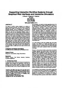
Induction The goal of the induction step is to receive a representation of the workflow from analyzing the workflow log. Depending on the structure of the mined workflow InWoLvE can use two different intermediate data models. Stochastic final automat (SFA) [Her01] can only be used if the described workflow is sequential, i.e. if there are no parallel activities. Since this is hardly sufficient in real world scenarios InWoLvE uses stochastic activity graphs (SAG) [Her01] to represent the extracted workflow. In this chapter we will only use the SFAs for depictions of the data structure because they are easier to understand. Operating in a class four scenario adds to the normal mining process the additional problem of distinguishing between activities of the same name. InWoLvE solves this by searching for a mapping from the activity instances in the workflow log to the activity nodes in the workflow model, using the SplitPar algorithm. The search space is composed of all the possible mappings with the most general model ( only one activity node for all activity instances with one name) at the top and the most specific mapping ( bijective mapping between activity nodes and instances ) at the bottom. Between the other mappings exists a partial order, according to their degree of specialization ( more /less special than). Figure 2.2 shows a graphical representation of the search space. The search algorithm searches top down, starting with the most general model. More special models are generated by splitting activity instances of the same name

9

2.3. THE INWOLVE WORKFLOW MINING TOOL workflow instances B

B

C

C

B most general SFA C C

B

B

B

B

B

C

C

C

C

C

C

B

B

B

B

B

B

C

C

C

C

C

B

C

C

C

C

C

B

B

C

C

most specific SFA

more specific

C

Figure 2.2: The search space for the induction algorithm (adapted from [Her01])

according to different characteristics. Currently InWoLvE implements the SplitCause and the SplitHistory options, which are explained in [Her01]. The split is implemented by dividing the activity instances mapped to one activity node into two groups, according to the characteristic used to locate the split. In the more specific SAG generated by this step, different activity nodes are assigned to the groups. An easy way to implement this is to rename the activity instances in one group, and then generate the next SAG. In the example shown in figure 2.3 the activity instances with the names A and C of the original workflow log are split into A, A’, C and C’ using two split operations. During this process the search is guided by the log likelihood (LLH) per sample of the SAG, as a measure for improvement. Only results that improve the LLH more than a given threshold are returned as results. The search stops if no more nodes are found, or the calculation time is up, whichever happens first. In order to compute the log likelihood, a stochastic sample is used. That is to say that every workflow-instance appears as often as it has been observed. Each of these instances is then tested against the current SAG, and the probability of the examples fitting the model is calculated.

10

CHAPTER 2. BACKGROUND original workflow log A

B

C activity graph G1

B

B

transform to SAG

A

A

A

C

A

C

C

B

A

split

modified workflow log A

B

C’ activity graph G2

B A

transform to SAG A’

C

A

C

B

B

C’

C

A’

A

A’

Figure 2.3: The split operation (adapted from [HK03b]) Transformation The SAG produced by the induction algorithm is very hard to read and structured quite differently from the models used by workflow applications. In the transformation step the SAG is translated into a block-structured workflow-model in the ADONIS format ADL (Adonis Definition Language), which will be described in more detail in section 2.4. The transformation phase can be subdivided into three main steps, explained in detail in [Her01]: 1. The analysis of the synchronization structures of the workflow instances in the workflow log, 2. the generation of the synchronization structure of the workflow model and 3. the generation of the model. However not all SAGs have an equivalent ADL representation. This has two reasons: • There are SAGs that describe an infinite state space ( they might be seen as unbound petri nets ), while well-defined ADL workflow models always describe a finite state space.

2.3. THE INWOLVE WORKFLOW MINING TOOL

11

• Well defined ADL models require properly nested splits and joins - this is also called a block-structure - while SAGs allow any kind of dependency structure. Even though the transformation algorithm aims at coping with these problems in various ways [HK03a], the result of changes in the SAG may trigger unpredictable modifications on the ADL.

2.3.3

Configuration

The induction algorithm is controlled by a number of parameters. Since those parameters are of some importance to the experiments in chapter three, we will in this chapter give a short explanation of the more important ones. timeLimit nrOfBeams

minImprove

nrOfSamples

noiseLevel

the total time the calculation may take. the number of beams used during the beam search. The larger the number, the more paths are simultaneously searched for solutions. this is the minimal amount a new model needs to score higher in the LLH than the previous one in order to be returned as result. Setting this too high may lead to a calculation without results. the number of workflow instances to be used in the induction step. Of course a higher value promises more exact results, but the calculation may then become very time consuming. this parameter sets a threshold for the probability of a branch, below which it is removed from a graph. This is used to eliminate branches that were deduced from the log of rare behavior ( e.g. error by an employee). Of course, setting this value too high may mask an important but very rare event in a workflow.

A complete in depth explanation of the parameters can be found in [Her01].

2.3.4

Restrictions

The current implementation of InWoLvE has some restrictions in learning special models. A lengthy discussion of examples of these restrictions can be found in [Her01] and is beyond the scope of this work. However we give a short list of model properties, that may lead to wrong results: • nested loops or loops that contain alternative branches

12

CHAPTER 2. BACKGROUND • loops containing parallel branches • branches with a local maxima of LLH • very long parallel branches, especially if one branch has a longer processing time than the other • identical activities in short parallel branches

In some cases an experienced user is able to deduce the correct result from a wrong one. Sometimes however the resulting model is totally misleading. Another restriction of InWoLvE is inherent in the system. Since InWoLvE only processes log entries, it obviously can only extract actions that are logged by the system. It is the task of the workflow mining expert, together with the business process engineer, to fill these gaps in the resulting workflow model. Furthermore InWoLvE doesn’t distinguish splits and joins by their semantics ( i.e., AND or OR). Finally, the additional problem of condition mining [AGL98, Her01, vdAvDH+ 03] is not addressed in InWoLvE.

2.3.5

Available data

Although InWoLvE returns only the mined workflow models as result of the calculation, there exists other useful data in the system. Since we will later on use this data at different stages, we will now introduce it and explain its context.

Log Likelihood (LLH) The log likelihood is a measure for the quality of a model. It is calculated before the transformation takes place, and is based on transition probabilities in the SAG structure. The calculation of the LLH has already been described in section 2.3.2.

Split Cause The information about the reason for splitting one vertex into two in the induction phase is stored in the SplitCause variable. This may for example be the different history of two events with the same name, indicating that they represent two different action vertices in the model.

2.4. ADONIS

13

Search Tree In figure 2.2 we introduced the search space for the induction algorithm. Every result produced by the learning algorithm can be found using one of the paths in this search space. The search tree consist of all the paths that lead to results. There exist different paths to a result, however we can distinguish the paths by marking the edges between the results with the split cause that leads to the new result.

Visit count The edge probabilities shown in the results of InWoLvE are calculated on the basis of the number of times a edge has been visited in all the traces used to learn the model. This information, and the visit count for vertices exist in the InWoLvE data structure, but are not displayed in the current build.

2.4

ADONIS

ADONIS [JKSK00] is a Business Process Management Toolkit developed by BOC GmbH. It is of relevance to our project because of two reasons: 1. As mentioned above InWoLvE doesn’t include a visualization component, but instead exports its models to ADL format. Those models are then displayed using ADONIS’ layout component. 2. InWoLvE uses the Adonis Definition Language as model language. Thus the restrictions this language entails for the workflow model are of great interest to us. The visualization component won’t be presented in this chapter, we will however point out some of its weaknesses in chapter 3 since they point us towards requirements for the design of our own layout component. We will now give a short overview over the restrictions imposed by the ADL on the structure of a workflow model.

14


As we already mentioned, models defined in the ADL are block-structured. InWoLvE uses a slightly modified semantic of ADL, described in [Her01]. We will now summarize the restrictions imposed upon our workflow models by this modeling language: 1. there exist exactly one process start and process stop vertex 2. all vertices can be reached from the process start vertex 3. the process stop vertex can be reached from all vertices 4. the graph is connected ( in conclusion of the last two points ) 5. the vertices between a split and its corresponding join form a subgraph. There are no edges, neither inbound nor outbound, connected to vertices that are not member of the subgraph 6. the branches of a split are not connected amongst each other 7. process start, activity and join vertices have exactly one successor 8. split and decision vertices have at least one successor 9. the process start vertex has no predecessors 10. the process stop vertex has no successors 11. the sum of a vertices outgoing edges’ probabilities equals the sum of the incoming edges’ probabilities ( Kirchhoffs’ second law) These restrictions are especially significant, since some of the concepts developed in chapter 4 rely on the reduced graph structure they imply.

Chapter 3

Requirements analysis The goal of this chapter is to find all requirements that a Workflow Mining tool should meet in order to support the interactive aspects of the mining process. Our first step is describing the work with the Workflow Mining tool InWoLvE and trying to solve a number of workflow mining tasks. The problems we encounter during this work will point us directly to requirements for an interactive Workflow Mining tool. Next we evaluate other tools developed in this research area and try to find similarities and ideas that we missed in our approach. Up to this point our whole analysis is focused on practical aspects. We then explore the theoretical possibilities by evaluating methods dealing with interactivity in the related research area of data mining. We finish the chapter by summarizing the requirements found, and by sorting them according to their relevance from a user’s point of view.

3.1

Workflow Mining with InWoLvE

We begin this section by describing step by step the interactive aspects of the Workflow Mining process. We describe for each step how we perform it using InWoLvE and ADONIS, what problems we met during the process and what additional features would be useful for a user. We then describe some of the conducted experiments that led to interesting results. First we show some examples of working on a sufficiently large number of examples, leaving the special problems that arise when working with a too small number of log entries to the following section. To conclude the experiments we work on 15

16

CHAPTER 3. REQUIREMENTS ANALYSIS

a model that can’t be learned due to the restrictions of InWoLvE mentioned in section 2.3.4.

3.1.1

Interactive aspects in the Workflow Mining process

In this section we introduce those steps of the Workflow Mining process that require an interaction of the user with the Workflow Mining tool. We explain the purpose of each step, and show how it is handled by the current working setup of InWoLvE and ADONIS. Based on problems we met during our work with this setup and general observations we made, we then deduce requirements for an interactive Workflow Mining tool.

Choosing the initial parameters The first interaction of the user is needed even before the actual mining process has begun. In order to start the mining process a first set of parameters is needed. The correct settings are highly dependent on two aspects: • the size and complexity of the workflow being monitored • the amount and quality of the available log-data The task of adapting the settings according to first aspect is based on the experience of the user as well as external knowledge about the workflow. Tool support for this task is not feasible at the present state of the art. A Workflow Mining tool can however provide some useful information by extracting the following data from the workflow log without performing a complicated calculation: 1. total number of traces 2. number of different traces 3. an estimation of the maturity of the log by setting 1. and 2. in relation to each other. Such an estimation will, however be too pessimistic if the model contains a lot of parallelism and thus allows a lot of different traces from the same workflow model. 4. an estimation of the complexity of the workflow: average number of events per trace

3.1. WORKFLOW MINING WITH INWOLVE

17

In the current working setup this information is not made available to the user. Thus we state the obvious requirement: All readily available data (i.e. no calculation is needed to extract it) about the workflow log has to be extracted and presented to the user.

Evaluating the results The next interactive aspect of workflow mining is the evaluation of the results. The main task for the user in this step is to examine the results, understand the mined workflow models and get an impression of the calculation’s success. Furthermore he must establish if unexpected aspects of the result models are based on real facts ( for example an unknown action in the workflow ) or if they are errors. In the current working setup InWoLvE writes its results into a text-file after finishing the calculation. As we described in section 2.3.2 the result of one calculation consist of a number of models, marking the path in the search tree according to the chosen parameters. For evaluation every single one of these results has then to be imported into ADONIS for visualization. The first non satisfying characteristic of this working process is the absence of a means to follow a calculation’s progress. Thus the user can neither estimate the quality of the ongoing calculation, nor does he know how long it will take until the calculation is finished. Especially when mining complex models or a large number of traces it is very tiresome to wait half an hour only to realize at the end of a calculation that the results are worthless because of wrong parameter settings. On a very basic level this could be solved by displaying the remaining time of a calculation. This, however still leaves the risk of a worthless calculation. What we need is the possibility to examine the intermediate results of a calculation as soon as they are produced. Display intermediate results of the calculation as soon as they appear. By implementing this feature alone the problem isn’t solved though. The user is still in the position of a helpless observer, without any means to influence the calculation (apart from killing the process). He needs to be able to alter the parameters of the calculation as well as directly stop it if it shows no promise. Enable the user to alter the parameters of an ongoing calculation or to cancel the calculation altogether. When the calculation is finished the next step is to import the results into ADONIS for visualization. Performing this action for every model in the calculation proved to be time consuming, and interrupted the actual process of Workflow Mining by

18


several minutes of repetitive mouse clicking. A tool designed for Workflow Mining has to avoid this by providing an integrated display component. Provide a display component as an integrated part of the tool. Once the results are imported into ADONIS the user has to examine the models and get an impression of the calculation’s success. Because this step depends heavily on the mined workflow, we will examine it based on examples in the next section. At this point a difficulty should be mentioned that we encountered independently of the mined workflow: Even when mining a workflow of only average complexity we received a significant number of intermediate results. During the examination of the models we often switched between them for comparison and to retrace the calculation step by step. In ADONIS the only way to distinguish the models is to systematically assign them names on import. Apart from the fact that it takes a lot of discipline to perform this task effectively, the option will no longer be available if we fulfill the requirement for integration of a display component. Based on our observations we state the following requirement: Provide a clearly arranged overview of the models which: • distinguishes the models from one another • ranks the models according to their history • allows direct access to the models

The final task of accounting for unexpected aspects of the mined models is once more based on external knowledge, and cannot be supported on a tool basis. Based on the information in this chapter the user now has to decide if he will modify the parameters and start another calculation, or if he chooses one model as a final result.

First possibility: modifying parameters for the next iteration If the user comes to the conclusion that his settings for the algorithm can still be improved, he will modify the parameters accordingly and start a new calculation. Again the actual task of modifying the parameters depends only on the skills of the user, and cannot be supported by a tool. Yet there is also an administrative aspect of the task, that only becomes obvious when performing some iterations. If a modification has proven to be wrong, the user will in some cases not want to base the next modification on the last configuration, but on a previous one. Also if coming back to a workflow after some time the user will in most cases not remember the last


19

settings he used. Because of these problems we state the following requirement: Manage configurations in a way that they can be associated with a calculation, enabling the user to choose the configuration that was used to obtain a specific model.

Second possibility: choosing a result model If the user is content with the result of a calculation he has to decide which model to use as a final result. We will explain the difficulties of this step in the next section, based on examples.

Saving the results of the work After the mining process itself is finished there are still two aspects to take care of. The first is that in order to utilize the resulting model, we need to be able to export it in a way that it can be used by other workflow systems. Provide an export mechanism to interface with external workflow tools Furthermore we want to be able to pick up a mining process where we left it the last time. Thus on exiting the system we need to store all needed information. This requirement is present in almost every modern software and is generally referred to as project support. Provide project support, enabling the user at any time to save the state of the project, and to continue at a later time.

3.1.2

Experiments

We start this section by describing the acquisition of the log data used for our experiments. Then we describe some of the conducted experiments that led to interesting results. First we show some examples of working on a sufficiently large number of log traces. Next we focus on the special problems that arise when mining a workflow log that doesn’t provide enough information given the complexity of the model. This experiment represents a situation which is often met when mining young system, where only few traces are available, and the user can’t be sure if the data is sufficient to produce reliable results. To conclude the experiments we work on a model that can’t be learned due to the restrictions of InWoLvE mentioned in section 2.3.4.

20


Acquisition of Log Data Since the principal capabilities of InWoLvE have already been established [Her01, HK03b] we will omit mining known models and focus on more meaningful experiments on unknown models. The data used during these experiments was generated by two test persons for the PHD thesis of Joachim Herbst [Her01]. In order to increase the probability of receiving significant models, the following modeling rules were stipulated: 1. All models are supposed to contain parallel activities (problem classes 3 and 4). 2. The majority of models should contain non unique activities (problem class 4). 3. At least half of the models should contain loops. 4. In every model the unique activity nodes should outnumber the non unique activity nodes. 5. The probability of entering a loop should not exceed 0.2. 6. Two occurrences of the same activity should distinguish themselves sufficiently by their context. 7. Parallel branches should be short. Rules one to three guarantee ample complexity while the other rules try to keep the complexity within manageable limits. In total fifty test models were generated, half of which were used during our experiments.

Mining model es26: Layout deficiencies This experiment was based on traces generated from model es26 which is shown in figure 3.1. Due to the nested structure of this model, it is one of the most difficult to learn in the whole test series. Apart from its complexity it is interesting, because it produces a lot of models in one calculation, and reacts very sensitively to a change of parameters. We started the mining process by using standard settings that produced good results in most cases. Due to the complexity of the model we had to adapt the parameters several times before we received structured results. We then began the process of evaluating the results by leafing through the models in order to get an overview. Already during this step we encountered the first difficulties with the layout mechanism in ADONIS.


21

Figure 3.1: Model es26 In figures 3.2 and 3.3 we show two successive results of our calculation. The only difference between the two models is that in figure 3.3 the loop around the vertices B and D is rolled out, and a new Vertex B is introduced. It is, however not easy to locate this difference at first glance, because the layout engine of ADONIS changes the position of five vertices and as much as eleven edges from one model to the other. Some of the modified edges aren’t even connected to vertices that changed their position. We try to show the extent of the changes by marking all moved vertices and edges in figure 3.3. It is obvious that a workflow mining tool should offer better support for the comparison of successive models. A first step would be a layout component that is more resistant to changes and will provide a more similar layout for successive models. The most important features of such a layout would be: • vertices that exist in both models don’t change their position • new vertices are inserted in a way that causes the least changes in the model • only edges that are connected to vertices that changed their position may be modified These characteristics describe an ideal solution that will be hard or even impossible to reach, especially because there exist other constraints for the layout component as we will see later in this section.

22


Implement a layout component that is resistant to changes between two models. If we only implement the new layout component, the task of locating the actual differences will still be left to the user. An advanced support mechanism would therefore be to compute the differences between two models and mark them for easier recognition. We leave the discussion of how to best display such a comparison to the concept chapter. Offer the possibility to automatically compute and display the differences between two models. Our next step after getting a general impression of the results was to examine the more promising models in greater detail. The underlying difficulty in this step is to understand the structure of the workflow in order to grasp its meaning. Once again we found the layout capabilities of ADONIS quite insufficient for our needs. We would wish for a layout component with stronger emphasis on the structure implied by the syntax of our workflow modeling language ( see section 2.4): • The process start is always performed before any other part of the workflow. It should therefore displayed “above” all other components of the workflow • The process stop is always performed after any other part of the workflow. It should therefore displayed “beneath” all other components of the workflow • The branches of a decision vertex are separate execution possibilities. They should therefore be easily distinguishable in the layout. • The vertices between a split and its corresponding join form a separate subgraph. This substructure should be emphasized by : – layouting the branches to be easily distinguishable, similar to the branches of a decision – treating the split and join similar to the process start and stop – treating the split/join block as if it were one vertex In figure 3.4 we show examples for the first two aspects where the layout produced by ADONIS should be improved. Another aspect of structure is that it will only be recognized if it is always presented in the same way. For example, we are used to see a tree structure presented with the start element at the top. Another presentation will require an adaptation in the thinking of the user. We should for example decide if a decision vertex is placed between its branches or at one side of them, and stick to that decision. Likewise all other aspects of the layout that leave room for decision, need to be decided on at one point.


Figure 3.2: Model es26: Mining Result containing a loop

23

24


Figure 3.3: Model es26: Mining Result without loop. Unnecessarily moved parts of the layout are marked.


(a) Bad separation of paths

25

(b) Overlapping of split block with external structure

Figure 3.4: Deficiencies in the structure of the ADONIS layout

The layout must convey the structure of a workflow by: • emphasizing the structure implied by the syntax of our modeling language • substantiate the structure by eliminating random influence

After the examination of the models we came to the conclusion that one of two models shown in figures 3.2 and 3.3 must be the correct result. In order to opt for either model we first consulted the LLH (see section 2.3.5) for each model, which is calculated by InWoLvE, but stored in an separate file from the models. In many of our other experiments this data was sufficiently significant to make a decision. In this case, however, we needed to additionally consult the search tree structure (see section 2.3.5) to establish that the model without the loop is an improvement of the model containing the loop. Since the LLH and the search tree structure have also proven useful in other experiments we state the following requirement:

26


Display the following data in a way that it is easily available to the user during the mining: • the LLH for the current model • the search tree structure that led to the model

Mining model es9: semantic equality In this experiment we opted for a result model directly after the first calculation. The chosen model was, however, visually different from the solution, as can be seen in figure 3.5. When examining the differences we realized that in our model two splits are combined into one with probability marked branches. Although the visual differences between the models are quite obvious the interesting question at this point is: can one of the models produce traces that the other can’t produce? Or, in other words, do they describe the same workflow on a semantic level? This question is of special interest when the Workflow Mining technology is used to perform incremental workflow design. In this case the question if the new workflow model is mightier than the old one, and which traces can’t be performed with the old model are of central importance. In this rather simple example it didn’t take us long to realize that our model is semantically mightier than the original model, because the loop in the lower part of the graph contains both paths of the decision vertex. A calculation with other parameters later produced the correct result. When dealing with large models it won’t be as easy to perform the comparison without tool support. We therefore state the following requirement: Provide a tool to estimate the semantic similarity of two models.

Mining model es3: syntactic errors In some cases InWoLvE produces results that contain syntactic errors. Two of these errors can be seen in the result of mining model es3 which is shown in figure 3.6. The first error is the split containing only one vertex. Although this is no grave error it reduces the readability of the model. The second error is worse, because it will corrupt any simulation of the model: for


27

Figure 3.5: Model es9 solution, and wrong result

unknown reasons InWoLvE will in some cases assign a very low probability to the first edge in the model. This would cause a great number of simulation runs to abort before actually performing the simulation. It is therefore necessary to: Correct syntactic errors in the result models These errors are caused by InWoLvE, and might very well be solved in the next version. Therefore will not give this requirement priority at this stage.

Figure 3.6: Erroneous structure in model es3

28


Mining model es29 with insufficient traces: problems in recognizing the correct results This and the next experiment simulate working on a young growing system. In this scenario there will most often exist too few traces to perform a reliable mining for a model of a certain complexity. We conducted the experiments by starting with the mining on one trace, and then increased the number of traces step by step. For each step we performed the whole process of Workflow Mining up until the decision for one result. The mining of model es29 showed the interesting effect that only two traces were sufficient to produce a model from which one could deduce the final result. The only weakness of the model was that all loops were rolled out. Beginning with ten traces we then received the correct result, including accurate handling of the loops. However, the calculation didn’t stop at this model, but instead continued and produced overly specific results again. Only when working on more than two hundred traces did InWoLvE reliably stop at the correct solution. The only worthwhile conclusion from this experiment is that the decision for the correct result is even harder when performing the mining on a very small number of traces. Neither this observation nor the fact that loops aren’t reliably recognized when only few traces are mined can be used to deduce a requirement. The surprising fact that only two traces were sufficient to mine all paths of the model brings us to the conclusion that the chosen model was too simple for this type of experiment. We thus decided to once again use model es26, because of its complexity.

Mining model es26 with insufficient trace: reliability of results With this experiment we wanted to apply the scenario of the last experiment on a more complex model. The first consequence of the higher complexity was that all calculations with less than five traces resulted in overly complex models without any recognizable structure. Mining more than five traces produced well structured results that already resembled the actual model. However, some paths were missing, probably because they just hadn’t been visited in the first few traces. The results of the next incremental steps between 20 and 100 traces contained these paths, but were too complex, since loops and decisions were badly recognized. Only the use of 500 and more traces reliably led to the solution. This leads to two conclusions. One is the need for a measure for the reliability of a current model. The measure should in some way estimate the risk that an important

3.2. EVALUATION OF OTHER WORKFLOW MINING TOOLS

29

path has been missed, thus giving an indirect measure for the maturity of the mined system. We will discuss ways of achieving this goal in section 4.5. Develop a measure for the reliability of a model in view of the risk of having missed important paths. The second conclusion is that when we are dealing with very low numbers of samples, an increase of samples will not always lead to better results right away, but instead will only add complexity at first. Although this conclusion is interesting for the methodology of Workflow Mining, we see no way in which a tool could influence it. The two characteristics we observed during this experiment are of great relevance for the work on real systems, where some activities might only happen once every year. The requirement for a reliability measure should thus be assigned a high priority, even though a “normal” user won’t put it at the top of his wish list.

Mining model es14: dealing with the restrictions of InWoLvE As already mentioned in section 2.3.4 some models can’t be learned because of restrictions in the current implementation of InWoLvE. An example of this is model es14 where the result of the mining process is especially poor, as shown in figure 3.7. The problem in this situation is that a user will notice from evaluation of the result models and the other measures proposed by us in this section, that the result of the mining is of very low quality. Because he doesn’t know that this is not due to a wrong setting of his parameters, but a shortcoming of InWoLvE he will then continue to modify the settings, and probably give up in frustration after a number of tries. In this situation it would be sufficient to signal the user that it is impossible to obtain a correct result for the processed log-file. This is not possible, however, because there exists no special symptoms that indicate this special case. Therefore we cannot state any requirements that address this problem.

3.2

Evaluation of other workflow mining tools

In this section we give a short overview of other tools in the research area of workflow mining. Every tool and its underlying concept is introduced, and evaluated in regard to its support of interactive workflow mining. We are interested in concepts we missed as well as in ideas for meeting the requirements we found in the last section.

30


(a) Wrong result of calculation

(b) Correct model

Figure 3.7: Results of learning model es14 Since the mining process itself is embedded in an iterative development cycle as shown in figure 1.1, another interesting aspect for us is, in how far tools can support iterative improvement of workflows in a real world scenario.

3.2.1

The Audit Trail Mining Tool (ATMT)

Maxeiner, Küspert and Leymann propose the usage of Workflow Mining for partially automated construction of process models [MKL01]. In their approach a WFMS is run in a special fashion to acquire first workflow traces, or as they call it, audit trails. In the course of their work they developed a first implementation of their concepts in form of the Audit Trail Mining Tool. The first step in working with the ATMT is to choose the data to be used for the mining process. In contrast to the InWoLvE tool, ATMT directly accesses the database of the WFMS. This seems to be a good way to implement a direct cooperation of a workflow mining and a workflow management system. One must, however, take into account that this type of interface has to be implemented separately for every WFMS, because every system features its own database structure. We won’t state this feature as a requirement for our tool at this point, because in our opinion it is rather an advanced feature, and can be neglected at this stage.


31

When the user has chosen his data source he is presented with some statistics about the log-file, rather similar to the ones we proposed in section 3.1. The user then has the possibility to choose a subset of the data according to timestamps, and to set a parameter similar to the noiseLevel in InWoLvE which controls a mechanism for cleaning the data from erroneous traces. After starting the tool the user has to wait for the calculation to finish before he can import the resulting model into the WFMS of his choice. In the scenario described in the paper the model is then further improved and corrected by the user, before it is used as basis for the next iteration. In summary, ATMT offers roughly the same level of support for interaction with the user as InWoLvE. The user can control the mining itself only through a set of parameters and then has no further possibilities of influencing the outcome of the calculation. The improvement of the resulting model in the WFMS used to display it, is not in the focus of this work since it rather belongs to the area of workflow design, and can be provided by any of the currently available WFMS systems.

3.2.2

Balboa

The balboa system introduced by Cook and Wolf [CW98a, CW98b] is designed as a framework for Workflow Mining applications. Apart from an architecture that allows abstraction from the actual data-sources and tools for the management of this data - both of which are not of direct interest to our work - the current distribution of balboa also includes tools for the analysis of the log-data. The first method for analyzing log-data is the actual Workflow-Mining, provided by the so called process discovery tool and a visualization component, the process model viewer. Both components are only frontends for command-line tools, and offer no more support for interaction than InWoLvE or ATMT. Especially annoying is the fact that the process model viewer offers no means of moving vertices around, or modifying the layout in any other way. This deprives the user of the possibility to adapt a layout to his needs and thus makes it more difficult for him to understand the displayed model. To avoid this problem we declare an additional requirement for our layout component: The user must be able to modify the layout of the models in the display component. Although the process discovery tool is the only tool beside InWoLvE able to work on class two problems, we found no special requirements resulting from this fact. The second means of analysis is the validation of an execution trace against a model, representing the only approach that we found in any of the tools to esti-

32


mate the quality of a mined model. The result of the validation is a measure for the correspondence of the model and the trace. To achieve this the tool compares the expected event stream and the execution event stream, and calculates how many inserts and deletes would be necessary to remove the differences. During this process every action is weighted, for example an insert may be awarded a higher penalty than a delete, because an important event might be missed. Interestingly this definition of validation implies that a difference between the model and an execution trace is generally acceptable. In our opinion, however, if a trace cannot be validated against the model either the trace is wrong, or the model is still incomplete. On this basis even one difference between model and trace seems unacceptable, since it might indicate an important error in the model. Apart from this conceptual difference two other aspects of this implementation kept us from adopting the approach for our tool. First a measure based on only one trace is in our opinion not reliable enough to convey any significant meaning. Second, and more important the comparison is based on an “ expected behavior of the model”. How this behavior is defined in respect to parallel paths and loops in a model is not specified. Thus the result of the validation depends for example on how many times we expect a loop to be processed, i.e. on a random assumption.

3.2.3

MiMo, Little Thumb and EMiT

With MiMo ( Mining Module ) [Med], Little Thumb [WvdA01] and EMiT (Enhanced Mining Tool) [Med] the research group around Wil van der Aalst has implemented three different workflow mining algorithms. All tools are based on petri-net technology, and work on class one and three scenarios. Despite the very different appearance of the tools, they basically all share the same workflow that consists of successive execution of the mining step and an optional display of the results. While Little thumb doesn’t feature a visualization component, EMiT can present its results using a static display. Even though this display component doesn’t have any interactive features, it is still interesting because of its clustering mechanism. In contrast to the other tools EMit displays actions as two vertices, representing the start and end of the action. In its display component those two vertices are grouped to show their relation, as shown in figure 3.8. Although we display actions in one vertex, the visualization method itself might be interesting for structuring large workflow models, for example by grouping the vertices in a split/join block. It could be even more useful if the resulting clusters could be folded and unfolded. Provide graphical clustering of substructures (e.g. a split / join block) in order to increase the readability of models. An advanced feature would be the optional folding and unfolding of the clusters.


33

Figure 3.8: Clustering in the EMiT visualization component

MiMo is implemented as a module of the ExSpect1 tool, and uses the display capabilities offered by its framework. During the evaluation of the tool, we found no aspects of it with relevance to our work.

3.2.4

Conclusions

In summary we note that none of the existing Workflow Mining tools is designed for a high grade of interaction with the user. In most cases the only interaction of the user is the setting of the parameters. Apart from the mining component most tools only offer an additional display component that can be called optionally. Only balboa offers any further possibility of analyzing the mined model, in form of its validation component. Working with these tools thus consists of successive repetitions of mining and evaluating the result. One reason for this fact is that all of the tools introduced in this chapter were mainly developed as a proof of concept for the corresponding mining algorithm. They were not designed for usage in a real world scenario. The second reason is that the additional complexity of InWoLvE caused by the processing of logs of complexity class two and four induced many of the requirements we found in section 3.1. It is only logical that tools that don’t face these problems offer no concepts to deal with them.

1 ExSpect

is short for EXecutable SPECification Tool and is a trademark of Deloitte & Touche

34

3.3


Relevant techniques from Data Mining

In this section we evaluate the related research area of data mining for ideas and techniques that might be applied in our scenario. We start this section by determining the position of workflow mining in the data mining process. This information is then used to narrow our search for techniques down to the most promising ones, which are then evaluated in respect to technical applicability. Finally we test some tools for support of interactive processes.

3.3.1

Sorting workflow mining into the data mining process

In this section we try to fit the workflow mining technique into the more general context of data mining using the CRoss Industry Standard Process for Data Mining (CRISP-DM) [Rei02]. The typical life cycle of a data mining project is shown in figure 3.9. It consists of six phases that will typically be performed more than once, and not necessarily in the sequence shown in figure 3.9.

Figure 3.9: Phases of the CRISP-DM reference model In the following, we outline each phase briefly, and state its relation to our work. Business understanding The focus of this initial phase lies on understanding the project objectives and requirements from a business perspective. This knowledge is then converted into a

3.3. RELEVANT TECHNIQUES FROM DATA MINING

35

data mining problem which can be solved with existing methods. In our case this task has been solved by the researchers [Her01, MKL01, CW98b, vdAWM02] who realized that data mining can be adapted to work on workflow logs. It is thus of no more interest to us. Data understanding and Data preparation In these two phases the data is collected and analyzed in respect to quality problems and structure, before it is prepared for the mining process. These tasks include a visual evaluation of the data, table, record, and attribute selection as well as transformation and cleaning data for modeling tools. Finally the data may have to be converted into the right format. The problems that arise in data mining during this phase don’t apply to our scenario. Modeling In this phase modeling techniques ( e.g. decision trees ) are selected and applied and their parameters are calibrated to optimal values. Typically, there are several techniques for the same data mining problem type. Although we only use one modeling technique, namely the workflow mining algorithm introduced in [Her01], the other tasks in this chapter are very important in our scenario. Therefore we will evaluate this phase in detail in the next section. Evaluation The starting point for this phase is a model that appears to have high quality from a data analysis perspective. The key objective of the evaluation phase is to establish that no important data has been missed during the creation of the model. At the end of this phase, a decision on the use of the data mining results should be reached. This phase corresponds to the decision phase in our mining process. The definition addresses a problem similar to our above stated requirement for a measure for the reliability of a result. We will therefore address it in more detail in the next section. Deployment In the deployment phase the result of the mining process is put to use by the customer. It often involves applying live models within an organization’s decision making processes, for example in real-time personalization of Web pages or repeated scoring of marketing databases. The complexity of this task may vary greatly depending on the objectives. Even though this phase has already been processed in real world applications of InWoLvE, it has not yet been thoroughly analyzed, and is not within the scope of

36


this work. In summary the two most interesting phases for us seem to be Modeling and Evaluation. In the next section we will present the known problems in these areas, and evaluate the techniques used to solve them.

3.3.2

Evaluation of relevant techniques

Modeling According to CRISP-DM the modeling comprises the following tasks: 1. Select modeling technique 2. Generate test design 3. Build model 4. Assess model Tasks one and three are addressed in depth in other research papers [Her01, vdAvDH+ 03]. A modeling technique that has proved to be closely related to our own, is the learning of decision trees. Especially problems of interactivity and presentation during this process are similar to the ones we encountered. Therefore, we will later on evaluate a tool that implements this feature. The generation of the test design can be seen as a preparation for the assessment of the model in task four. For example, in supervised data mining tasks such as classification, it is common to use error rates as quality measures for data mining models. Therefore the test design specifies that the dataset should be separated into training and test set, the model being built on the training set and its quality estimated on the test set. During the assessment of the model the following techniques can be applied: • Test result according to a test strategy (e.g.: Train and Test, Cross validation, bootstrapping etc.). We receive error rates as a measure for the reliability. • Create ranking of results with respect to success and evaluation criteria. • Get comments on models by domain or data experts. Only the first two techniques are relevant for use, since we are looking for software concepts ; although the knowledge of domain experts is certainly valuable if you can afford to pay for it.

3.3. RELEVANT TECHNIQUES FROM DATA MINING

37

The calculation of error-rates seems to be a very good way in order to receive a negative estimation of a model’s quality. Together with the positive measure of success criteria, in our case the LLH, it should give us sufficient data to estimate the reliability of a result. Implement calculation of error-rates for the models as one possible solution for a measure of a model’s reliability. We already stated the requirement for a ranking of the results in section 3.1, therefore this requirement needs not to be treated at this point.

Evaluation In contrast to the previous evaluation steps this one assesses the degree to which the model meets the business objectives and seeks to determine if there is some practical reason why this model is deficient. This work currently has to be done by the workflow mining expert with the help of domain experts, because it requires knowledge that is not logged in the system. All we can do is to think about ways to support the expert in this work. A first step might be a comparison of a designed workflow with the result of the mining step in order to better estimate the differences. This requirement was already stated in an early section. Additionally one might wish to see the log entries that induced a certain action in the workflow. This would make it easier to explain differences between the modeled and the real workflow. Since these aspects are not in the core focus of this work we won’t treat them with a high priority. Implement a method to show the log-entries that caused a certain activity.

3.3.3

Tools

In this section we first take a look at CART [Sys], a tool specialized in learning decision trees. As we mentioned above, the problem of interactively learning trees is interesting for us, because it addresses similar problems as Workflow Mining. As a second tool we evaluate SPSS 11.5 as a substitute for the class of complete data mining tool kits.

38


CART CART is a sophisticated data mining tool specialized on decision tree learning. Especially interesting for us is the so called Navigator window shown in figure 3.10, which enables a user to browse through the results of a calculation. This display method meets the requirement of CRISP-DM to create a ranking of results, and at the same time it can be used to implement a history of the calculation.

Figure 3.10: The CART Navigator dialog Although interactivity in CART only consists of choosing a result after the calculation is finished, the design of its UI still points into the right direction. A component similar to the navigator can be considered a useful addition to a workflow mining tool. Therefore we state the following requirement as a suggestion for the design of the GUI for a workflow mining tool: Implement the requirement for a ranking of the results that induces an order on the results, similar to the Navigator dialog in CART.

SPSS 11.5 As a representative for the many available data mining tool kits we chose SPSS for two reasons. The first is that since the company participated in the development of CRISP-DM the product should meet the requirements stated there. The second

3.4. SUMMARY OF REQUIREMENTS

39

reason is that in contrast to the main competitor Clementine and SAS Enterprise Miner there exist trial versions of SPSS 11.5. We started the evaluation by following the examples in the tutorial and then tried to experiment with the software. The results of the evaluation were disappointing. Neither is there explicit support for the CRISP-DM process, which would have narrowed our search, nor did we find any special support for interactive work during the mining process. Due to the enormous complexity of the toolkit it wasn’t possible to evaluate all of its functionality. By following the tutorials we tried to get a general impression of the tool. It might be possible that we missed some decisive feature in this process.

3.4

Summary of requirements

In this section we group the requirements that we gathered in the last few sections. Additionally we sort them according to their importance from a user’s point of view. We introduce priorities from P1 to P3, where P1 is absolutely necessary, P2 is important and P3 stands for a “nice to have” requirement. Additionally we grouped the requirements according to which problem is addressed by them. In summary an interactive workflow mining tool has to meet the following requirements; 1. Support efficient work with the tool. P1 provide a display component as an integrated part of the tool P1 display intermediate results as soon as they appear P1 enable the user to alter the parameters of a calculation, or to cancel the calculation altogether P3 the tool should be able to interact with a workflow application; a very efficient possibility would be direct access to the database of a workflow system 2. Support the user in understanding the results of a calculation. P1 develop a special layout component that implements the following features : – the layout of successive models contains as few changes as possible; the ideal solution would provide the following features: ∗ vertices that exist in both models don’t change their position ∗ new vertices are inserted in the way that causes the least changes in the model

40

CHAPTER 3. REQUIREMENTS ANALYSIS ∗ only edges that are connected to vertices that changed their position may be changed – the layout must convey the structure of a workflow by: ∗ emphasizing the structure implied by the syntax of our modeling language ∗ substantiate the structure by eliminating random influence P1 user must be able to modify a layout in the display component P3 syntactic errors in the result models are automatically corrected P3 large models can be clustered in order to make them less complex P3 provide method to show the log-entries that caused a certain activity 3. Support the user in the decision for a final result. P1 develop a measure for the reliability of a model, possibly based on the calculation of error-rates P1 show LLH and search tree structure for the model P1 offer possibility to automatically compute and display the differences between two models. P2 provide a tool to estimate the semantic similarity of two models 4. Support a smooth workflow especially during work on complex models. P1 provide a clearly arranged overview of the models in a way that: – – – –

distinguishes the models from one another ranks the models according to their history allows direct access to the models resembles the CART Navigator dialog

P1 provide possibility to undo unsuccessful calculations P1 manage configurations in a way that they can be associated with a calculation P2 it should be possible to work on projects using the following features: – it is at any time possible to save the current state of a project, including all results that have been calculated up to that time – likewise it is possible to restore any saved project

Chapter 4

Concepts Some of the requirements that we collected in the last chapter are only implementation issues. These will be addressed separately in chapter 5. In this chapter we look at those requirements that first have to be analyzed in order to find concepts for their solution.

4.1

Support of a smooth workflow in the mining process

In this section we introduce our concepts to support a smooth workflow during the mining process. In detail we have to meet the following requirements: 1. provide a clearly arranged overview of the models 2. manage configurations in a way that they can be associated with a calculation 3. provide the possibility to undo unsuccessful calculations 4. implement project support Of these requirements the fourth is only an implementation issue and will not be explained in depth. To fulfill the first requirement we must also take into account the functional requirements that we deduced during the requirements chapter, namely the overview concept must distinguish the models from one another, rank them according to their history and allow direct access to any model. During the evaluation of the Data Mining tools in section 3.3.3 we realized that the navigator component of the CART tool addresses all of these aspects. Thus we 41

42

CHAPTER 4. CONCEPTS

decided to place a component in the user interface that depicts the results similarly to the CART Navigator dialog. To this end we need one property of the results for each of the two axes in a diagram. The property on the y-axis should be a measure for the quality of the result. Since the LLH is the only such measure we currently have, this choice is clear. The property for the other axis should identify the results. One possibility would be to simply number all results as they occur, thus using time as the property for the yaxis. The drawback of this solution would be that we would have a lot of repetition, because the first intermediate results of most calculations are the same. This would lead fast to an unmanageable amount of data. We thus need an additional id, that distinguishes the results from one another. This id can then be used to remove repeating results. Using the LLH is not possible, since there may exist two different results with the same LLH. As a solution we distinguish the results by the path in the search tree through which they were reached (see section 2.3.5). Since sometimes there exists more than one path to a model some results may still occur more than once, but according to their search history they are not the same. A screenshot of this component is shown in figure 4.11, together with the results of the validation component that we will introduce in chapter 4.5. This still leaves us with the problem of managing the configurations that were used to calculate the results. In this case the simplest solution also seems to be the best one. We recommend associating each model with the first configuration that was used to learn it. This way the user can choose a model through the component described above, and then access the corresponding configuration. With the association of model and configuration we also solve our last problem, the undo function for complete calculations. It can now easily be implemented by deleting all models that share the same configuration.

4.2

Support efficient work with the tool

We deduced the requirement to design the tool for efficient work from problems that occurred during our work with InWoLvE. Considering that all of the functional requirements which we gathered in this context can be solved on an implementation basis we won’t list them here again, however, because these requirements are basic guidelines for the development of a workflow mining tool, they are relevant for some of the concepts introduced later in this chapter. In case one of the requirements influenced a design decision we will point this fact out.

4.3. LAYOUT - THE MAXIMUMRECOGNITIONLAYOUT ALGORITHM 43

4.3

Layout - The MaximumRecognitionLayout Algorithm

The functional requirement for a special layout algorithm was stated as a part of the requirement to provide support for the user in understanding the results of a calculation. We decided to treat it separately, however, because of its complexity. Thus we introduce in this section the MaximumRecognitionLayout algorithm, which was developed according to the requirements described in section 3.4. Based on these requirements we are faced with two separate problems to be solved by the layout algorithm. 1. generating a well structured layout for the workflow model, that helps the user in understanding the described workflow 2. generating layouts for successive results with maximum similarity. The first problem is currently only addressed by tool manufacturers, under the aspect of layouting a manually created workflow model for demonstration. However the layout produced by the tools we evaluated was in no case as structured as we would wish. Due to the management background of many of these tools, they rather offer a good looking first suggestion of a layout, that can then be fine tuned for presentations. Not surprisingly, the only solution working on the same data model as we are, is the one provided by the ADONIS tool, which already has proven to be quite insufficient for our special requirements. The second problem has already been investigated by a number of authors [BETT94, Bra01], and we will give a brief overview of the current state of the art in this research area in the next chapter. During the final assessment of those methods we will show that none of the existing algorithms can be applied to our problem immediately, because of our basic conditions. As a consequence of the two problems just mentioned and their implications for a possible implementation, we decided to develop a special layout algorithm to suit our needs. We will introduce the developed algorithm, by presenting the basic principle of the algorithm in section 4.3.2. We then develop concepts from our requirements in section 4.3.3, as a basis for the explanation of the algorithm in chapters 4.3.4 to 4.3.6. Finally we try to estimate how well the developed algorithm meets the requirements.

44

4.3.1

CHAPTER 4. CONCEPTS

Dynamic Graph Layout - State of the Art

The ad hoc solution for dynamic graph layout is to use a static layout algorithm, and just animate the transition from one layout to the next [DGK01]. As Diehl, Görg and Kerren already pointed out [DGK01], this approach has some serious drawbacks. The layouts of two successive graphs may confront the user with two completely different results, even if only some small changes occurred. The fact that the user can see the transition between these two layouts doesn’t support him in keeping a “mental map” of the graph [ELMS91]. This is however exactly what we need to do, in order to fulfill the requirement of recognizability. Another simple approach to the problem is to forbid changes to vertex positions, once they have been placed [Bra01]. It is obvious that using this approach we would not be able to maintain any structure in the layout when new vertices are inserted. This conflicts with our requirement for a concise and well-structured layout. Out of the vast number of layout algorithms [BETT94] we are only interested in those with a special capability for dynamic layout. We will try to give a brief overview of the different approaches in this field, and evaluate them with respect to our requirements. Finally, we will explain why none of the existing algorithms is sufficient to solve our dynamic layout problem.

Incremental Layout One possibility for layouting successive graphs is to take the layout of the preceding graph as a basis for the new layout. North proposes a method where the relation between two layouts is made by building the graph step by step [Nor96]. To this end the algorithm accepts changes only as elemental insert or remove operations of vertices and edges. It then tries to find an appropriate adaptation of the layout for each change. For example the insertion of a vertex might best be solved by introducing a new level into the graph and putting the new vertex in that level. A similar approach is proposed by Miriyala, Hornick and Tamassia, but with a special focus on the “orthogonal graphic standard” [BETT94], where edges are only drawn rectangularly. The special problems that apply to this approach are only of little interest to us. The algorithms of this class seem promising for our project. They are however all based on incremental changes that don’t occur in our data model. Because every model is the result of a transformation as mentioned in section 2.3.2 we are instead presented with completely new graphs for every change. This means, that in order

4.3. LAYOUT - THE MAXIMUMRECOGNITIONLAYOUT ALGORITHM 45 to apply one of the above mentioned algorithms we would first need to calculate the differences between two graphs, and then split them up into the allowed operations. In conclusion we note that the class of incremental layout algorithms holds promise for our application field, but can’t be applied in the implementation without putting further work into our data model.

Foresighted Layout A completely different approach to dynamic graph layout is to calculate a “global” layout, which induces a layout for each of the n graphs, as proposed by Diehl et al. [DGK01]. The special characteristic of these layouts is that neither the edges nor the vertices change their positions in the subsequent graphs. In order for this to work, the layout algorithm needs to know the “future” of the graph, that is the next n-1 changes. Obviously this need for the future to be known is the drawback of the proposed method, since it makes online layout near to impossible. Another problem special to our approach is, that the changes are not presented step by step as taken for granted by Diehl [DGK01]. Instead we get whole graphs from our algorithm, and would thus need to use a search algorithm, in order to find the corresponding vertices of the same name in the subsequent graphs. Of course we may hope that in most cases the predecessors or successors may distinguish the vertices from one another, but in graphs with long paths this may be an expensive calculation. Another possibility would again be to calculate the differences between two graphs, and feed them to the algorithm as elemental operations. As already mentioned above, this task is a whole new problem in itself, especially since it would require the implementation of another search algorithm. Furthermore the results for the first few graphs in a long series may look a bit strange, since edges flow around vertices that are not yet visible, and vertices are scattered all over the drawing area. An example of this is shown in figure 4.1 The reasons mentioned above lead to the conclusion that the proposed algorithm doesn’t meet our requirements. Especially the requirement of layouting the results during the calculation conflicts with the need to have all results at hand. We might try to calculate a global layout while still receiving new results. However, this would mean that the layout would change with every new result, thus destroying the advantage of this approach altogether. Despite the drawbacks of this approach for layouting the results during the calculation, it could be used when the calculation has finished, or when a user wants to review all results up to the current one. In this case the algorithm should provide much better layouts than the MaximumRecognitionLayout algorithm ever could.

46

CHAPTER 4. CONCEPTS

Figure 4.1: An example of foresighted graph layout. Other approaches A method for visualizing the effects of split and merge algorithms on a graph is introduced by Robbins, Jeffery and Robbins [RJR00]. It includes a layout mechanism that is optimized for dealing with the changes that may occur when applying a split or merge operation. As promising as this may seem, given that the nature of the SplitPar algorithm is that of a split algorithm, we still can’t use it in our application. As mentioned in section 2.3.2 the SplitPar algorithm doesn’t split vertices of our graph. It works on the log data, where a split of one example might imply a lot of changes in the graph. For obvious reasons this multitude of possible changes wasn’t taken into account during the development of the algorithm.

Assessment As we have seen above, for technical reasons none of the currently existing methods can be used to solve our dynamic layout problem right away. Furthermore, most of the introduced approaches only deal with the changes, and still need a static algorithm to perform the basic layout. This implies that we would in any case need to design an algorithm that can convey the structure of the business model to the viewer. For this reason we decided to develop an algorithm that can deal with the dynamic aspects of the layout, and at the same time provides a static layout fit for workflow models. To this end, we will in the following chapter develop concepts for a new layout algorithm. For the mentioned reasons this algorithm will neither use incremental

4.3. LAYOUT - THE MAXIMUMRECOGNITIONLAYOUT ALGORITHM 47 nor foresighted layout techniques. It will thus basically be a static layout algorithm that will try to find a change-resistant layout with the help of a well defined set of constraints. This is possible because we can make use of the restrictions imposed on the graph by the ADONIS definition language, as described in section 2.4.

4.3.2

Basic principle of the MaximumRecognitionLayout algorithm

As with a lot of layout algorithms [BETT94] we will divide the layout area into levels and columns, and try to find the best positions for the vertices. This process can be split into three steps 1. Calculating the level for each vertex 2. Setting the column for the vertices 3. Refining the layout in respect to edge-crossing and overlapping These three steps are described in the chapters 4.3.4 to 4.3.6. During these steps we need to take into account the requirements defined in 3.4. In order to do this in a well-defined way, and prevent misinterpretation of requirements, we first deduce a set of rules from the requirements in section 4.3.3, and build our design decisions on this rule set. During the next few chapters the algorithm is described based on a vertical layout. In order to better describe the layout process we will then use left, right, up and down to describe the location, although one could easily change the orientation by swapping columns and levels. Furthermore although the models don’t represent trees, we chose to call the different paths in the graph branches, since it better conveys the intended meaning. For an explanation of the special semantic implied by the different vertex types in ADONIS see the short explanation in section 2.4.

4.3.3

Deduction of a set of rules for the algorithm

In this chapter we will deduce a set of rules from our requirements stated in chapter 3.4. We will try to create a direct link between one requirement and the rules used to fulfill it.

Requirement: change resistance In detail the requirement for a change resistant layout consists of three functional requirements:

48

CHAPTER 4. CONCEPTS • vertices that exist in both models don’t change their position • new vertices are inserted in the way that causes the least changes in the model • only edges that are connected to vertices that changed their position may change

Each of these requirements is based on dynamic information, e.g. the differences between a model and its predecessor. Since we decided for a static approach we have no access to this kind of information. As a consequence, we can only try to provide a good approximation of these requirements. To this end we will in this and the following sections state rules that define the correct layout very exactly, and thus guarantee a maximum resemblance of the business process models. Furthermore there is one aspect of the changes that we can deal with. A very common change between two successive models is the introduction or the removal of a loop respectively. The ideal way to deal with this change is to ignore the loops during the calculation of the layout. To this end we introduce the following rule: R1 Ignore edges that are part of a loop during the calculation of the layout. How these edges can be located will be explained in section 4.3.4. The located edges can then be drawn after the calculation of the layout has been finished. Unfortunately, in most cases the introduction of a loop into a model is accompanied by other changes like the vanishing of the vertices in an until then rolled out loop. Nevertheless the above mentioned rule has proved to be effective in preventing changes, as may be seen in figure 4.6.

Requirement: emphasize the structure implied by the syntax of a workflow When we stated this requirement in section 3.1.2 we listed in detail what functional requirements have to be met in order to fulfill it. We will now deal with these requirements step by step, and explain how we can meet them with our rules. We start with the requirement to place the process start- (stop -) vertex above (beneath) the other vertices. This requirement can obviously be translated directly into the following two rules: R2 The process start vertex is always placed in the top level. R3 The process stop vertex is always placed in a separate level below all other levels.

4.3. LAYOUT - THE MAXIMUMRECOGNITIONLAYOUT ALGORITHM 49 The next requirement was that the branches of a decision vertex should be easily distinguishable. To this end we introduce rule R4: R4 Each branch of a decision is treated as a separate substructure with the maximum with of the branch. Thus if one branch has a breadth of three columns, all vertices in the next branch can only be placed in column four and above. Thus we effectively separate the branches. Finally we stated the requirement that a split / join block has to be treated as a separate subgraph. To this end we adapt the rules R2, R3 and R4 for usage in split / join blocks and state the corresponding rules R5,R6 and R7: R5 The split vertex is placed in a level above its successors. R6 The join vertex is placed in a separate level below those of its predecessors. R7 Each branch of a split is treated as a separate substructure with the maximum with of the branch. The third part of the requirement demands that a split/join block is treated as one vertex, and should not overlap with external structure. Overlapping can only occur if the split is either nested in another split/join block or if it is placed in one branch of a decision. Because of rules R4 and R7 it is in both cases guaranteed that the block gets its width reserved, and can’t be overlapped by external structure.

Requirement: eliminate random influence Another requirement was to eliminate random influence on the layout. In order to achieve this we need to specify rules for those aspects of the layout that are as yet unspecified. The first unspecified aspect are the columns in which to place the process start and process stop vertices. In case of the process start vertex we are free to decide for a position, thus we choose the first column ( from left to right ). Because this is a trivial task we don’t state it as a rule. We will deal with the process stop vertex later in this section, because its placement is important for the conciseness of the layout. Next we need to decide where to place the decision and split vertices: either centered between its branches or to either side of them. Like the placement of the process start vertex this is only a question of taste. This decision can safely be

50

CHAPTER 4. CONCEPTS

left to the implementation, on condition that the placement for one vertex type is always the same. The last aspect of the layout that is as yet undefined is the ordering of a decision or split vertices’ successors. To eliminate this randomness we state the following rule: R8 The successors of split and decision vertices are sorted according to a welldefined key. Of course there are several possible choices for the key of this ordering; 1. the length of the path to the corresponding join, or, in the case of decision vertex, to the process stop vertex 2. the probability of the path 3. the type of the vertex 4. the name of the vertex, or a generated identifier For an implementation of the first key we would need to perform a calculation for every path. In large models this might lead to poor performance. The second possibility works only for decision vertices, and some special cases where branches of a split are marked with a probability. In contrast the data that is needed for the third and fourth key is statically available for every vertex. Therefore we propose the usage of a combination of the third and fourth key. More details on this follow in section 4.3.4. A disadvantage of rule R8 is that after its application the most common solutions for minimization of edge crossing and overlapping cannot be be applied any more, because these methods work by changing the position of a vertex in its level [Bra01].

Requirement: concise layout Since every part of a graph that is not visible because of overlapping is lost information for the user, it must be the goal of every layout algorithm to produce a concise layout. This general requirement has to be dealt with in addition to the requirements we stated in section 3.4. Since we can only deal with this requirement within the restrictions imposed by the rules stated above, we only found two approaches to fulfill it:

4.3. LAYOUT - THE MAXIMUMRECOGNITIONLAYOUT ALGORITHM 51 The first method concerns edges overlapping vertices. This is the worst fault, since the vertices are the main carrier for information. As mentioned above we cannot apply the common solution of moving the vertices in a level in order to reduce edge crossings, because of rule R8. As a compromise we resorted to drawing the edges around intermediate vertices. An example of this may be seen in figure 4.5. R9 Edges are drawn around intermediate vertices The second approach is to place the stop vertex in the way that promises the least possible edge crossings. We therefore state rule R10, although it is somewhat in contradiction to the requirement for elimination of random influence on the layout. R10 Place the process stop vertex in the way that promises the least possible edge crossings.

4.3.4

Arranging the vertices in levels

The algorithm starts by sorting the vertices into levels. This is done using a breadthfirst search [Sch97] on the graph. During this search we number the vertices in the order that they are visited, and assign them their levels. The result of this step is depicted in figure 4.2. In this step we realize the rules R2, R3, R5, R6 and R8, as described in the next few paragraphs. Rule R2 is automatically fulfilled by using the process start vertex as first vertex in the breadth-first search. We just assign it level number one, and all other vertices will be placed in subsequent levels. In the same way rule R5 is automatically fulfilled, since all successors of a split vertex are automatically placed in a new level. In order to fulfill rule R6 we need to make sure that the level of a join vertex is set via the longest path towards it. We accomplish this by adjusting the level of the join vertex every time when it is reached over a longer path. Thus, instead of stopping a calculation path when hitting a visited vertex, we check if it would put the vertex in a deeper level. In some cases the successor of the join vertex may already have been run through the algorithm. This would mean that the join vertex is placed in a lower level than its successor. In order to prevent this we need to modify all vertex levels that were calculated on the basis of the old level of the join vertex. We can do this by again adding the join vertex to the queue. In order to prevent endless iterations, we need to make sure that during a recalculation of levels only those paths are used that were used to set the level during the first calculation. This can simply be achieved by remembering the predecessor when setting the level for the first time.

52

CHAPTER 4. CONCEPTS

Figure 4.2: Result of organizing the vertices into levels. This special treatment of a join vertices is the reason why in figure 4.2 the join vertex (number nine) is located in level six instead of level five. After calculating the levels for all vertices we make sure that rule R3 is fulfilled by putting the stop vertex in a separate level, if it isn’t placed in the deepest level. Finally it is easy to modify the breadth-first search, to process the children in sorted order, thus implementing rule R8. In the prototypical implementation we used the following order: • The different vertex types are ordered by the following priorities: 1. split vertices 2. decision vertices 3. action vertices • Join vertices are placed in the same column as their corresponding split vertex. • Process start and stop vertices have a level of their own, hence they don’t need a special priority. • Two vertices of the same type are compared by a generated string identifier. In the case of an action vertex the identifier is its description, and in the case

4.3. LAYOUT - THE MAXIMUMRECOGNITIONLAYOUT ALGORITHM 53 of split and decision vertices the type and the description of their successors. If this identifier is equal, the comparison can be stretched to the next level.

In listing 4.1 you can see an implementation of this part of the algorithm in pseudocode. Listing 4.1: Sorting the vertices into levels Procedure c a l c u l a t e L e v e l s ( V e r t e x r o o t V e r t e x ) ; levels [ rootVertex ] = 0 ; q u e u e . add ( r o o t V e r t e x ) ; w h i l e q u e u e n o t empty c u r r e n t V e r t e x = p o p F i r s t E l e m e n t ( queue ) ; children = getChildren ( currentVertex ); sortVertexArray ( children ); for each c h i l d V e r t e x ∈ c h i l d r e n i f not v i s i t e d c h i l d V e r t e x levels [ childVertex ]= levels [ currentVertex ] + 1 ; { set the predecessor to the vertex that sets the depth for t h i s vertex } childVertex . predecessor = currentVertex ; enqueue ( c h i l d V e r t e x ) ; mark c h i l d V e r t e x v i s i t e d ; else { s e t s t o p and j o i n v e r t i c e s a c c o r d i n g t o l o n g e s t p a t h } if levels [ childVertex ] < ( levels [ currentVertex ] + 1) { j o i n v e r t i c e s can be p u s h e d d e e p e r by any v e r t e x n o r m a l v e r t i c e s can o n l y be p u s h e d d e e p e r by t h e predecessor that set t h e i r l e v e l the f i r s t time } i f ( c u r r e n t V e r t e x i s J o i n V e r t e x ) or ( childVertex . predecessor == currentVertex ) levels [ childVertex ]= levels [ currentVertex ] + 1 ; enqueue ( c h i l d V e r t e x ) ; end i f end i f end i f end f o r setRootVertexToLowestLevel ( ) ; end w h i l e

This part of the algorithm is similar to Dijkstra’s algorithm [Sch97] for computing the shortest path to the vertices in a graph, only that it’s looking for the longest path.

54

CHAPTER 4. CONCEPTS

4.3.5

Computing the column of the vertices

The second important part of the layout algorithm is the calculation of the paths’s width, and the assignment of the columns. For that purpose the algorithm traverses the graph in a depth-first search, while recursively calculating the width of the segments and setting their position at the same time. We will explain this step in detail a bit further down. First we show the algorithm’s conceptual mode of operation.

Figure 4.3: Schematic split of the graph into subgraphs during the calculation. As you can see in figure 4.3 the algorithm starts by splitting the graph into subgraphs. The width of each of those subgraphs is calculated and passed on upwards. You will find the width of a subgraph in the top left corner of the rectangle surrounding it. The value it passes on is noted just above that. As you will see, the first split has an internal width of two, but will pass on a width of three, thus setting the width of the left path to the correct value. The goal of this step is to assign each path of the graph its maximal width, thus implementing rules R4 and R7. For this calculation the following precepts apply: • A visited vertex always has a width of zero. • The process stop vertex has an initial width of one. • A normal vertex passes the width of his successor on. If the successor has already been visited the vertex will return one instead.

4.3. LAYOUT - THE MAXIMUMRECOGNITIONLAYOUT ALGORITHM 55 • A split vertex, its corresponding join vertex and all intermediate vertices are seen as a separate subgraph. The algorithm first calculates the width of this subgraph. Afterwards it starts the calculation on the join’s successor. It then returns the maximum of the successor’s width and the width of the join vertex. • A decision vertex returns the accumulated width of its successors.

Figure 4.4: Calculation of width and position We still need to set the positions of the vertices. It is obvious that this can be achieved in the same traversing as the calculation of the width. For this purpose, we only need to assign each vertex its column when the calculation of its width starts. For children of decision or split vertices we need to increment this start column with every processed child. In figure 4.4 you can see a schematic depiction of this calculation. The arrows pointing down are the positions, handed to the vertices by their fathers, whereas the arrows pointing up represent the width of the respective vertex. Above the arrows the chronological order of the steps is noted. When taking a closer look at figure 4.4 you will notice that, after processing the split, the sequence differs from that of a normal depth-first search. The reason for this is the already mentioned special treatment of splits as subgraphs. In order to provide this feature, we first calculate the width and position of all vertices between the split and its join. We then return the maximum of the “internal” width and the width of the join’s successor.

56

CHAPTER 4. CONCEPTS

By marking visited vertices we can locate and then ignore loops during this calculation, thus implementing rule R1. In listing 4.2 we show a pseudo-code implementation of the algorithm.

4.3.6

Refinements

The goal of the final step of the layout algorithm is to implement a concept for preventing edge crossings and overlapping of edges and vertices as far as possible. To this end we will realize rules R9 and R10, as described in this section.

Figure 4.5: Complete layout of the example graph Our concept for preventing edges from overlapping vertices is to draw them around intermediate vertices and edges. We can achieve this quite easily by looking at all vertices that have an outgoing edge connected to a vertex in the same column, and more than one level deeper or higher. All we need to do then is check if there exists a vertex in an intermediate level. All the data we need for this step is the location data computed in the previous steps. We still have to implement R10, and find the placement for the process stop vertex that causes the least edge crossings. Here we can make use of two special properties of the layout algorithm. The first is that by using a breadth-first search for sorting the vertices into levels, the vertices are ’pulled’ upwards, due to the “greedy” nature of the algorithm. The second effect is, that by setting the column of a vertex

4.3. LAYOUT - THE MAXIMUMRECOGNITIONLAYOUT ALGORITHM 57 according to the first edge connected to it when traversing in a depth-first search, we push the vertices to the left. Because of the first property of the algorithm the best position for the process stop vertex is in the column of the shortest path connected to it. Like this we can be sure that there is the least possible number of vertices direct above the vertex. The second property leads to the conclusion that when there is more than one shortest path, we take the column of the one furthest to the right. One can observe this very nicely when comparing the layout of the graph in figure 4.4 where the process stop vertex is positioned in the column of the longest path, and the layout in figure 4.5 where the vertex is positioned according to the shortest path. In the second layout we averted the edge crossings present in the first one. In some cases their still might occur edge crossings. For example a model might still contain edge crossings if the shortest path contains a split with a large number of paths. The result of applying the complete algorithm on the example graph may be seen in figure 4.5. Listing 4.2: Calculating the width and setting the positions of vertices. Function i n t setColumnReturnWidth ( Vertex c u r r e n t V e r t e x , Vertex fatherVertex , int offset ); c u r r e n t C o l u m n = f a t h e r V e r t e x . column + o f f s e t ;

if is visited currentVertex i f currentVertex . f a t h e r . l e v e l >= fatherVertex . l e v e l c u r r e n t V e r t e x . column = c u r r e n t C o l u m n ; currentVertex . father = fatherVertex ; endif return 0; endif c u r r e n t V e r t e x . column = c u r r e n t C o l u m n ; currentVertex . father = fatherVertex ; i f currentVertex is ProcessStopVertex return 1; e l s e i f c u r r e n t V e r t e x i s A c t i o n V e r t e x or J o i n V e r t e x or P r o c e s s S t a r t V e r t e x childWidth = setColumnReturnWidth ( c u r r e n t V e r t e x . child , currentVertex , 0 ) ; r e t u r n maximum ( c h i l d W i d t h , 1 ) ; else i f currentVertex is DecisionVertex children = getChildren ( currentVertex ); totalWidth = 0; currentOffset = 0;

58

CHAPTER 4. CONCEPTS

for each c h i l d V e r t e x ∈ c h i l d r e n t o t a l W i d t h + = setColumnReturnWidth ( childVertex , currentVertex , currentOffset ); currentOffset += 1; endfor else if currentVertex is SplitVertex correspondingJoinVertex = findJoinForSplit ( currentVertex ); { c a l c u l a t i o n w i l l s t o p when i t h i t s t h e j o i n V e r t e x } internalWidth = setColumnReturnSplitBlockWidth ( currentVertex , correspondingJoinVertex ); successorWidth = setColumnReturnWidth ( correspondingJoinVertex , correspondingJoinVertex . father , 0 ) ; r e t u r n maximum ( i n t e r n a l W i d t h , s u c c e s s o r W i d t h ) ; endif

4.3.7

Assessment

Since an intensive test of the algorithm is beyond the scope of this work we will at this point provide a discussion of the degree to which the four main requirements addressed in section 4.3.3 are met.

Requirement: change resistance An application of the layout algorithm on the scenario from which we deduced our requirements in section 3.1.2 shows a perfect result. As we can see in figure 4.6 the layout is totally resistant against the introduction of the loop. This kind of change is the simplest example, because there occur no other changes but the introduction of the loop. In some cases, however, the SplitPar algorithm will produce successive models with completely different structures. It is impossible for a static layout algorithm to perfectly deal with such extensive changes. An example for this can be seen in figure 3.5 where the SplitPar algorithm merged two split blocks together in one. In these cases the algorithm still provides the same layout for the parts of the graphs that are contained in both results, but fails to keep the complete layout change free. The only complete solution for this shortcoming would be the application of the MaximumRecognitionLayout algorithm in a foresighted layout. However, as mentioned above, this only makes sense after all results have been calculated.

4.3. LAYOUT - THE MAXIMUMRECOGNITIONLAYOUT ALGORITHM 59

Figure 4.6: es26 with and without loop

Requirement: emphasize the structure implied by the syntax of a workflow

This requirement is fully met. Of course it is somewhat subjective to begin with, because another author might argue that a different structure would be better suited for the given syntax. One disadvantage of the algorithm is that by assigning each branch its maximum width, it may in some cases produce a very drawn apart layout. This problem could only be solved by sacrificing some of the clarity of the layout, which would be in conflict with our requirements.

Requirement: eliminate random influence

This requirement is also completely fulfilled, apart from the placement of the process stop vertex. As we explained in section 4.3.3 we decided to place the process stop vertex in the position that promises the least edge crossings, and to thus accept a certain randomness in exchange for a more concise layout.

60

CHAPTER 4. CONCEPTS

Requirement: concise layout For most models the algorithm meets this requirement to our full satisfaction. There exists however one problem that still needs to be dealt with: Very long sequential paths are not displayed in a concise way. The algorithm simply puts all the vertices in one column and draws the edges around intermediate vertices. If there exist many backward edges this results in a complex layout which is hard to understand for a user. We found no way to solve this problem within the restrictions imposed on the algorithm by the other requirements.

Evaluation of performance Since the MaximumRecognitionLayout works in a static way, it has to layout the complete graph for each result, instead of only processing the changes like a truly dynamic algorithm. This leads to a slightly lower performance on large graphs than that of an incremental layout algorithm. This “weakness” is a direct result of the basic conditions that forced us to implement the algorithm as a static algorithm in the first place.

Conclusion Despite the mentioned drawbacks the MaximumRecognitionLayout algorithm has already proven its applicability during the work with the prototypical implementation. It should however be mentioned that applying a similar algorithm on a less structured data model is bound to produce less satisfying results.

4.4

Supporting the user in understanding a model

In this section we develop concepts to support the user in understanding a workflow model. This task is especially important when working with complex workflows where even the original process model may be hard to understand. While the original models are often layouted by hand for better understanding and contain additional documentation, the results of the mining process lack this information. We now present our concepts for providing a replacement for this missing information. Apart from the requirement for a special layout component, which has already been treated in the last section, we stated four more functional requirements to support a user in section 3.4. Of these, only the requirement for the possibility to

4.4. SUPPORTING THE USER IN UNDERSTANDING A MODEL

61

modify a layout manually was assigned a high priority. This is however only an implementation issue, and need not be elaborated on. The other requirements are either not important enough or too difficult to implement them at this stage. Instead we will describe two other concepts, which we developed during our work with the prototypical implementation, and which support the user in the understanding of complex models.

4.4.1

Layout

In section 4.3 we already introduced our own layout component. Besides helping the user in keeping track of changes, the developed component also helps the user in understanding a model by emphasizing the structure of our workflow models, as described in section 4.3.3.

4.4.2

Marking the sections of a model according to their significance

A well known fact in the design of user interfaces is, that the usage of other display methods than just textual notices is often useful to emphasize the meaning of important data [Tuf92, Shn96]. Since the probability of a path being visited is a measure for its significance it is important to convey this information to the user. This measure should however not be based on the local probability of an edge, but instead on its absolute visiting frequency. This is much more significant, because it implicitly includes the predecessors in the evaluation of an edge. For example an edge with a local probability of 1.0 will still be visited very rarely if it is located in a path that starts with an edge of a very low probability. Thus it has a low absolute visiting frequency. We begin by deciding how to display the information. In the second part of this section we then explain in detail how data about the absolute visiting frequency can be obtained, and how the data must be enhanced to be significant. Finally we give an outlook on a measure for the deviation of a learned model from the original one, based on the methods developed in this section.

Design decisions Since the probability is generally associated with the edges, our display method should do the same. We basically saw two methods of marking the edges for our purpose: • change the shape of the lines e.g:

62

CHAPTER 4. CONCEPTS – use thick lines to mark very probable paths and thin lines for the others – use dotted lines for paths that are seldom visited • change the color of the lines

We decided to use color, since in our opinion it is the stronger method. Furthermore until now we haven’t used this means for any purpose, whereas we already use different shapes to distinguish the vertex types. Since it is always better to use a well-known scale than to define a new one, we decided to create a temperature map of the graph as can be seen in figure 4.7. Red colors indicate busy edges and green colors edges that are seldom visited.

Figure 4.7: Temperature coloring of a model graph

Implementation issues There are two ways of implementing this feature. The first possibility is to simply use the visit count that exists for each vertex and edge in InWoLvE as described in section 2.3.5. The visit count denotes how many times an edge (vertex) has been visited in all the traces that were used to learn the model. For our coloring need values between zero and one. Thus we need to normalize the visit count, giving us the absolute visiting frequency PAV F . To compute it we first need to find the edge with the highest visit count CMax. If the model contains loops, this count is higher than the number of traces #Traces. The absolute visiting frequency for an edge ei can now simply be calculated by dividing the visit count of the edge C(ei ) through the highest visit count: C(ei ) PAV F (ei ) = CMax

The second possibility is to perform simulated runs of the model and thus generate an artificial visit count CSim for each edge. The simulation algorithm needed to perform this task has, for example, been implemented in the ADONIS tool, and is

4.4. SUPPORTING THE USER IN UNDERSTANDING A MODEL

63

described in various papers [EW01, HJK97]. When the simulated visit counts are available we can calculate the absolute visiting frequency as CSim (ei ) PAV F (ei ) = CMax Sim

In order to provide statistical significant results the number of simulation runs #Sim has to be very high. For an implementation of the second approach we would have to specially implement the simulation engine in our prototype. Since this is too much work at this stage we decided to use the first possibility in our prototypical implementation. The disadvantage of this approach is, however, that we can only perform it on models we received from the InWoLvE kernel.

Outlook An interesting feature would be to display the differences between the actual visit counts and the simulated ones. We expect the difference between those two numbers to be greater for less good models, thus giving an indirect measure for the quality of the model. The difference should be greater for the parts of the model that do not resemble the correct result, thus indicating what part of the model is probably wrong. To implement this feature we would first need to scale the simulated visit counts down to the number of traces that produced the real visit counts. Then we would need to calculate the difference between the simulated visit counts and the real ones for each edge. We could thus compute the absolute deviation DABS for an edge ei as follows: )×#Traces DABS = |C(ei ) − CSim (ei#Sim |

To display the information effectively, we would then need to normalize it, using the maximum deviation between the real and the simulated visit counts as norm.

4.4.3

Introducing a post-calculation noise-reduction (post-pruning)

Another possibility to clarify the meaning of a model is to fade out paths below a certain probability threshold. Like this the user can better focus on the important parts of a model. In data-mining tools this feature is known as post-pruning.

64

CHAPTER 4. CONCEPTS

As we already mentioned in section 2.3 InWoLvE already performs a similar operation called noise reduction during the calculation. During noise reduction InWoLvE evaluates the available traces and excludes some of them from the calculation, according to the setting of the noiseLevel parameter. This approach has two disadvantages:

• the user doesn’t see which paths have been excluded due to the noise reduction

• the information in the excluded traces is permanently lost. In order to include it in the result models, a new time consuming, calculation has to be performed.

Post pruning solves these problems, because initially all available information is shown, and only gradually hidden as the user increases the threshold. The realization of this concept is fairly easy. Basically we only need to check for each edge if its possibility lies above the current threshold, if not we hide the edge. Then we hide all successors until we either find a vertex that has another incoming edge, which is not hidden, or until we hit the stop vertex. An advanced feature would be to remove decision or split vertices if they only have one path left that is above the threshold. Although this would mean an additional simplification of the model, one should not forget that it makes it harder to compare the pruned graph with the original one. A problem of post-pruning as we described it above is that the resulting workflow models may violate some of the syntactic restrictions of the ADONIS Definition Language which we introduced in section 2.4 and relied on during the implementation of some features. In detail rules one, three, four, six, seven and eleven may be violated, because we don’t correct side effects of hiding edges. For example, if all outgoing edges of a decision vertex are below the threshold this vertex has no more outgoing edges, thus violating restriction number six. If we wanted to use this feature to acquire result models, we would need to implement a continual correction of these syntactic errors. Since we only want to use it as a visual support tool, however, the implementation described above is sufficient. In conclusion this feature is very useful to gain an overview over a complex model, but is not suited to find a final result, because of the reasons mentioned above.

4.5. CREATING A MEASURE FOR THE RELIABILITY OF A MODEL

4.5

65

Creating a measure for the reliability of a model

In this section we try to find a measure for the reliability of a mined model. The measure should in some way estimate the risk that a path has been missed during mining, because it hasn’t been processed yet and thus wasn’t contained in the traces. This risk is especially high in two cases: • in a system where the workflow changes very often • in a young system, where only few traces are available and some actions (e.g. end of a project) have not yet occurred In either case the intended measure will also be a measure for the resulting model’s reliability and maturity. We will now explain our basic concept to develop such a measure, and then explain it step by step.

4.5.1

Basic Concept

In section 3.3 we already suggested to implement the measure based on classification error-rates. Classification is perhaps the most commonly applied Data Mining technique. It uses a set of preclassified examples to induce a model that can then classify other record instances. Fraud detection and credit-risk applications are particularly well suited for this type of analysis. This approach frequently employs decision tree or neural network-based classification algorithms. The use of classification algorithms begins with a training set of preclassified example transactions. For a fraud detection application, this would include complete records of both fraudulent and valid activities, determined on a record-by-record basis. The classifier training algorithm uses these preclassified examples to determine the set of parameters required for proper discrimination. The algorithm then encodes these parameters into a model called a classifier. Once an effective classifier is developed, it is used in a predictive mode to classify new records into these same predefined classes. For example, a classifier capable of identifying risky loans could be used to aid in the decision of whether to grant a loan to an individual. The accuracy of a classifier is defined as the probability of correctly classifying a randomly selected instance. In our case the classifier corresponds to our model, which will classify instances into the two classes valid and invalid. If we use the correct model as classifier all results should be classified as valid, if we ignore corrupted log-entries.

66

CHAPTER 4. CONCEPTS

However, we don’t want an estimation of the accuracy of a model, but rather of its reliability, as regards missed actions or possible changes. We can achieve this by adapting the selection of the test set to our need as we will describe in section 4.5.3. In the rest of this section we will first explain when a trace is valid with respect to a model. Then we define a measure on the basis of classification, before we explain the implementation of the feature.

4.5.2

Validating one trace

Before introducing in detail the possible ways to define a measure on the basis of validation we first need to explain when a trace is valid in relation to a model. Basically the problem we face is to answer the question if our test model can produce the trace we want to validate. In other words, we need to check if the trace is contained in the language described by our model. This question has already been evaluated to some extent for message systems [Rid72] which can be converted into petri nets [Pet81]. However the semantics described in these papers do not match those specified by the ADL (see section 2.4). Therefore we will now explain how to perform this operation on our data model. Theoretically we could generate all possible execution traces for the test model, and then just check if the validation trace is contained in these traces. We face a problem, however, as soon as our model contains loops, because the model can then generate an infinite number of different traces. This problem can be solved by only generating all the traces up to the length of the validation trace. Still this approach can only be called brute force, all the more so, because a model that also contains concurrent paths will produce a huge number of traces. Therefore it is not advisable to really implement validation this way. We basically see two possibilities to implement the validation in a more efficient way. The first is another brute force approach, where all possible mappings of trace action to vertices are tested one after the other. If they represent a valid path through the model we have validated the trace. This method is very efficient if the vertex names are unique (complexity classes one and three), because then only one test is necessary. Because of the same reasons as above, namely loops and concurrency, this test is not necessarily easy. The second possibility is to use an constructive approach, and try to match the actions in the trace step by step to action vertices. This approach seems more promising when we are dealing with models of complexity class two and four, because it excludes impossible matchings. Because of this feature we decided for the second possibility. Therefore we will explain this approach in more detail in


67

section 4.5.4.

4.5.3

Possible measures on the basis of validation

Of course the validation of one trace is not a suitable measure, since its results are too random. There exist various accuracy estimation methods on the basis of validation[Koh95]. We will now give a short overview of the applicable ones.

Holdout The holdout method is the simplest method of measuring validation accuracy. The dataset is partitioned into two mutually exclusive subsets called the training and the test or holdout set. A common partitioning is two thirds for the training set and the rest for the test set. The model is then learned from the training set, and validated against the test set. For the following explanations we define D as the dataset and Dt as the test set. Furthermore we define S(D) as the size of a dataset, and V (D1 , D2 ) is the number of traces successfully validated when using D1 as training set and D2 as test set. Using this definition the accuracy estimation for the holdout method is defined as: t ,Dt ) acch = V (D\D S(Dt )

This measure uses only two thirds of the available data for learning the model. Because of this inefficient use of the data the learned models are less good than those of the other measures, resulting in a rather pessimistic measure.

Cross-Validation In k-fold cross-validation the dataset D is randomly split into k mutually exclusive subsets (the folds) D1 , D2 , ...Dk of approximately equal size. In every validation step one subset is chosen as the test set, and the others are used as training set. The accuracy of the cross-validation method is the sum off all the possible validations divided through the number of validations: acccv =

1 k S(D) Σi=1V (D\Di , Di )

The obvious drawback of this method is the time needed to learn all the different models. Furthermore a different dataset might need different parameters, to get the optimal results. This makes it harder to compare the different accuracies.

68

CHAPTER 4. CONCEPTS

Furthermore the result of cross-validation cannot be associated with a special model. It is thus rather a measure for the quality of the data used for mining, than for a specific model.

Bootstrap The bootstrap method differs from the other methods introduced in this chapter, because although it uses a part of the data as test set, it uses all the data as training set. In data mining this is especially useful when there exists only a very small dataset. However it is this special characteristic that renders the method useless for our needs. Herbst [Her01] has already proven that all traces that are used by InWoLvE to learn a model are included in the result. Thus the bootstrap method would in our case always result in a 100 percent accuracy estimation.

Conclusion For our scenario the holdout method seems to be the only one fitting in with the other requirements. The whole design of the system is aimed at a workflow that provides the information at the same time with the calculation results. This would not be possible with cross-validation since it needs more that one calculation. A drawback of both the cross-validation and holdout is the inefficient use of the data. The only solution would be to use the calculation with validation as an estimation for the reliability, and then use all traces for a complete calculation. This would obviously disturb the user in following the workflow, and additionally it would be very time consuming. Probably the best solution is to use validation until the models are sufficiently promising in respect of the LLH and the reliability measure, and only use a full calculation within the final step.

Selection of the test set As we mentioned above, a problem of the holdout method is the correct selection of the test set. In data mining the goal of the validation is to estimate the accuracy of the model, in classifying the instances. To this end a random selection of the test set is best suited, since it guarantees independence of training and test set. Since our goal is not an estimation of the accuracy, but rather of the reliability, this is not the solution we chose. We want to estimate how stable the learned model is in respect to rare actions or changes in the workflow. An estimation of this can be achieved if we split the dataset according to the start time of the traces. We


69

use the earlier ones as training set and the later ones as test set. As a result of this selection, changes that occurred only in the last few traces can’t be validated against the model learned from traces that didn’t include the changes. Thus the measure will rate them lower, as we will also see in the next section.

4.5.4

Developing a constructive approach for validation

In this section we explain our constructive approach to solve the validation problem. The basic concept of our validation algorithm is to step by step walk a path through the model according to the traces. To this end we first need to sort the action instances in the traces according to their end times. The validation of a trace is done by trying to map the instances time-ordered on the vertices of a model. Every time an instance is successfully mapped onto a vertex we look at the successor of the vertex, and try to match the next instance against it. We now explain the algorithm in more detail, starting with strictly sequential models, which are easiest to understand, and then gradually increase the difficulty. For various reasons we chose to describe the algorithm state based. This also corresponds to our implementation where the state is implemented as a separate class.

Description of the validation state Basically the validation state is only used to store data about the validation process as it proceeds. This data can then be used by the validation algorithm, to control the validation process. Effectively the data itself is not important for the algorithm. It is based on the information that can be extracted from the state. For example the algorithm needs to know if a vertex matches the currently active action instance in the state. If this is decided using a never changing list of action instances and a pointer to the current element, or as we implemented it, a stack which removes each instance after it has been matched, is not relevant. In the following sections we will explain the algorithm based on the data in the validation state, as we implemented it, because this is more transparent than an explanation based on extracted information. The first important data stored in the validation state is the stack containing the action instances to be validated, ordered according to their timestamps first instance on top. The second data is a history of the matched vertices. All other data is only needed for special cases that won’t be explained in detail. Every time an action instance is matched against a vertex the action instance is removed from the stack, and the vertex is added to the list of matched vertices.

70

CHAPTER 4. CONCEPTS

Our algorithm can then at any time be described by the vertex that we observe, the validation state and the action that has to be taken.

Strictly sequential models We first consider a model that contains no decision vertices. We begin by validating the initial state against the process start vertex. Since the process start vertex is always valid, we can continue with its successor. We now have to validate the state against an action vertex (we know there are no decision and split vertices in this model). The validation state is valid with respect to the action vertex if its current action instance matches the action vertex. In this case we can continue the validation with the vertex’s successor. If the state cannot be validated the validation has failed, because there exist no other possibilities to continue. In order to be successful, the validation not only needs to reach the process stop vertex, but also must match all the available action instances. Without the second condition, an endless trace could be modified against a model containing only one action vertex, if only the first action instance is matching. In this very easy case the table describing the algorithm is very simple (n.i. denotes for not important): Vertex Type Process Start Vertex Action Vertex Action Vertex Action Vertex Process Stop Vertex Process Stop Vertex

Match yes(always) n.i no yes yes(always) yes(always)

Nodes Left n.i 0 ≥0 ≥0 0 ≥0

Action continue with successor validation failed validation failed continue with successor validation succeeded validation failed

Dealing with decision vertices only introduces little additional complexity. The validation algorithm simply tries to validate one path after the other. Because each path needs to be validated with the current state, the algorithm makes a copy of the current validation state for each path, and remembers the original state. This procedure is also unproblematic when dealing with loops, as long as the loop contains an action vertex, because there is only a limited number of action instances. If the loop doesn’t contain an action vertex as shown in figure 4.8 this would lead to an endless loop. This can be prevented if we log the visited vertices in the validation state. Using this data, it is easy to locate such endless loops simply by checking if an action vertex was visited since the decision vertex was visited the last time.


71

Figure 4.8: Model that could lead to an endless loop Models containing concurrency The naive approach to validate a split vertex would be to do it analogously to the validation of the decision vertex. The only difference would be that not only one branch must be validated, but all the branches that are assigned a probability of one. This approach is, however, severely flawed because of two reasons: 1. only the sequence of actions on one branch is fixed; actions on different branches may occur in any sequence 2. branches with a probability less than one may be included or not, opening up two separate branches in the calculation space of the validation. Because of the first problem we need to adapt the validation to try all valid sequences of the actions. For example using the naive approach, the model shown in figure 4.9 will wrongly classify the trace A,C,B as invalid. We deal with this problem by using backtracking. Instead of continuing with the successor of a validated vertex, the algorithm has to return the validation state to the split vertex. At the split vertex the state is copied, and passed on to every branch of the model. Since we don’t want to keep on validating the first vertex in a branch, the algorithm needs to pass through all those vertices that have already been validated. A split join block is successfully validated if all its branches with a probability of one and at least one branch have been validated. In figure 4.10 you can see this part of the validation performed on an example. The figure is simplified in so far, that after a match on an action vertex, we directly distribute the cloned state to the successors of the split vertex, instead of first visiting

72

CHAPTER 4. CONCEPTS

Figure 4.9: Negative example for naive validation approach the split vertex. As we can see there exist two possibilities for validating the model in this case. When there exist nested splits, the algorithm always has to backtrack to the outermost split in order to allow for all possible sequences. Because of our second problem mentioned above, we first need to gather all the possible solutions before we continue. Thus we can’t just continue with the successor of the split/join block when we have found the first solution. Instead we need to cache every possible solution, and continue until all possibilities for the split/join block have been processed. The validation of loops in combination with split/join blocks is only problematic in so far as it interferes with the backtracking. Normally a vertex that has been validated will be passed over by the validation algorithm. If the vertex is however the next vertex to be validated in a loop, it may not be passed over. This distinction is made using information that can be extracted from the validation state. For all details of the algorithm take a look at the prototypical implementation in ProTo.

4.5.5

Evaluation of the developed measure

For our implementation of the measure, we chose to define the measure as acc = −1 + acch Like this the values of the measure lie in the same range as those of the LLH, and can be displayed more concise. A typical effect of the application of the reliability measure on a sufficiently large log-file is the bell-like curve of its values as shown in figure 4.11. The explanation for this effect is the nature of the learned models. The first results are very general,


A

B2

B1

D

C

Vertex: Start Vertex Instances: [A,C,B,B,D] History: [] Action: pass on

Vertex: Split Vertex Instances: [A,C,B,B,D] History: [SV] Action: copy state, pass on

Vertex: A Instances: [A,C,B,B,D] History: [SV,SP] Action: match

Vertex: B1 Instances: [A,C,B,B,D] History: [SV,SP] Action: validation failed

Vertex: C Instances: [A,C,B,B,D] History: [SV,SP] Action: validation failed

Vertex: A Instances: [C,B,B,D] History: [SV,SP,A] Action: pass through

Vertex: B1 Instances: [C,B,B,D] History: [SV,SP,A] Action: validation failed

Vertex: C Instances: [C,B,B,D] History: [SV,SP,A] Action: match

Vertex: B2 Instances: [C,B,B,D] History: [SV,SP,A] Action: validation failed

Vertex: A Instances: [B,B,D] History: [SV,SP,A,C] Action: pass through

Vertex: B2 Instances: [B,B,D] History: [SV,SP,A,C] Action: match

Vertex: A Instances: [B,D] History: [SV,SP,A,C,B1] Action: pass through

Vertex: D Instances: [D] History: [SV,SP,A,C,B2,B1] Action: match

Vertex: Stop Vertex Instances: [] History: [SV,SP,A,C,B2,B1,D] Action: validation succeeded

Vertex: B1 Instances: [B,B,D] History: [SV,SP,A,C] Action: match

Vertex: C Instances: [B,B,D] History: [SV,SP,A,C] Action: pass through

Vertex: D Instances: [D] History: [SV,SP,A,C,B1,B2] Action: match

Vertex: Stop Vertex Instances: [] History: [SV,SP,A,C,B1,B2,D] Action: validation succeeded

Figure 4.10: An example walkthrough for the validation of a split

73

74

CHAPTER 4. CONCEPTS

and will thus fit any trace that contains the same actions as the ones used to learn the model, resulting in a high rating in the reliability measure. Next are models, that are closer to the real model, but contain parallelism or decisions that are not yet correct. These models score bad in the reliability measure. The ratings for the models start getting better again as soon as the learned models are more accurate. However, in most calculations the last four or five results all score 1.0 in the reliability results, because they are already sufficiently close to the result.

Figure 4.11: The validation (curve) and history (bars) component

When working with few traces, the significance of the measure depends on the complexity of the model. With simple models few traces are often enough to produce results that validate with 100 percent. With more complex models the measure produces better results in so far as a perfect validation is seldom reached until enough traces are computed. Another aspect of the measure is, that it can be used to estimate the reliability of a mining on a young workflow management system. Since we use the last added traces as test set, the measure responds very sensitively to newly added actions or paths, because the learned model is not able to validate them. Thus a system that is still changing very often, or that hasn’t been run long enough to visit some rare actions will score rather worse, showing the low reliability of the mined model. In conclusion the developed measure is valuable as a negative measure for excluding results. It is, however, less suited to find the best result, because models that are close to the final results often score a hundred percent. Considering the nature of the learned data, this was to be expected, since the models that score one hundred percent are in a way “correct”, they just don’t represent the best solution.

4.6. SUPPORTING THE DECISION FOR ONE RESULT

4.6

75

Supporting the decision for one result

Throughout the gathering of requirements it became obvious that the decision for one result at the end of the mining process is, together with the choosing of the correct parameters, the most difficult task. The measure developed in the last section can be used to exclude some possibilities, but is insufficient to support a decision between models of a certain quality, since they all score the highest values.

4.6.1

Visualizing the LLH and the search tree structure of a model

During our requirements analysis we stated the requirement to display the LLH and search tree structure of a model, because this information can be useful to locate the final result. The search tree structure represents information about how a result was reached in the search tree of InWoLvE. Because the data itself is structured as a tree, it is only natural to display it as a tree graph, with the models as leaves. Since the LLH is a property that is associated with the models, the appropriate place to display it is in the leaf representing the corresponding model. We still can decide if we wish to display information on the edges. The edges represent the transition between the models. Appropriate information would in our opinion be: • the differences between the two models • the cause for the split that created the new model The first is difficult to display in this context, since it would have to be textual information. A list of vertices can hardly be considered useful information. The cause for the split is based on information of the SAGs that are internally used by InWoLvE, which makes the information hard to understand when this structure is not visible. Since both possibilities didn’t convince us, we chose not to use the edges to display information.

76

CHAPTER 4. CONCEPTS

4.6.2

Visually comparing two models

After comparing the semantics of two models, we are now looking for the best method to compare the graphs of two models. From a user interface viewpoint we have basically three possibilities: 1. Display a graph that contains all vertices and edges from both graphs. Vertices that belong only to one of the two graphs are marked in some special way. 2. Only display one graph, and mark the vertices that distinguish it from the other graph. This is an additive comparison of the graphs, since only the additional vertices and edges are displayed, while information about lost parts of the graph is not displayed. 3. Compare both graphs side by side, using the display method from above for both of them.

Figure 4.12: Possible design for the comparison component The possibilities one and three display the same amount of information, while possibility number two lacks half of the information. While it would theoretically be possible to display possibilities one and two in the standard graph display component of our tool, this possibility doesn’t exist for possibility number three, since it needs to display two graphs.

4.6. SUPPORTING THE DECISION FOR ONE RESULT

77

We suggest displaying the comparison of the models in a new component, using either method one or three. A decision that still has to be made is what will actually be marked as a difference between two graphs. For example the introduction of a second path in one graph also implies the insertion of a decision vertex. However, we don’t want the first path to be marked as a difference only because it is now preceded by a decision vertex. The solution is to mark the special vertices that are different (decision, split, join), but to perform the comparison only on the action vertices. An example of how the result of the comparison component might look can be seen in figure 4.12.

Chapter 5

Prototypical Implementation In this chapter we present “ProTo - The Process Tool”, our prototypical implementation of a workflow mining tool. After evaluating possible system architectures we introduce the one we decided for, and explain some interesting aspects in detail.

5.1

System architecture

ProTo can be divided into four logical components: • the InWoLvE kernel • the user interface • the control unit that manages the workflow • the database We will now discuss two possible system architectures on a design level.

5.1.1

Central control using indirect communication

This architecture is based on a central control unit. Its task is to control the different components, and to manage the data flow in the application. Any communication in the system has to pass through this component. As a result of this system design a modification of the workflow can easily be implemented by adapting the control component. 78

5.1. SYSTEM ARCHITECTURE

79

Figure 5.1: System architecture using the system core as central component

5.1.2

Hardwired workflow using the calculation as central component

This architecture doesn’t use a central control component, but instead uses a hardwired workflow. This setup is easier to implement, since there is no need for complex interfaces. The components are independent, and can be started separately. The data is transferred using files.

Figure 5.2: System architecture using the calculation as central component

80

CHAPTER 5. PROTOTYPICAL IMPLEMENTATION

5.1.3

Conclusion

There exist other possible architectures, but they are mainly variations of the two designs shown above. Since we stated in the requirements that a workflow mining tool should be developed as an integrated tool, we decided for the first architecture, because it provides a closer linkage of the components. Furthermore it is more flexible than the second architecture. This more than compensates for the additional implementation complexity.

5.2

Technology evaluation

To implement the system as sketched above we need to find a technology that meets the following criteria: • possible integration of InWoLvE • database access • existing package for displaying graphs Since the first two aspects are fulfilled by almost every modern language / technology we focus our decision on the package for displaying graph structures. The package for graph drawing is especially important because the workflow models displayed by it are the center of our GUI, and also the main purpose of the tool. In the evaluation of the different packages we used the following criteria: • The license: since ProTo is only a prototypical implementation, we preferred a non-commercial product. As we might need special features that are probably not implemented in some packages an open source license would be preferable. • Applicability: this is a subjective criteria that actually is a combination of several aspects. For one, the package should be well extensible, in so far as the displayed objects are representations of our internal model. Also we didn’t want a package that only displays the graphs without the possibility to interactively change the graph. Furthermore the quality of the packages’ display unit as well as a first impression of the API is taken into account. . • Support: here we list the support offered for the packages.

81

5.2. TECHNOLOGY EVALUATION

• Documentation: with this criterion we rate the extent and the quality of the available documentation.

The most important of these measures is the applicability. As mentioned above, the rating is very subjective, and because of the complexities of the packages some features may not have been taken into account. The results of the evaluation are shown in the following table, ordered by qualification for our project. Package JGraph

PL JAVA

License LGPL

App. very good

Support highly responsive forum with big archive

yfiles Graphlet

JAVA C++

very good good

OpenJGraph

JAVA

commercial free for academic use LGPL

Graphviz

C

average

VGJ

JAVA

special open source GPL

commercial none, development stopped low traffic forum very good

poor

poor

GDToolkit

C++

free for academic use, closed source

poor

E-mail

average

Documentation Java API Doc, good examples, commercial documentation commercial manual, examples Java API Doc complete HTML manual, Java API Doc Tutorial, API Documentation

Even though yfiles features the better API, and with the application in ARIS Process Platform [Sch99] has already proven to be fit for the field of business processes, we decided to use JGraph because of license issues. Also the very good support in the web forum of the project was an argument for the open source package. In consequence we decided to use JAVA as implementation language for our tool. The integration of InWoLvE can be done using the Java Native Interface, and the communication with the database will be done using the JDBC architecture. In figure 5.3 we show a screenshot of the ProTo user interface.

82


Figure 5.3: Screenshot of the ProTo user interface

5.3

Introduction of the ProTo system architecture

In figure 5.4 we give a schematic overview of the ProTo system, with respect to technology, component architecture, component interaction and important class names. Based on this overview we will now address interesting aspects of the system.

5.3.1

Separating model and view

The separation of data and presentation is one of the most important paradigms in object oriented software development. In Java it is supported by the MVC ( Model View Control ) Pattern. The ProtoGUI represents the view and the control component, while the ProtoProject class is the model. In its function as controller the ProtoGUI will modify the ProtoProject, which then notifies its view, the ProtoGUI. The actual implementation is a little more complicated than that: The user interface consists of various components, ProtoGUI is only the main component that contains all the others. At system start the components register as change listener with the model. Now, if one of the components changes the model all user interface components will be notified and can update themselves.

5.3. INTRODUCTION OF THE PROTO SYSTEM ARCHITECTURE

83

Figure 5.4: General overview of the System

5.3.2

Integration of InWoLvE

The integration of InWoLvE was one of the most interesting implementation issues. The easiest approach would have been to use InWoLvE as stand alone program, and interface with it using text-files, like it is done in the balboa framework. However since we decided to develop the tool using an integrated design this approach is no appropriate solution. Instead we decided to modify InWoLvE to integrate into our architecture. To this end we needed to fulfill the following tasks : • compile InWoLvE as dynamic link library (dll), and operate it using JNI • design an interface for the communication between InWoLvE and the ProTo components • modify InWoLvE in order to allow interference of the user during the calculation • modify InWoLvE in order to return the results during the calculation instead of at the end

84


Since the first issue is a purely technical matter, and is described in various FAQs, we won’t describe it in detail.

Design the interface between InWoLvE and ProTo The interface between InWoLvE and Proto must on the one hand provide the possibility to control a calculation in InWoLvE and on the other hand transfer the results from InWoLvE to ProTo. To this end we introduced into InWoLvE methods for the start, stop and configuration of a calculation. The transfer of the results is achieved using callback methods, that build the result models step by step, and send a signal to the system if one model is complete. Despite the use of two different programming languages this solution has proved to be very stable, and a lot faster than data transfer using files.

Modify InWoLvE to allow interference during calculation

(a) original sequence

(b) modified sequence

Figure 5.5: Original and modified operation sequence in InWoLvE In figure 5.5 we show the original and the modified operation sequence in InWoLvE. As can easily be seen the configuration was originally only read at the

5.3. INTRODUCTION OF THE PROTO SYSTEM ARCHITECTURE

85

beginning, which made it impossible to modify the configuration during the calculation. Furthermore we needed to find a way to abort a calculation as it was demanded in the requirements. To this end we introduced a method into InWoLvE that enables us to modify the configuration (including the calculation time) during a running calculation. By setting the calculation time to zero we can abort the method during the calculation. Additionally we need to modify the operation sequence in InWoLvE to check the configuration after every iteration, as can be seen in 5.5.

Chapter 6

Conclusion and Outlook 6.1

Conclusion

In this thesis we systematically gathered requirements for a workflow mining tool with special respect to the interactive nature of the workflow mining process. To this end we conducted experiments, evaluated other existing tools and concepts of the related area of data mining for applicability in our context. We then developed concepts to fulfill the requirements based on some guidelines defined during the requirements phase. Among others we developed a special layout algorithm that provides a more structured and change resistant layout than those of current workflow tools. Furthermore we defined a measure for the reliability of mined models based on validation, and devised several methods of supporting the user in the decision for a final result. Most of the concepts were implemented in the ProTo tool in order to prove their feasibility. First working experiences with this tool have been very promising, surpassing the possibilities of a combined system of a non-interactive workflow mining tool and a “normal” workflow tool by far.

6.2

Outlook

A real estimation of the value of the developed concepts can only be made after putting the system to work in a realistic scenario. Also the feedback from nondeveloping users will bring invaluable information about the deficiencies of the tool. From an implementation viewpoint it would be interesting to realize the concepts 86

6.2. OUTLOOK

87

that are not included in the current version of ProTo. Especially the comparison of models should help a user in everyday work. Another option totally ignored in this work would be to modify the InWoLvE tool. For example a more modular implementation of the calculation kernel should make an improved interface with the ProTo tool possible. Furthermore it should be worth an attempt to rise more data during the calculation phase. This would require a systematic evaluation of each aspect of the mining algorithm for available data. In terms of interoperability with other workflow tools, it would furthermore pay off to implement an interface to a more general file format than adl. One alternative would be the common XML format for workflow logs proposed in [vdAvDH+ 03]. Of course this might imply models with a different semantic than the one we based this thesis on. In current research Kleiner [Kle03] is currently developing a tool for his approach on incremental workflow design on the same implementation basis as ProTo. Since the architectures of the tools were carefully designed to be adaptable, an integration should be possible. It will be interesting to see if the application of both methods on one scenario will show any benefits.

Bibliography [AGL98]

R. Agrawal, D. Gunopulos, and F. Leymann. Mining process models from workflow logs. Lecture Notes in Computer Science, 1377, 1998.

[BETT94]

G. Di Battista, P. Eades, R. Tamassia, and I. Tollis. Algorithms for drawing graphs: an annotated bibliography. In Computational Geometry: Theory and Applications, pages 235–282. 1994.

[Bra01]

J. Branke. Drawing Graphs. 2001. Dynamic Graph Drawing, pages 228–246.

[CW98a]

J. E. Cook and A. L. Wolf. Balboa: A framework for event-based process data analysis. In Proceedings of the Fith Inter. Conf. on the Software Process, Lisle, Illinois, USA, pages 99–110, 1998.

[CW98b]

J. E. Cook and A. L. Wolf. Discovering models of software processes from event-based data. ACM Transactions on Software Engineering and Methodology, 7(3):215–249, 1998.

[DGK01]

S. Diehl, C. Görg, and A. Kerren. Preserving the mental map using foresighted layout. In Proceedings of Joint Eurographics - IEEE TCVG Symposium on Visualization (VisSym ’01), Eurographics, Ascona, Schweiz, pages 175–184. Springer, 2001.

[ELMS91]

P. Eades, W. Lai, K. Misue, and K. Sugiyama. Preserving the mental map of a diagram. In Proceedings of Compugraphics 91, pages 24–33, 1991.

[EW01]

R. Eshuis and R. Wieringa. An execution algorithm for UML activity graphs. Lecture Notes in Computer Science, 2185:47–62, 2001.

[Her00]

J. Herbst. A machine learning approach to workflow management. In Proceedings of the 11th European Conference on Machine Learning, ECML, volume 1810, pages 183–194. Springer, Berlin, 2000. 88

BIBLIOGRAPHY

89

[Her01]

J. Herbst. Ein induktiver Ansatz zur Akquisition und Adaption von Workflow-Modellen. PhD thesis, Universität Ulm, 2001.

[HJK97]

J. Herbst, S. Junginger, and H. Kühn. Simulation in financial services with the business process management system adonis. In W. Hahn and A. Lehmann, editors, Proceedings of the 9th European Simulation Symposium (ESS’97), page 491. Society for Computer Simulation, 1997.

[HK03a]

J. Herbst and D. Karagiannis. Workflow mining with inwolve. Computers in Industry Spec. Issue: Workflow Mining (accepted for publication), 2003.

[HK03b]

J. Herbst and N. Kleiner. Workflow mining: A case study from automotive industry. In Proceedings of the 10th European Concurrent Engineering Conference (ECEC’03), Plymouth, UK, 2003.

[JKSK00]

S. Junginger, H. Kühn, R. Strobl, and D. Karagiannis. Ein Geschäftsprozessmanagement-Werkzeug der nächsten Generation – ADONIS: Konzeption und Anwendungen. Wirtschaftsinformatik, 42(3):392–401, 2000.

[Kle03]

N. Kleiner. The focus of requirements engineering in workflow application development. In Proceedings of the 15th Conference on Advanced Information Systems Engineering (CAiSE’03), 2003.

[Koh95]

R. Kohavi. A study of cross-validation and bootstrap for accuracy estimation and model selection. In Proceedings of the IJCAI, pages 1137–1145, 1995.

[Med]

A. K. Medeiros. MiMo, EMiT and LittleThumb project homepage. http://www.tm.tue.nl/staff/amedeiros/ group/products.htm.

[MKL01]

M. K. Maxeiner, K. Küspert, and F. Leymann. Data mining von workflow-protokollen zur teilautomatisierten konstruktion von prozessmodellen. In Andreas Heuer, Frank Leymann, and Denny Priebe, editors, Datenbanksysteme in Büro, Technik und Wissenschaft (BTW), 9. GI-Fachtagung, Oldenburg, Informatik Aktuell, pages 75–84. Springer, 2001.

[Nor96]

S. C. North. Incremental Layout in DynaDAG. In Lecture Notes in Computer Science, vol. 1027, pages 409–418. Springer, 1996.

[Pet81]

J. L. Peterson. Petri Net Theory and the Modeling of Systems. Englewood Cliffs, New Jersey: Prentice Hall, Inc., 1981.

[Rei02]

T. Reinartz. Stages of the discovery process. In W Klosgen and J Zytkow, editors, Handbook of Data Mining and Knowledge Discovery, pages 185–192. Oxford University Press, 2002.

90

BIBLIOGRAPHY

[Rid72]

W. Riddle. The Modeling and Analysis of Supervisory Systems. Stanford, California: Stanford University, Computer Science Department, PhD Thesis, March 1972.

[RJR00]

K. A. Robbins, C. L. Jeffery, and S. Robbins. Visualization of splitting and merging processes. Journal of Visual Languages and Computing, 11(6):593–614, 2000.

[Sch97]

U. Schoening. Algorithmen - kurz gefasst. Spektrum Akademischer Verlag, 1997.

[Sch99]

A.-W. Scheer. ARIS - Business Process Modeling. Springer Verlag, 1999.

[Shn96]

B. Shneiderman. The eyes have it: A task by data type taxonomy for information visualizations. Technical Report UMCP-CSD CSTR-3665, College Park, Maryland 20742, U.S.A., 1996.

[Sys]

Salford Systems. Cart decision tree software homepage. http://www.salford-systems.com/products-cart.html.

[Tuf92]

E. R. Tufte. The Visual Display of Quantitative Information. Graphic Press, reprint edition edition, 1992.

[vdAvDH+ 03] W.M.P. van der Aalst, B.F. van Dongen, J. Herbst, G. Schimm L. Maruster, and A.J.M.M. Weijters. Workflow mining: A survey of issues and approaches. Journal of Data and Knowledge Engineering (accepted for publication), 2003. [vdAWM02]

W.M.P. van der Aalst, A.J.M.M. Weijters, and L. Maruster. Workflow mining: Which processes can be rediscovered? In BETA Working Paper Series, WP 74. 2002.

[wfm99]

Workflow Management Coalition, Terminology & Glossary. WFMC-TC-1011, Version 3.0. Workflow Management Coalition, 1999.

[WvdA01]

T. Weijters and W.M.P. van der Aalst. Rediscovering Workflow Models from Event-Based Data using Little Thumb. In V. Hoste and G. de Pauw, editors, Proceedings of the 11th Dutch-Belgian Conference on Machine Learning (Benelearn 2001), pages 93– 100, 2001.

Erklärung Hiermit erkläre ich, daß ich die vorliegende Diplomarbeit selbständig durchgeführt und keine anderen als die angegebenen Quellen und Hilfsmittel benutzt habe. Ulm, den 01. Dezember 2003

(Markus Hammori)

Interactive Workflow Mining

Interactive Workflow Mining

Suggest Documents

Temporal mining for interactive workflow data analysis

Probabilistic Workflow Mining

Interactive Audio Web Development Workflow

Intuitive and Interactive Mining

RealFusion: An Interactive Workflow for ... - Purdue Engineering

an interactive composition of workflow applications

Text mining for the biocuration workflow

Workflow Mining: Which processes can be rediscovered?

Incremental Workflow Mining with Optional ... - Semantic Scholar

Workflow Mining: Current Status and Future Directions

On Interactive Data Mining - CiteSeerX

Interactive Data Mining: A Brief Survey - LNSE

Mining user-generated geographic content: An interactive ...

VisiMine: Interactive Mining in Image Databases - CiteSeerX

Incremental and Interactive Sequence Mining - Computer Science

Data Mining Workbench for Interactive Data Exploration

VLAM-G: Interactive data driven workflow engine for Grid ... - Hindawi

SLA-aware Interactive Workflow Assistant for HPC ... - Marco AS Netto

An Interactive Vision-based 3D Reconstruction Workflow ... - CiteSeerX

VLAM-G: Interactive data driven workflow engine for Grid ... - Hindawi

Ant based interactive tools for workflow management

SLA-aware Interactive Workflow Assistant for HPC Parameter ... - arXiv

Supporting Interactive Workflow Systems through Graphical Web ... - Cnr

Workflow Management for Soft Real-time Interactive Applications in ...