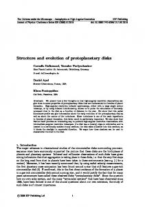
1SUPA, School of Physics and Astronomy, University of St Andrews, North .... the application of interferometry to observations of protoplanetary disks, this sec-.
EPJ Web of Conferences 102 , 0 0 00 9 (2015) DOI: 10.1051/epjconf/ 201 5 102 0 0 0 0 9 � C Owned by the authors, published by EDP Sciences, 2015
Interferometry and the study of protoplanetary disks� John D. Ilee1 and Jane S. Greaves1 1
SUPA, School of Physics and Astronomy, University of St Andrews, North Haugh, St Andrews, Scotland, KY16 9SS, UK
Abstract. Interferometry offers access to scales that are unresolvable using single dish telescopes, which is especially important when investigating objects with small angular sizes, such as protoplanetary disks. This Chapter introduces the concept of interferometry, and describes the basic aspects of interferometric observations when considering long (i.e. sub-millimetre to radio) wavelength observations. Examples of recent work using both continuum and spectral line observations are investigated, and their diagnostic power is examined. Finally, a selection of currently available facilities are=ussed, and the prospects of future instruments are explored.
1 The motivation for interferometry The use of interferometric techniques for the observation of astrophysical objects was first proposed in 1868 by Hippolyte Fizeau in order to measure the diameter of stars. Several years later, in 1891, Albert Michelson measured the size of the moons of Jupiter using the technique. However, it took until the construction of the Mount Wilson Observatory in California for Fizeau’s original idea to be realised, when the angular size of the photosphere of the massive star Betelgeuse was measured (Michelson & Pease 1921). Observing astronomical objects using interferometry offers several advantages over using single dish telescopes. The main advantage is one of spatial resolving power, and can be understood by way of a simple example. Consider the theoretical diffraction limit of a single dish telescope. For a D = 10 m class telescope operating at a wavelength of λ = 1 mm, we can use the Rayleigh criterion to define the highest angular resolution (limited only by diffraction) achievable for the telescope: θ = 1.22
λ ∼ 25 arcsec . D
(1)
Now, consider a young stellar system in a nearby star forming region that is located at a distance of 100 pc. Typically, circumstellar disks span several hundreds of astronomical units in radius (Andrews & Williams 2007; Dutrey et al. 1996). If the system is 100 au in diameter, it would subtend an angle of only 1 arcsec. The orbit of a Jupiter-like planet in such a system, located at a radial distance of approximately 10 au from the central star, would subtend an angle of 0.1 arcsec. In order to resolve such scales, a single dish telescope with a diameter of approximately 2.5 km would be required. This � 8th Lecture of the Summer School “Protoplanetary Disks: Theory and Modelling Meet Observations”
7KLV�LV�DQ�2SHQ�$FFHVV�DUWLFOH�GLVWULEXWHG�XQGHU�WKH�WHUPV�RI�WKH�&UHDWLYH�&RPPRQV�$WWULEXWLRQ�/LFHQVH������ZKLFK�SHUPLWV� XQUHVWULFWHG�XVH��GLVWULEXWLRQ��DQG�UHSURGXFWLRQ�LQ�DQ\�PHGLXP��SURYLGHG�WKH�RULJLQDO�ZRUN�LV�SURSHUO\�FLWHG��
Article available at http://www.epj-conferences.org or http://dx.doi.org/10.1051/epjconf/201510200009
EPJ Web of Conferences
is more than eight times larger than diameter of the world’s largest single aperture telescope at the Arecibo Observatory, and is clearly not feasible. Thus, in order to access smaller angular scales, the idea of a single telescope must be abandoned. Rather than using a single, large telescope to collect light, multiple smaller telescopes can be combined together in an array to simulate a larger telescope. Such a collection of smaller, linked telescopes is referred to as an interferometer. In these cases, the limiting factor for resolution is no longer the size of the individual telescopes (which determines the photon collecting area and the field of view), but rather the spacing between the telescopes - also known as the baseline length. To understand why this is the case, we can compare a simple two-telescope interferometer to the classic Young’s double slit experiment. If planar monochromatic wave fronts are passed through a screen with two slits, the resulting illumination pattern is composed of bright and dark bands - known as interference fringes - due to the constructive and destructive interference between the secondary waves emitted from the slits. Figure 1 shows a diagram of a simple Young’s double slit experiment, where an intensity distribution I of interference pattern is created.
I 1 0 1 0 1 0 1 0 1 0 1 0 1 0 1 0 1 0 1 0 1 0 1 0 1 0 1 0 1 0 1 0 1 0 1 0 1 0 1 0 1 0 1 0 1 0 1 0 1 0 1 0 1 0 1 0 1 0 1 0 1 0
θ
B
y
L Figure 1. Example of the Young’s slit experiment. Planar monochromatic wavefronts (not shown) passing through two slits separated by a distance B constructively and destructively interfere, producing alternating bright and dark bands on an observation screen. These bands are called interference fringes, and the constructive interference peaks are located at a linear distance y, or an angular distance θ, from the centre axis.
A constructive interference pattern is produced when the path difference between the two rays is an integer number of wavelengths (λ). If the separation between the slits (B) is much shorter than the distance to the detection screen (L), then the path difference can be written as B sin θ and the condition for a maximum is then given by B sin θ = mλ ,
(2)
where m is any real integer number. In the case that y � L, the path difference can be approximated to sin θ = y/L. The spatial coordinates of constructive interference on the screen, or the fringe spacing, is then given by y=
mλL , B
00009-p.2
(3)
Summer School „Protoplanetary Disks: Theory and Modeling Meet Observations‰
and thus the spacing between successive constructive interference fringes is δy = λL/B, or in angular spacing, λ θ∝ . (4) B If we imagine that instead of two slits in a screen, we now have two telescopes (or antennas, as we shall hereafter refer to them) forming a baseline pair, and receiving planar wavefronts from an astrophysical object, then a similar relationship applies. Constructive interference fringes represent the spacing at which the telescope signals can be combined together. The angular spacing, θ, of the fringes is analogous to the resolution that the baseline pair is sensitive to. Therefore, an increase in baseline B leads to a smaller resolvable angular scale θ, and thus the limiting factor that determines the angular resolution of an interferometer is not the size of the individual antenna, but rather the maximum baseline between the elements that make up the array. By using varied baseline lengths (e.g. multiple antennas forming many different baseline pairs of varied lengths in an interferometric array) we can obtain signals on a range of angular scales, and combine these signals to build up an image of the target. However, this approach does come at a cost. The antennas cannot be spaced closer than their physical size would allow - an issue referred to as the zero spacing problem. Using Eq. (4), it can be seen that a minimum value of B means that scales larger than the corresponding θ will not be observable, leading to what is known as ‘resolving out’ large scale structure. Consequently, in order to recover emission from the largest regions that are resolved out by the interferometer, supplementary observations are required. Often, observations using separate single dish telescopes are combined with interferometric observations to provide information across a large range of scales (e.g. the southern Galactic plane survey, McClure-Griffiths et al. 2001). At the Atacama Large Millimeter/submillimeter Array (ALMA), there are two additional components, the ALMA Compact Array (ACA) and the Total Power (TP) array, that can be used alongside the main array to ensure information from larger scales is not lost.
2 Basics of interferometry Before discussing the application of interferometry to observations of protoplanetary disks, this section will cover the main ideas and relationships behind the method of interferometry. We note that this is not intended to be a thorough derivation of the fundamentals of interferometry, but should provide a sound basis for the understanding of observations presented in further sections, and act as a first step for the discovery of more in depth reviews and textbooks (e.g. Glindemann 2011; Taylor et al. 1999; Thompson et al. 2008). We also note that we do not discuss aspects of short wavelength (i.e. infrared and optical) interferometry, and instead point interested readers to several comprehensive reviews on this subject (e.g. Jankov 2010, 2011; Malbet 2009; Monnier 2003; Monnier & Allen 2013) 2.1 The (u, v) plane
It is useful to define a reference frame upon which to build the majority of the relationships that govern the recovery of observables from the output of an interferometer. This reference frame is known as the (u, v) plane, and its relationship to the sky image plane is shown in Fig. 2. Consider a source under observation possessing a brightness distribution I, expressed on coordinates of right ascension (x) pointing East, and declination (y) pointing North. The vector w points directly to the centre of the observations from the first antenna. The vectors u and v are respectively the East–West and North–South components of the projected baseline of the interferometer onto the 00009-p.3
EPJ Web of Conferences y
Pole
I(x,y)
x
v
w
u
w’
v’
u’
Figure 2. The relationship between (u, v) space and the image domain (x, y). The y-direction is oriented towards North, and the w-direction is oriented towards the observational target. The circle at (u� , v� , w� ) represents a baseline between two antennas.
plane of the sky. The loci of this baseline are therefore located at (0, 0, 0) and (u� , v� , w� ) in what is known as the (u, v) plane. 2.2 The visibility domain
Observations using conventional telescopes directly measure the distribution of brightness across the target, I(x, y). However, observations using interferometers cannot directly measure this brightness distribution. Instead, interferometers measure the coherence of signals received at each antenna making up the array. This quantity is called the visibility, and can be understood by considering a simple analogy to the Young’s double slit experiment. For such an experiment, the visibility is given as V=
Imax − Imin , Imax + Imin
(5)
where I is the intensity of the interference pattern on the plane of observation. In a situation where a point-like source emits plane monochromatic waves at the optical axis of the double slit experiment, the signals from the two slits will be coherent, and alternating constructive and destructive interference patterns will be produced on a screen. This corresponds to a maximum intensity of one, and a minimum intensity of zero, giving V = 1 (Fig. 3, left). If, however, there are two point-like sources separated by half the angular separation of the constructive maxima, then two sets of such interference patterns will be cast on a screen out of phase with one another, cancelling each other out. In this case, the maximum intensity is equal to the minimum intensity, giving V = 0 (Fig. 3, right). If we consider a more complex source structure, then a useful simplification involves thinking of this structure as being made up of a series of point-like emitting sources. In such cases, also of 00009-p.4
Summer School „Protoplanetary Disks: Theory and Modeling Meet Observations‰
θ/
2
λ
φ
θ 1
1
I
I 0
0
V=1
V=0
Figure 3. Example of the visibilities for Young’s double slit experiment illuminated with plane, monochromatic waves from sources at infinity. Left: the intensity distribution for a single point source, with a visibility of one. Right: the intensity distribution for two sources separated by half the angular separation of the intensity peaks, with a visibility of zero. Based on Monnier (2003).
interest is the relative phase, φ, of the interference patterns produced by each region of the structure. As we can see from Fig. 3, this phase is related to the delay of the signals reaching each antenna, and it therefore gives information on the angular seperation, and thus spatial scale, of the object being observed. In the following, we will only consider the treatment of monochromatic wavefronts. The effects of polychromatic waves as a function of time, while important, is beyond the scope of this Chapter, but is thoroughly discussed in Taylor et al. (1999) and Thompson et al. (2008). In general, the visibility is usually expressed as a complex quantity in terms of the amplitude of the fringes, |V|, and phase difference, φ, of the components which make up the fringes, giving V = |V| e−i φ ,
(6)
which is known as the complex visibility. We can relate the visibility measured by the interferometer in telescope baseline co-ordinates (u, v), to the sky brightness distribution in (x, y) co-ordinates via the spatial coherence function, �� � � V(u, v) = I(x, y) e− 2π i ux + vy dx dy . (7) The spatial coherence function can be inverted by a Fourier transform to yield the intensity distribution of the source, �� � � I(x, y) = V(u, v) e 2π i ux + vy du dv , (8) a relationship known as the van Cittert-Zernike theorem (van Cittert 1934; Zernike 1938), which simply states that the output signal of an interferometer is a Fourier transform of the observed brightness distribution of a source on the sky. Often, the visibility amplitude can be used directly to understand simple source structure. It can be plotted against the √ (de-projected) baseline buv , which is given by the addition in quadrature of u and v such that buv = u2 + v2 . This produces a visibility curve, examples of which are shown for various brightness distributions in Fig. 4. 00009-p.5
EPJ Web of Conferences y
y
I(x,y)
y
I(x,y)
I(x,y)
x
x
V
x
V
V
buv
buv
buv
Figure 4. Visibility as a function of baseline for three examples of brightness distributions. Left: A uniform disk geometry produces a sinc-like function in visibility, due to the sharp edge of the disc. Middle: A Gaussian disk geometry produces a smoothly declining visibility curve. Right: A binary source produces a sinusoidal-like visibility curve.
2.3 Aperture synthesis
The recovery of an observable from interferometry depends on the inversion of the complex visibilities V(u, v) into a brightness distribution I(x, y). Ideally, we would envisage a case where the (u, v) plane is filled, and it therefore fully samples the intensity distribution of our observational target. However, when using an interferometer this is not true, because the instrument is constructed of individual antennas, forming (often) fixed baseline pairs. In this case, discrete samples of (u, v) space are actually recovered. If the array is constructed of N antennas, then the number of baselines in the array (Nb ) and therefore the number of (u, v) samples, is given by Nb = 12 N(N −1). A sparsely-sampled (u, v) plane can introduce artefacts in the final images obtained from interferometry. Therefore, increasing the number of (u, v) samples is important to ensure that the closest approximation to the true sky brightness is obtained. If an object is under observation for a number of hours, then the rotation of the Earth changes the orientation of the array with respect to the source, increasing the (u, v) coverage. The first description and use of this technique was performed in the late 1960s involving the first observations of pulsars, for which the 1974 Nobel Prize was awarded. To illustrate this technique, Fig. 5 shows two examples of (u, v) coverage obtained from the SubMillimeter Array (SMA) facility. The first example (left) shows the (u, v) coverage that is obtained after observing a source for approximately 5 minutes. The second example (right) shows the (u, v) coverage obtained using the same antenna configuration, but after observing the target for 14 hours. Each point corresponds to a single integration of 30 seconds, and over time these begin to trace smooth arcs in (u, v) space, as the array moves with respect to the target due to the rotation of the Earth. However, there are still gaps in the (u, v) coverage even with a longer observation time. In order to fill these gaps, the antenna configuration can be changed, allowing previously unsampled (u, v) space to be sampled. This technique is used in facilities such as the Jansky Very Large Array (JVLA), in 00009-p.6
Summer School „Protoplanetary Disks: Theory and Modeling Meet Observations‰
100
SMA − 0.1 hours
100 50 v (kλ)
v (kλ)
50 0 −50 −100 −100
SMA − 14 hours
0 −50
−50
0 u (kλ)
50
−100 −100
100
−50
0 u (kλ)
50
100
Figure 5. Examples of the (u, v) plane coverage for the Sub-Millimeter Array (SMA). Left: Example of a relatively sparsely sampled (u, v) plane, taken over approximately 5 minutes. Right: Example of a more complete (u, v) coverage, taken over 14 hours, due to the rotation of the Earth. Courtesy Luke Maud (Maud 2013)
which each of the antenna are located on one of three arms making up a Y-shape, and moved to one of four reconfigurable positions periodically, or at the Atacama Large Millimeter/sub-millimeter Array (ALMA), where the individual antenna are relocated to various base stations using manually operated transporter vehicles. Thus, the combination of both reconfigurable antenna positions and the rotation of the Earth are often used together to build up a more complete (u, v) coverage during interferometric observations. 2.4 Deconvolution
A well filled (u, v) plane is crucial for high fidelity imaging. While aperture synthesis can be used to recover more (u, v) space, the effect of an incompletely sampled visibility domain still presents issues in the recovery of information from the observations. In practice, the full (u, v) space can never be completely recovered, and what is actually recovered is known as the ‘dirty image’ I D , which by using the van Cittert-Zernike theorem can be described by I D (x, y) = FT −1 {S (u, v) × V(u, v)},
(9)
where the sampling function S (u, v) is a series of delta functions giving unity in the sampled regions of (u, v) space and zero elsewhere, and FT −1 indicates an inverse Fourier transform. Classical convolution theory tells us that the dirty image can be described as a convolution, such that I D (x, y) = b(x, y) ⊗ I(x, y),
(10)
where b(x, y) = FT −1 {S (u, v)}, and is known as the ‘dirty beam’, and is analogous to the point spread function of a conventional telescope. Thus, recovery of the true intensity distribution of the source, I(x, y), involves removing the contribution of the dirty beam b(x, y) from the dirty image I D (x, y), which from Eq. (10) we can see is a deconvolution problem. Several methods have been developed to deconvolve the dirty beam from the dirty image - a process often referred to as ‘CLEANing’ - including the Högbom algorithm (Högbom 1974) and the maximum entropy method (Skilling & Bryan 00009-p.7
EPJ Web of Conferences
1984). A full derivation of the various procedures, their benefits and their subtleties is beyond the scope of this Chapter, but a comprehensive discussion can be found in Cornwell et al. (1999) and Jackson (2008). Figure 6 shows a diagram with examples of the relationship between the sampling function S (u, v), dirty beam b(x, y), dirty image I D (x, y) and final cleaned image I(x, y) for observations using the Sub-Millimeter Array (SMA).
3 Interferometric observations of protoplanetary disks Protoplanetary disks are, in a relative sense, small objects when compared to other large extended structures such as molecular clouds. As such, they can often be encompassed within the field of view of an interferometer and only require a single pointing (rather than a mosaic of pointings). Disks do not often possess extended emission, and therefore their largest angular scale is usually quite small. Thus, the zero spacing problem mentioned previously does not adversely affect the observations, and the main advantage that interferometry offers for the study of protoplanetary disks is one of spatial resolving power. In this section we will discuss interferometry involving longer wavelengths (i.e. sub-millimetre to radio), and examples of their power to analyse protoplanetary disks. Long wavelength interferometry was the first to be developed, due to the relative ease of construction of the antenna, the ability to locate them to within fractions of the metre-scale wavelengths considered, and the ability of the electronics of the time to correlate the signals in useful timescales. While single dish optical imaging offers much higher spatial resolution than observations of an equivalentlysized telescope in the sub-millimetre regimes, there are many benefits to using longer wavelength observations, particularly when combined with interferometric techniques. When considering circumstellar disks, the high densities mean that optical observations are mainly tracing the surface layers of the disk. The central star is often very bright at these wavelengths, so very accurate subtraction or blocking with a coronograph is required. Furthermore, the light that is observed is not emitted directly, but is mostly scattered starlight, and thus a complete understanding of the scattering media is required for proper interpretation of the observations. The combination of long wavelength observations (which do not suffer from the above problems, but have an inherently lower resolution), with interferometry is very attractive, as it increases the spatial resolving power to comparable or better levels than in the optical. In this section, we will briefly outline possible uses for such observations. 3.1 Continuum observations
The sub-millimetre to radio region of the spectrum provides access to many important diagnostics of both the gas and dust content of protoplanetary disks. Dust continuum in the millimetre regime is usually optically thin, and therefore observations of this continuum efficiently trace the mass distribution of material in the disk towards the mid-plane, rather than the surface features that are traced with optical or infrared observations. Also, the stellar photosphere does not emit significantly at these wavelengths, and given that the disk emission is usually from large radii, such emission is easily disentangled. Additionally, observations in the centimetre regime provide information on the large-grain contribution to the total disk mass, and the slope of the sub-mm to cm spectral energy distribution (SED) can give information on the dust grain distribution and even the presence of pebble-sized objects in the disk. An example of interferometric continuum observations is given in Fig. 7. This shows dust continuum observations at 1 cm wavelengths of the pre-main-sequence star AS 209 taken with the Jansky Very Large Array (JVLA), which obtain sub-arcsecond resolution (∼ 0.2 arcseconds, Pérez et al. 00009-p.8
Summer School „Protoplanetary Disks: Theory and Modeling Meet Observations‰
FT−1 S(u,v)
100
+63d19’30’’
+19’00’’ Dec.
v (kλ)
50 0
+18’30’’
−50 −100 −100
b(x,y)
−50
0 u (kλ)
50
+18’00’’ 22h19m25s 20s
100
R. A.
15s
10s
Eqn. (9) V(u,v)
1.4
+63d19’30’’
ID(x,y)
1.0
+19’00’’ Dec.
Visibility
1.2
0.8 0.6
+18’30’’
0.4 0.2 0
20
40 60 80 Baseline (kλ)
+18’00’’ 22h19m25s 20s
100
R. A.
15s
10s
(u2 + v2)1/2
Eqn. (10) I(x,y)
+63d20’00’’
Dec.
+19’30’’ +19’00’’ +18’30’’ +18’00’’ 22h19m24s 21s
18s R. A.
15s
12s
Figure 6. Diagram depicting the relationship between the various quantities described in the previous sections, sampling function S (u, v), the dirty beam b(x, y), the visibilities V as a function of baseline (calculated as √ u2 + v2 ), the dirty image I D (x, y) and final cleaned image I(x, y). All panels are from Sub-Millimeter Array (SMA) observations of the massive young stellar object S140 IRS 1. Courtesy Luke Maud (Maud et al. 2013).
00009-p.9
EPJ Web of Conferences
Figure 7. VLA observations of the pre-main-sequence star AS 209, showing 1 cm dust continuum emission from the disk (colour scale), overlaid with the value of the spectral index α obtained within the 1 cm (Ka) band. The effective beam size is shown with the hatched ellipse. Pérez et al. (2012) discuss the more detailed spectral indices obtained by comparing several bands; here the errors in α range from 0.2 near the central star, up to approximately 1 at the fainter outer disk radii. (Courtesy Laura Pérez, Disks@EVLA Project, P.I. Claire Chandler)
2012). The high spatial resolution of the observations showed that at these long wavelengths, the disk emission is more compact than at shorter wavelengths, suggesting radial changes in the dust grain properties across the disk. The authors suggest that such features can be due to a radial dependence on the dust opacity. If such a dependence is caused by the growth of dust grains in the disk, then these observations show that the grains increase in size from micron-sized particles in the outer disk, to centimetre-sized particles in the inner disk. A possible explanation for such behaviour could be radial migration of the larger dust particles towards the central star. However, interpreting millimetre wavelength continuum observations presents several challenges, the main one being the unknown opacity of the dust grains. Estimates can be made based on the mass opacity, but are highly dependent on the assumed size distribution of grains (Draine 2006). The majority of mass in a circumstellar disk is in the gas phase, and a large fraction of the solid mass may be located in larger, unobserved particles or objects, which suggests mass estimates derived from millimetre continuum emission may actually be lower limits. 3.2 Spectral line observations
The millimetre wavelength regime also has many rotational transitions of small molecules that give a wealth of information on the gas dynamics and chemical processes occurring in circumstellar disks. Molecular hydrogen makes up the dominant source of gas mass in such disks, but transitions of this molecule are difficult to observe due to the lack of dipole moment, low transition probabilities and strong telluric absorption across the wavelength ranges of emission. In contrast, the next most 00009-p.10
Summer School „Protoplanetary Disks: Theory and Modeling Meet Observations‰
Figure 8. Channel maps of the CO J = 3–2 line observed towards the Herbig Ae star HD 163296 during ALMA science verification, exhibiting the closed loop structure expected from gas in Keplerian rotation. (See also de Gregorio-Monsalvo et al. 2013 and Rosenfeld et al. 2013).
abundant molecule, CO, with a relative fractional abundance of X(CO) ∼ 10−4 is easily observed at millimetre wavelengths, and can provide information on the morphology of the gas in the disk. A recent example of the diagnostic power of interferometric line data were the observations of the Herbig Ae star HD 163296 taken during ALMA science verification. The telescope observed the CO J = 3–2 line, which can be excited in the outer regions of the disk. Figure 8 shows the intensity of the J = 3–2 line centred on three velocity channels, corresponding to gas moving at 1.2, 0 and −1.2 km s−1 respectively. The channel maps show the closed loop structure that would be expected from such gas orbiting in a Keplerian disk around the central star. However, such was the spatial resolving power and sensitivity of the observations, a secondary loop structure is also visible, which has been attributed to the emission from the far side of the flared disk. Observations such as these allow a direct measurement of the scale height of the emission region in the disk, placing useful observational constraints on the geometry of protoplanetary disks, and the location of chemical species within them (de Gregorio-Monsalvo et al. 2013; Rosenfeld et al. 2013). Further transitions of other non-symmetric molecules with a dipole moment are also possible (for example, NH3 emits in the centimetre regime) and even more transitions are possible if the emitting molecule can invert, twist, or if the electrons within the molecule are able to change spin, see chapters by Dionatos (2015) and Kamp (2015). However, there are complications based on the information obtained about the gas in circumstellar disks from line observations. For example, high optical depths make some line fluxes largely insensitive to densities. Also, chemical processes affect the relative abundances of different molecules based on their location within the disk, and molecules may freezeout of the gas phase and be deposited in ices on the surfaces of dust grains in lower temperature regions, see chapter by Thi (2015).
4 Current facilties Over the past decades, there has been much investment in the development and commissioning of a new generation of long wavelength interferometric facilities, a selection of which are summarised in Table 1. In the radio regime, the upgrade of the Very Large Array to the Karl G. Janksy Very Large Array consisted of introducing state-of-the-art electronics to the facility. This increased the sensitivity of 00009-p.11
EPJ Web of Conferences Table 1. Examples of current and future long wavelength interferometric facilities.
Array
Location
Radio facilities LOFAR Europe JVLA USA WSRT The Netherlands GMRT India ATCA Australia e-MERLIN UK (Sub-)millimetre facilities KVN Korea ALMA Chile PdBI (NOEMA) France SMA USA
Antennas
Maximum baseline (km)
Frequencies (GHz)
50 × 35–85 m 27 × 25 m 14 × 25 m 30 × 45 m 6 × 22 m 7 × 25–76 m
2–1000 35 2.8 25 6 200
0.01–0.24 0.07–43 0.11–8.5 0.15–1.5 1.2–90 1.3–22
3 × 21 m 50 × 12 m 6(12) × 15 m 6 × 6m
476 16 0.76 0.5
22–129 30–850 80–371 180–700
the instrument by a factor of ten and reduced the finest frequency resolution by a factor of over 103 , bringing the instrument to the forefront of discovery in these wavelength ranges. The upgrade of the MERLIN network of seven radio telescopes in the United Kingdom to e-MERLIN provided an order of magnitude increase in sensitivity using new receiver technology. With baselines as long as 217 km, the inclusion of a dedicated optical fibre network connecting each telescope was essential to take advantage of a new correlator located at Jodrell Bank Observatory. When complete, the new facility will offer resolutions between 12–150 milliarcseconds in frequencies from 1.5–22 GHz. In the millimetre and sub-millimetre regime, the construction and commissioning of the Atacama Large Millimeter/sub-millimeter Array (ALMA) on Chajnantor plateau of the Chilean Andes is revolutionising the study of the southern sky. When completed, ALMA will offer baselines of up to 16 km and sensitivities a factor of 10–100 higher than other sub-millimetre interferometers. The upgrade of the Plateau de Bure Interferometer (PdBI) to the Northern Extended Millimetre Array (NOEMA) is scheduled to be completed in 2018, and will include doubling the number of antennas from 6 to 12, extending the longest baselines from 0.8 to 1.6 km, increasing sensitivity by almost a factor of 10, and providing a broad bandwidth of 32 GHz. The combination of ALMA and NOEMA will allow high resolution and high sensitivity access to both hemispheres in the sub-millimetre regime.
5 The future The study of protoplanetary disks is at an exciting stage, with a large amount of investment in new facilities from the radio down to the (sub-)millimetre regimes, allowing a huge range of wavelengths to be observed with unprecedented sensitivity and spatial resolution. The future holds even more impressive facilities - the completion of the Square Kilometre Array (SKA, see Fig. 9) in South Africa and Australia, currently scheduled for 2020, will provide a similar leap in capabilities that we have recently had across the sub-millimetre regimes. Observations at the long wavelengths offered by the SKA have the potential to directly discover how dust grains breach the so-called metre-scale barrier and grow into planetesimals. The SKA will also be uniquely placed to detect complex organic molecules in circumstellar disks. Recent models suggest that these complex organics exist in disks, but are below current sensitivity levels (Walsh et al. 2014). The recent detection 00009-p.12
Summer School „Protoplanetary Disks: Theory and Modeling Meet Observations‰
of a simple sugar, glycolaldehyde (HCOCH2 OH), around a solar-type star with ALMA has shown the possible wealth of chemical complexity that may exist toward young stars (Jørgensen et al. 2012). The detection of the smallest amino acid glycine (NH2 CH2 COOH) has so far only been confirmed in meteorites (Ehrenfreund et al. 2001) and comets (Elsila et al. 2009), while observations of hot cores have shown no detections (Snyder et al. 2005). Detection of this important pre-biotic molecule in the gas phase may be possible with the very high sensitivity of the SKA, and would push toward a more complete understanding of the formation of life on Earth.
Figure 9. Upper left: The proposed spiral antenna configuration of the Square Kilometre Array (SKA). Upper right: Artists impression of a protoplanetary disk, overlaid with a theoretical detection of complex organic molecules, which may be possible with the SKA. Bottom: Artists impression of the three different antenna types that will make up the array (courtesy SKA Organisation/Swinburne Astronomy Productions).
Acknowledgements We would like to thank Luke Maud for reading an early draft of this Chapter. We would also like to thank Laura Pérez and Luke Maud for kindly providing the data for several figures. The research leading to these results has received funding from the European Union Seventh Framework Programme FP7-2011 under grant agreement no 284405. This work makes use of the following ALMA data: ADS/JAO.ALMA#2011.0.00010.SV. ALMA is a partnership of ESO (representing its member states), NSF (USA) and NINS (Japan), together with NRC (Canada) and NSC and ASIAA (Taiwan), in cooperation with the Republic of Chile. The Joint ALMA Observatory is operated by ESO, AUI/NRAO and NAOJ. 00009-p.13
EPJ Web of Conferences
References Andrews, S. M. & Williams, J. P. 2007, ApJ, 659, 705 Cornwell, T., Braun, R., & Briggs, D. S. 1999, in Astronomical Society of the Pacific Conference Series, Vol. 180, Synthesis Imaging in Radio Astronomy II, ed. G. B. Taylor, C. L. Carilli, & R. A. Perley, 151 de Gregorio-Monsalvo, I., Ménard, F., Dent, W., et al. 2013, A&A, 557, A133 Dionatos, O. 2015, in EPJ Web of Conferences, Vol. 102, Summer School on Protoplanetary Disks: Theory and Modeling Meet Observations, ed. I. Kamp, P. Woitke, & J. D. Ilee Draine, B. T. 2006, ApJ, 636, 1114 Dutrey, A., Guilloteau, S., Duvert, G., et al. 1996, A&A, 309, 493 Ehrenfreund, P., Glavin, D. P., Botta, O., Cooper, G., & Bada, J. L. 2001, Proceedings of the National Academy of Science, 98, 2138 Elsila, J. E., Glavin, D. P., & Dworkin, J. P. 2009, Meteoritics and Planetary Science, 44, 1323 Glindemann, A. 2011, Principles of Stellar Interferometry (Astronomy and Astrophysics Library. ISBN 978-3-642-15027-2. Springer-Verlag Berlin Heidelberg) Högbom, J. A. 1974, A&A Suppl., 15, 417 Jackson, N. 2008, in Lecture Notes in Physics, Berlin Springer Verlag, Vol. 742, Jets from Young Stars II, ed. F. Bacciotti, L. Testi, & E. Whelan, 193 Jankov, S. 2010, Serbian Astronomical Journal, 181, 1 Jankov, S. 2011, Serbian Astronomical Journal, 183, 1 Jørgensen, J. K., Favre, C., Bisschop, S. E., et al. 2012, ApJL, 757, L4 Kamp, I. 2015, in EPJ Web of Conferences, Vol. 102, Summer School on Protoplanetary Disks: Theory and Modeling Meet Observations, ed. I. Kamp, P. Woitke, & J. D. Ilee Malbet, F. 2009, New Astron. Rev., 53, 285 Maud, L. T. 2013, PhD thesis, The University of Leeds Maud, L. T., Hoare, M. G., Gibb, A. G., Shepherd, D., & Indebetouw, R. 2013, MNRAS, 428, 609 McClure-Griffiths, N. M., Green, A. J., Dickey, J. M., et al. 2001, ApJ, 551, 394 Michelson, A. A. & Pease, F. G. 1921, ApJ, 53, 249 Monnier, J. D. 2003, Reports on Progress in Physics, 66, 789 Monnier, J. D. & Allen, R. J. 2013, Radio and Optical Interferometry: Basic Observing Techniques and Data Analysis (Springer Science+Business Media Dordrecht, ISBN 978-94-007-5617-5), 325 Pérez, L. M., Carpenter, J. M., Chandler, C. J., et al. 2012, ApJL, 760, L17 00009-p.14
Summer School „Protoplanetary Disks: Theory and Modeling Meet Observations‰
Rosenfeld, K. A., Andrews, S. M., Hughes, A. M., Wilner, D. J., & Qi, C. 2013, ApJ, 774, 16 Skilling, J. & Bryan, R. K. 1984, MNRAS, 211, 111 Snyder, L. E., Lovas, F. J., Hollis, J. M., et al. 2005, ApJ, 619, 914 Taylor, G. B., Carilli, C. L., & Perley, R. A., eds. 1999, Astronomical Society of the Pacific Conference Series, Vol. 180, Synthesis Imaging in Radio Astronomy II Thi, W.-F. 2015, in EPJ Web of Conferences, Vol. 102, Summer School on Protoplanetary Disks: Theory and Modeling Meet Observations, ed. I. Kamp, P. Woitke, & J. D. Ilee Thompson, A. R., Moran, J. M., & Swenson, Jr., G. W. 2008, Interferometry and Synthesis in Radio Astronomy, 2nd Edition (James M. Moran, and George W. Swenson, Jr., Wiley, ISBN: 978-0-47125492-8), 692 van Cittert, P. H. 1934, Physica, 1, 201 Walsh, C., Millar, T. J., Nomura, H., et al. 2014, A&A, 563, A33 Zernike, F. 1938, Physica, 5, 785
00009-p.15