Dec 5, 2014 - was initiated to decide if lowered fieldwork would produce acceptable .... (BHNF) with land management directed by the USFS (Figure 2).
Evaluasi dan Analisa Interpolasi Sistem Prediksi Hujan berbasis GIS menggunakan ArcGIS. 1Joe Yuan Mambu. Program Studi Sistem Informasi, Universitas ...
tested in assessing of site specific P variability on the apple ... nutrient requirements in order to plan a site-specific fer- ..... Predict soil texture distributions us-.
May 5, 2009 - Alfred Wegener Institute for Polar and Marine Research,. Potsdam ...... Wilson S, Hassell D, Hein D, Jones R, Taylor R (2005) Installing.
Jan 31, 2016 - The study was conducted in Medinipur block of Paschim Medinipur district ... Reconnaissance soil survey of Medinipur Block was carried out on ...
RANKING SPATIAL INTERPOLATION TECHNIQUES. USING A .... many other statistics in a report format. ... Another choice given in the software for coding.
Oct 8, 2006 - Key words: GIS, education, graduate and postgraduate course. .... domains of Geodesy, Geography or Computer Science. ..... form, Study characteristics, Coding format and instructions for coders, Pilot testing and form.
educational requirements for licensing and is recommended for prospective real estate salespersons who desire either a f
characterizations of interpolation spaces and their relations to a number of results in ..... the degree of P is odd, P(ât) is negative for large values of t, and so P(âαn) < 0 ..... vectors x(2), y(2) via (2.18) and (2.19) we will have Tx(2) =
The data used for the movies are simulated by Dr. Ying-Hwa Kuo form The National Center for. Atmospheric Research (NCAR) in Boulder, Colorado. We want to ...
Jul 3, 1998 - we want to construct a function interpolating these data. ... If we want a smooth e.g. Lipschitz interpolant of points and curves, the most invariant ..... the above definition, if it defines uniquely u, immediately implies the stabilit
general electrical system diagnosis, battery diagnosis and repair, starting system
... identify the ISO symbols used on hydraulic schematics and to trace the ...
and 73.41-75.37Ë E. This study evaluates the potential hydropower dam sites with huge discharges and documents the sensitivity .... study for small to large dam as Neelum-Jhelum hydropower ... basin by merging all order values in ARCGIS.
An indistinct design was shown to be an incised ... Along with a Canon Rebel camera, Adobe Photoshop software, and a ...
Along with a Canon Rebel camera, Adobe Photoshop software, and a program written by ... The field version of the RTI tec
Editora UFPR. Using Geographic Information Systems in science classrooms. Usando o Sistema de Informação. Geográfica (GIS) em salas de aula de ciências.
Sep 27, 2012 - Available online: http://www.unisdr.org/files/657_lwr21.pdf (accessed .... earth-conference2008/papers/papers/ A06ID092.pdf (accessed on 21 ...
Sep 27, 2012 - LANDSAT, ASTER and Google Earth data, in addition to available open-source data such as open-street-map ... ASTER- mission can contain horizontal and vertical errors up to several meters. ... providing information of highest surface wa
An indistinct design was shown to be an incised ... Along with a Canon Rebel camera, Adobe Photoshop software, and a ...
AbstractâPrediction of spatial attributes has attracted signif- icant research interest in recent ... some predicted value using interpolation. Moreover, the sensors.
The Wisconsin, Iowa, ..... (1996); DeWitt and Ralston (1996); and Docherty et al (1997a, 1997b). .... DeWitt W J, Ralston B A 1996 GIS: existing and potential.
All GST courses can be used to satisfy graduation requirements as general
elective credit. ... College Study Strategies (GST 116) - 3 credit hours/letter grade.
Cluster Sampling. Cluster centers are established. (random or systematic). Samples arranged around each center. Plot on map. Visit sample. (e.g. US Forest ...
INTERPOLATION Procedure to predict values of attributes at unsampled points Why? Can’t measure all locations: Time Money Impossible (physical- legal) Changing cell size Missing/unsuitable data Past date (eg. temperature)
Systematic sampling pattern Easy Samples spaced uniformly at fixed X, Y intervals Parallel lines
Advantages Easy to understand
Disadvantages All receive same attention Difficult to stay on lines May be biases
Random Sampling Select point based on random number process Plot on map Visit sample
Advantages Less biased (unlikely to match pattern in landscape)
Disadvantages Does nothing to distribute samples in areas of high Difficult to explain, location of points may be a problem
Cluster Sampling Cluster centers are established (random or systematic)
Samples arranged around each center Plot on map Visit sample (e.g. US Forest Service, Forest Inventory Analysis (FIA) Clusters located at random then systematic pattern of samples at that location)
Advantages Reduced travel time
Adaptive sampling
More sampling where there is more variability. Need prior knowledge of variability, e.g. two stage sampling
Advantages More efficient, homogeneous areas have few samples, better representation of variable areas.
Disadvantages Need prior information on variability through space
INTERPOLATION Many methods - All combine information about the sample coordinates with the magnitude of the measurement variable to estimate the variable of interest at the unmeasured location Methods differ in weighting and number of observations used Different methods produce different results No single method has been shown to be more accurate in every application Accuracy is judged by withheld sample points
INTERPOLATION Outputs typically:
Raster surface •Values are measured at a set of sample points •Raster layer boundaries and cell dimensions established •Interpolation method estimate the value for the center of each unmeasured grid cell Contour Lines Iterative process •From the sample points estimate points of a value Connect these points to form a line •Estimate the next value, creating another line with the restriction that lines of different values do not cross.
Example Base
Elevation contours
Sampled locations and values
INTERPOLATION 1st Method - Thiessen Polygon Assigns interpolated value equal to the value found at the nearest sample location Conceptually simplest method
Only one point used (nearest) Often called nearest sample or nearest neighbor
INTERPOLATION Thiessen Polygon Advantage: Ease of application Accuracy depends largely on sampling density Boundaries often odd shaped as transitions between polygons are often abrupt Continuous variables often not well represented
Thiessen Polygon Draw lines connecting the points to their nearest neighbors. Find the bisectors of each line. Connect the bisectors of the lines and assign the resulting polygon the value of the center point
1. Draw lines connecting the points to their nearest neighbors.
2
5 4
2. Find the bisectors of each line.
3. Connect the bisectors of the lines and assign the resulting polygon the value of the center point
2)
3)
Sampled locations and values
Thiessen polygons
INTERPOLATION Fixed-Radius – Local Averaging
More complex than nearest sample Cell values estimated based on the average of nearby samples Samples used depend on search radius (any sample found inside the circle is used in average, outside ignored)
•Specify output raster grid •Fixed-radius circle is centered over a raster cell Circle radius typically equals several raster cell widths (causes neighboring cell values to be similar)
Several sample points used Some circles many contain no points Search radius important; too large may smooth the data too much
INTERPOLATION Fixed-Radius – Local Averaging
INTERPOLATION Fixed-Radius – Local Averaging
INTERPOLATION Fixed-Radius – Local Averaging
INTERPOLATION Inverse Distance Weighted (IDW) Estimates the values at unknown points using the distance and values to nearby know points (IDW reduces the contribution of a known point to the interpolated value)
Weight of each sample point is an inverse proportion to the distance. The further away the point, the less the weight in helping define the unsampled location
INTERPOLATION Inverse Distance Weighted (IDW)
Zi is value of known point
Dij is distance to known point Zj is the unknown point n is a user selected exponent
•Size of exponent, n affects the shape of the surface larger n means the closer points are more influential •A larger number of sample points results in a smoother surface
INTERPOLATION Inverse Distance Weighted (IDW)
INTERPOLATION Inverse Distance Weighted (IDW)
INTERPOLATION Trend Surface Interpolation Fitting a statistical model, a trend surface, through the measured points. (typically polynomial)
Where Z is the value at any point x Where ais are coefficients estimated in a regression model
INTERPOLATION Trend Surface Interpolation
INTERPOLATION Splines Name derived from the drafting tool, a flexible ruler, that helps create smooth curves through several points Spline functions are use to interpolate along a smooth curve.
Force a smooth line to pass through a desired set of points Constructed from a set of joined polynomial functions
INTERPOLATION : Splines
INTERPOLATION Kriging Similar to Inverse Distance Weighting (IDW) Kriging uses the minimum variance method to calculate the weights rather than applying an arbitrary or less precise weighting scheme
Interpolation Kriging Method relies on spatial autocorrelation Higher autocorrelations, points near each other are alike.
INTERPOLATION Kriging A statistical based estimator of spatial variables
Creates a mathematical model which is used to estimate values across the surface
Kriging - Lag distance
Zi is a variable at a sample point hi is the distance between sample points Every set of pairs Zi,Zj defines a distance hij, and is different by the amount Zi – Zj. The distance hij is the lag distance between point i and j. There is a subset of points in a sample set that are a given lag distance apart
Kriging - Lag distance
INTERPOLATION Kriging Semi-variance Where Zi is the measured variable at one point Zj is another at h distance away n is the number of pairs that are approximately h distance apart Semi-variance may be calculated for any h When nearby points are similar (Zi-Zj) is small so the semivariance is small. High spatial autocorrelation means points near each other have similar Z values
INTERPOLATION Kriging When calculating the semi-variance of a particular h often a tolerance is used Plot the semi-variance of a range of lag distances This is a variogram
INTERPOLATION Kriging When calculating the semi-variance of a particular h often a tolerance is used Plot the semi-variance of a range of lag distances This is a variogram
Idealized Variogram
INTERPOLATION (cont.) Kriging •A set of sample points are used to estimate the shape of the variogram •Variogram model is made (A line is fit through the set of semi-variance points) •The Variogram model is then used to interpolate the entire surface
Class Vote: Which method works best for this example? Systematic
Random
Original Surface:
Cluster
Adaptive
Class Vote: Which method works best for this example? Thiessen Polygons
Fixed-radius – Local Averaging
IDW: squared, 12 nearest points
Original Surface:
Trend Surface
Spline
Kriging
Interpolation in ArcGIS: Spatial Analyst
Interpolation in ArcGIS: Geostatistical Analyst
Validation
Interpolation in ArcGIS: arcscripts.esri.com
What is the Core Area?
Core Area Identification • Commonly used when we have observations on a set of objects, want to identify regions of high density • Crime, wildlife, pollutant detection • Derive regions (territories) or density fields (rasters) from set of sampling points.
Mean Circle
Concave Hull
Convex Hull
Kernal Mapping
Smooth “density function” One centered on each observation point
Sum these density functions
Sum the total, for a smooth density curve (or surface)
How much area should each sample cover (called bandwidth)
Varying bandwidths a)Medium b)Low h c)High h d through f are 90% density regions