IASE/ISI Satellite, 2003: Rolf Biehler
Interrelated learning and working environments for supporting the use of computer tools in introductory classes Rolf Biehler University of Kassel, Dept. of Mathematics/Informatics, Heinrich-Plett-Str. 40, 34130 Kassel, Germany
[email protected] At the department of mathematics & informatics in our University we are in the process of redesigning our introductory course on stochastics (probability and statistics) for future mathematics teachers. In this course we now use the software FATHOM, which students learn as a (cognitive and culturally mediated) tool for exploratory data analysis, for simulation and for inferential statistics as well as a tool for experimenting with statistical methods. We use various types of Internet based materials to support the learning process of our students. Experimental learning environments and working environments containing data and exploratory guides are constructed with FATHOM. FATHOM offers meta-medium and meta-tool capabilities that offer high adaptability and versatility for the teacher of a course. In addition, we have developed Java applets, screen videos and web-based hypertexts as further supporting materials. 1. Introduction The course we will describe is called “Elementary Stochastics”. It is obligatory at our department for all student teachers for grade 5 to 10 (pupils aged 11 to 16 years). Stochastics is the name for probability and statistics in the German school system. The course content is concerned with stochastics as a subject matter and not directly concerned with the didactics of stochastics, which is the topic of other courses. Stochastics is part of most syllabi and school textbooks in Germany but teachers often skip stochastics if they get under time pressure at the end of the school year. This is partly due to fact that teachers have not studied stochastics during their pre-service education at university. More and more universities have now included obligatory stochastics courses for their student teachers, but often these courses do not integrate work with computers and with real data so that the type of stochastics learned does not well prepare them for teaching stochastics from an innovative point of view, that is using real data and simulations, using authentic problems and using computers as cognitive tools. The course we are developing is to fill this gap. We are experimenting with new course content, working style and course materials in Kassel as a first step of further development and publication. In this sense, I am reporting about ongoing work. We have taught this course two times so far, in the winter semester 2001/02 and 2002/03. We, this is Klaus Kombrink, who is responsible for the laboratory work, several student teaching assistants and myself. The course has about 45 hours for lecturing and about 30 hours laboratory and practice sessions. For assessment, students are required to weekly work on a set of tasks and submit their solutions. In addition, there is a written examination at the end and the need to do a statistical project and submit a “project report”. The course has new content emphasis: descriptive statistics is extended to exploratory data analysis, probability includes computer simulation from the beginning, and we include basic ideas concerning confidence intervals, hypothesis testing and fitting functions to data. Throughout the course, we use real data. In agreement with David Moore (1997) we think that we can exploit the synergy between new content and new pedagogy. The laboratory sessions are more devoted to exploratory learning with computers than they used to be and we intend to stimulate and support elements of statistical thinking by cognitive apprenticeship. Several students do their Ph.D. or Master thesis in relation to the course development and study the
IASE/ISI Satellite, 2003: Rolf Biehler
development of students’ competence in our course. Preliminary results of this accompanying research will be reported elsewhere. Computer, Internet and media use in the course will be described in more detail later. We start with some general considerations. Some years ago, I developed the view that what we need most for introductory courses is a tool that can support both the learning and the doing of statistics (Biehler, 1993, 1997). Such a software tool should fulfill a lot of criteria in order that it can serve as a tool for exploring data, a tool for elementary simulations, a tool for studying mathematical functions and sequences that are relevant in stochastics and at the same time serve as a meta-tool and meta-medium by which teachers and learners can construct and adapt learning and working environments for teaching and learning purposes, especially for defining adequate visualizations and experimental environments (micro worlds). Since a few years, software is available that nearly perfectly fits these requirements, namely the software FATHOM. We are using FATHOM for a multiplicity of purposes in our course and are still exploring the potential and the limits of this software. Basically, we use FATHOM as a tool. Above that, we provide prepared FATHOM worksheets with visualizations or with experimental environments. FATHOM produces graphs and numerical results. Furthermore one can add text and graphs to a FATHOM worksheet. By these means analysis results can be annotated. Annotation can be comments, interpretations or in the case of working environments contain tasks or exploration guidelines. We use this feature to show exemplary students’ work or exemplary “expert work” concerning data analyses or simulations that we consider as prototypes that can orient students’ work. These resources together with real data sets are provided via the intranet. In addition to FATHOM based material we have dynamic slide shows and screen videos that are useful for two purposes: Showing more difficult uses of the software in a dynamic way and showing prototypical data analyses as a process with self-reflecting components. We use the metaphor of “thinking aloud” to design these screen videos and slight shows. A “hyperscript” will replace conventional lecture notes. The limited space of this paper will be used to provide an inside into our work by showing some experimental environments, by presenting elements of our module exploring data with a focus on comparing several distributions. We will finish with providing a short glance into how we deal with the topic of simulation and modeling. 2. Constructing experimental environments A standard applet on many Internet pages and multimedia material is concerned with showing how the mean and the median behave differently when one changes individual data points or outliers. Usually, an artificially chosen data set will be visualized in some standard form as by a histogram or dot plot, the mean and median will be shown in the graph and the user can change data values and observe the result. Sometimes, changing a data value can automatically happen so that a short movie, a dynamical graph can be observed. I will use this example for showing basic building blocks of FATHOM. The environment of the screen picture in Fig. 1 can quickly be constructed. We define an empty collection, add a variable var and enter 6 cases with the values shown. We insert a slider a and define var1 by the formula var + a . The variable var1 just contains the same values as the variable var if (caseindex = 1) var except in the first row, where we are adding the number a, which has the value 7 in Fig. 1. We have produced dot plots of var and of var1. We have enriched both displays by the command plot value and plotted the mean( ) and median( ) values of the respective variables. If we do not insert an attribute into the function mean( ) the actual attribute of the display will be used (so if we change the attribute in the display the mean of the new attribute will automatically be calculated).
IASE/ISI Satellite, 2003: Rolf Biehler
Fig. 1 Exploring median and mean (Screen picture from FATHOM)
Using the prepared environment. We can change the slider a by moving the slider or we can give the slider a push so that the variable a automatically changes between the boundaries of the slider. The change results in a change of the first line of var1 in the collection, which results in the change of the data point in the lower display, and a change of mean (var1), which effects the line of the mean in the lower display. Multiple dynamically linked windows are the basis for the propagation of changes. Modifying the prepared environment. As compared to Java applets, a major advantage of FATHOM worksheets is that teachers and learners can easily modify the worksheet themselves, for instance: other distribution displays than the dot plot can be chosen from the graph menu, (such as the percentile plot or the histogram), the formulas for the plot value command can be replaced by a different one so that other statistically defined values can be added to the plot, other data can be used: it is just necessary to copy another variables’ values in the first column of the table. This option is a fundamental advantage because one can use one’s own data for the experiment. This simple environment illustrates the meta-medium facilities of FATHOM, which can be can be used to construct even more complex experiments.
Fig. 2 Exploring normal and binomial distributions (Screen shot from FATHOM)
IASE/ISI Satellite, 2003: Rolf Biehler
The screen picture of Fig. 2 shows an environment that allows changing parameters of the binomial and normal distribution and fitting the latter to the first. A display with empty data was used, by which FATHOM is transformed into a function plotter. Again, one can easily modify the environment: instead of controlling the parameters of the normal density curve by sliders in order to explore which parameters fit best, we could change the formula to normalDensity(x, np, sqrt(np(1-p))). Changing n and p will now show how well the normal curve approximates the binomial when using the mean and the standard deviation of the binomial as parameters for the normal. The aim of this visualization is different from the aim of the first one. The instructor can easily fine-tune visualizations according to his/her needs. Let me remark that the screen picture do not show another important feature of FATHOM we use, namely the possibility to add text windows into the worksheet at all places where it is needed. Text may contain comments, or tasks, or guidelines for exploration. 3. Exploring data 3.1 Studying variation, comparing distributions
Traditionally descriptive statistics is concerned with univariate distributions and their graphical and numerical summaries. Histograms, bar charts, box plots, measures of location and spread are introduced and used. Descriptive statistics is an entrance level of dealing with variation. Wild & Pfannkuch (1999) identify the consideration of variation as one of the central components of statistical thinking. They distinguish different important statistical activities or goals concerning variation: noticing, acknowledging, explaining, dealing with, measuring and modeling for prediction, explanation and control. I like to explicitly add describing and summarizing. Changing representations for discovery & communication is named transnumeration by Wild & Pfannkuch. It is also relevant here in that one display or summary is not enough for studying a distribution. A box plot, for instance, provides a certain view or model of the data and in general it is useful to use other displays and summaries as well when one studies the distribution of a variable. FATHOM supports transnumeration skills because various displays are “at hand” and can be compared. Its feature of multiple linked representations and of enriching graphs can help to relate information across graphs. We discuss several examples for illustrating Fathom’s capabilities, our didactical approach and the data and environments that we use. Fig. 3 shows the weekly hours about 540 students purposefully spend on TV according to their own estimates. This is one of the variables of the MUFFINS data set (see below). I have enhanced the dot plot with median and quartiles. The menu in the northeast corner has options for all the other relevant displays. The arrangement of windows supports display comparison: Students are to see the same information in both graphs as well as what can be seen in one of the graphs only. In this case the dot plot shows popular values at multiples of 5 hours and of 7 hours, which are not visible in the box plot. The contextual reason is how students have estimated (x hours per day times 7 or just multiples of easy numbers (5)). Integrating the statistical and the contextual is another important aspect of statistical thinking that is relevant here. Whereas traditional descriptive statistics was often concerned with just summarizing or displaying distributions, exploratory data analysis in our understanding (Biehler,1994a) seeks to relate distributions to their contexts, to the process or processes that have generated the data (see also Konold & Pollatsek, 2002). The tasks and examples we are using should encourage this way of thinking. In an elementary way students may ask whether extraordinary circumstances explain the outliers of more than 30 hours (the persons belonging to the outliers can be identified with the software and their behavior can be studied).
IASE/ISI Satellite, 2003: Rolf Biehler
Fig. 3 Comparing Boxplot and Dotplot (Screenshot from FATHOM)
Related to this contextual approach, we intend to go beyond traditional aims of descriptive statistics in the direction of including “group comparison” tasks and developing students’ strategies for group comparison. In the above example one may ask how the availability of a TV set in the student’s room at home may “effect” the time spent at the TV. Fig. 4 shows box plots for the two groups that exhibit quite a difference. Box Plot
OwnTV_set no yes
Muffins
0
5
10
15
20
25
30
35
Time_TV
Fig. 4 Time spent on TV grouped by OwnTV_set (yes,no)
The software FATHOM supports quick group comparisons. We just drag the attribute OwnTV_set to the y-axis of the box plot of Fig. 3 and get the box plot in Fig. 4. The northeast menu can be used to easily change the type of display. This makes it easy to explore whether we can find further differences in addition to those the box plots are already showing. Students’ competence has to be developed on three different levels: understanding the information in one graph (such as Fig. 4), relating this information in other graphs and judging the contribution of the various graphs to an overall comparison, and relating the information to the context. In this case the latter requires a sensible interpretation with regard
IASE/ISI Satellite, 2003: Rolf Biehler
to attributing causal relations: the availability of a TV set can influence the time of use, and vice versa, the intended time of use can influence whether someone has a TV-set in his/her room. Relating information to the context was required earlier already: When thinking about the distribution in Fig. 3 one must have the context-related “idea” of considering OwnTV_set as a potentially influencing factor. In this case, the first level (understanding the information in one graph) requires among others to recognize the shift of the box, the change in the spread (interquartile range) and the fact that the minimum 0 is the same in both groups. This may raise a further question Muffins Summary Table about the number of students that spend zero time on TV in Time_TV both groups. This is an information that can be better seen 172 no in dot plots. Alternatively, we can use a summary table 8 OwnTV_set (Fig. 5). The summaries in the table can be selectively and 357 yes adaptively defined in FATHOM. In sum FATHOM does make 3 nearly everything easy in a technical sense, but students Column Summary 529 have to be enabled to make statistical and subject matter 11 related use of this potential. S1 = count ( ) S2 = count (?, Time_TV = 0)
Fig. 5
In the practice of the course, students are required to write reports on their analysis. Technically they have to enhance FATHOM worksheets with text and to arrange the graphs and summary tables in a sensible order, or they can copy every graph and table to a word processor for writing up the report. The organization of the laboratory sessions and the feedback students receive for their written work are directed towards apprenticeship learning of statistical thinking. In the ongoing developmental step of our project however we are developing further material for supporting this type of thinking. Prototypical interpretations of single graphs, of relating different graphs and of integrating the contextual will be provided by means of prototypical products that should exhibit different levels of successfully interpreting data. We will use products from students of the previous generation and make them available on the Internet in order to stimulate peer learning beyond the synchronic cooperative learning in the laboratory sessions. Slide shows and screen videos will be to illustrate the process of data analysis. We have been using programs such as CAMTASIA for producing screen videos and VIEWLET BUILDER for producing applets with slide shows. Group comparison tasks require transnumeration skills, the integration of the statistical and the contextual, and students have to deal with variation in a problem oriented way. The group comparison tasks we require from our students have proven to be much more difficult than expected, because students have to develop concepts and criteria for comparison that are not “natural” to them. For instance, look at the following questions “Do female students do more home work than male ones?” and “How do male and female students differ with regard to amount and type of computer use?” These are typical questions we raise and that our students have to refine so that they can be explored in a statistical sense. Given that there is a lot of variation in each group what at all do we mean when we ask “Do TV owners watch more TV than those who do not have a TV?” There are different explications of this question: we can use means or medians for comparison or we just compare the percentages that are below a certain limit. Sometimes all criteria point into the same direction, sometimes not, so that there is not a clear answer. Also other features as just a shift to higher values of the whole distribution can occur, such as an increase in spread. We can use again FATHOM for designing small environments to support conceptual development that seems to be difficult (Biehler, 1997a)..
IASE/ISI Satellite, 2003: Rolf Biehler
Fig. 6 Comparing distributions using limit points
The environment in Fig. 6 draws a cutoff point at c (=10). The value of the slider c can be changed. The summary table shows the relative proportion of students in each group who’s Time_TV is less than the value c. The proportion is higher or equal in the no group for all values of c. This is another criterion for saying that TV owners. It can be reasonable to pick out some other interesting values of c Moreover one should not only state that the proportion in the no-group is higher but also report how much higher it is. The formula we use in the summary table to calculate the relevant proportion is a bit complex because the command proportion refers to the whole data set but we want the proportion relative to the respective group. A partly simpler environment is the following. We select all students with Time_TV less then 10 hours. This selection is highlighted in the ribbonchart in the right part of Fig. 7, showing that the relative proportion in the no group is higher than in the yes group (the height of the red area is proportional to this proportion, the area is proportional to the fraction as part of the whole group.
Fig. 7 Comparing distributions with a limit point: Linked displays 3.2 Data, tasks and software support
The variables we used in the preceding paragraph are part of the complex MUFFINS data that we have collected set that students can use for exploring questions that we discussed. The
IASE/ISI Satellite, 2003: Rolf Biehler
multivariate nature is needed so that hypotheses and indications that have been raised in one step of analysis can be further explored in the next step. The multivariate nature is the basis for integrating the statistical and the contextual. One of the data sets we use in our course is the MUFFINS data (Biehler, Kombrink, & Schweynoch 2003). We designed a questionnaire for assessing how school students use their spare time and how and how long they use Internet, computer and other media in their everyday life. I will refer later to the original data of 540 students of grade 11 that we collected in the year 2000. The questionnaire and the data set can be downloaded from the Internet (http://www.mathematik.uni-kassel.de/didaktik/MUFFINS). An on-line version of the questionnaire is also available. Schools and courses that subscribe to the MUFFINS project can use this facility to collect data from their own students and extend the available data set. Thus the advantage of students analyzing their own data is combined with the advantage of having a larger data set that allows more interesting comparisons. In this sense we are about to build up a data-sharing project in the sense of Feldman et al. (2000). The data set contains ordinal variables on how often students do selected activities (6 categories from seldom to daily), for instance going out with friends for eating and drinking, hanging around, sports, art and music etc. In a next step students have to indicate at which time they get up in the morning, when they go to bed and when they are at school. This information is used to calculate every student’s time budget in a week. We subtract a global amount of 15 hours per week for meals and personal hygiene. The resulting time is the net time budget (in weekly hours). Within this budget students have to estimate how many weekly hours they spend purposefully for 9 activities: using the TV, listening to music, using a computer, reading, doing music, doing sports, doing home work, helping in the household, jobbing. Further questions are related to how they use different facilities (TV for games, computer for internet etc.). Furthermore, their interest in various different types of telecasts, their use of and interest in newspapers, the kind of active or passive sport that interests them, are contents of other questions. We use the data for three didactical functions in our course: examples for introduction of new methods and displays, mini-applications, or “discovery journeys”. The group comparison tasks we have showed above are best described as mini-applications. Tasks for discovery journeys are for example (1) Jobs: How many have a job? In which domain? How much do they earn? How do the earnings depend on sex and domain? (2) Computer and Internet: How much time? How frequent? Which purpose? Dependent on which factors? (Sex, availability) (3) How different is the net time budget, what are factors influencing the net time budget? The latter topic can also be used for introducing bivariate methods. In early stages of teaching linear regression, we ask students to eye-fit linear functions to a scatter plot and control the fit by residual plots. An obvious hypothesis is that sleeping time has an effect on net time budget. The functional relation is also clear: if the average weekly sleeping time increases by one hour per week, we expect to gain additional 7 hours in our net time budget. We expect that a function Net_timebudget = 7 * mean_sleeping_time + a could fit the data. Deviations from this model can be due to other factors such as time at school and travel time to school. In a discovery journey context, students will have to calculate mean sleeping time from the other variables, decide about method of fitting etc. In an introduction context, the teacher can prepare the following system of windows in Fig. 8. The dot plot and the scatter plot are arranged one beside the other: whereas the dot plot shows the variation “as such” the scatter plot includes a variable “partly explaining the variation”. FATHOM supports plotting all mathematical functions into the scatter plot that can be defined with its formula editor. In this case we have made the function dependent on a slider a. The southeast plot is a residual plot, which is dynamically dependent on the data and the chosen function: If we move a, then the function graph and the residuals change dynamically. The learner has now to choose an adequate a, and teachers can raise the question of criteria of adequacy. Intuitively s/he might aim at residuals whose median is zero. In our Fig. 8 I have done my best to get the line
IASE/ISI Satellite, 2003: Rolf Biehler
through the middle of the points. Nevertheless, the residuals show a trend. Obviously the slope of –7 is not adequate to completely eliminate the trend. We have to stop our discovery journey here. The example was shown to illustrate again FATHOM as a meta-medium for designing learning environments. We can also use these displays as part of screen videos and applets that demonstrate prototypical data analyses with reflective “loud thinking” as we pointed out at the beginning.
Fig. 8 An experimental environment for fitting functions to data 4. Simulation and modeling
Fig. 9 Three stochastically independent dice A second important component of our course is simulation and modeling, which can be very briefly described only because of limits of space. We assume that students know FATHOM as a data analysis tool and that they can use this competence for analyzing simulated data. Simulation is integrated in the development of probability from the beginning. When we
IASE/ISI Satellite, 2003: Rolf Biehler
introduce probability for events E, we discuss counting the elements of the set E (combinatorial methods) for determining a probability in parallel to estimating the probability of E by simulation. Random variables will be informally introduced relatively early, shortly after having introduced the notion of random experiment and the notion of sample space. The screen picture of Fig. 9 shows an environment where three dice (equally distributed outcomes) are defined together with an event E and two random variables X1 and X2. Technically this is realized by “transformed variables”, conceptually students can build on the notion of a statistical variable. The distribution of the “variable” E is shown the bar graph, for X1 we see the histogram with inserted mean (which according to theory is approaching 3*3.5=10.5). We have used 1500 repetitions: each line represents a repetition. Such environments can be prepared and given to the students for explorations (they may add further events or random variables of interest) or students are asked to construct such environments themselves. The final aim of our course module is enabling students to become independent simulators and modelers. We regard simulation not only as something by which probabilistic phenomena can be illustrated but also expect students to acquire simulation as a method for problem solving. FATHOM as a tool provides the foundation for this approach. We develop a stepwise scheme for simulation that is to guide the students’ activities: 1. Modeling of a random process or experiment by means of a „model random experiment“ 2. Defining events and random variables of interest, 3. Repeating the model experiment and collecting data about events and random variables, 4. Variation of the model or the data analysis, 5. Interpretation, validation.
Fig. 10 An environment for simulation the number of successes in Bernoulli experiments Simulation can be a reference point for introducing new concept. For instance, one can empirically study the distribution of a random variable before explaining and deriving the theoretical distribution. Let’s take the binomial distribution as an example. The example below will also show FATHOM’s capability of dealing with compound random experiments. We have defined a Bernoulli experiment that was repeated 20 times (20 cases of our collection). Later the slider p will allow us to change the probability of success. We are interested in the number of successes. FATHOM offers the metaphor of a measure, which is a property of the collection. We define a measure N_of_Success. Our last step is to use the command “collect measures”, which will result in a new collection that contains the values of
IASE/ISI Satellite, 2003: Rolf Biehler
the random variable (the measure) N_of_Success after automatic repetition of the basic random experiment in the Bernoulli collection. We have displayed the distribution of this variable after 1000 repetitions of the basic Bernoulli experiment (of sample size 20). It would be easily possible now to change p, to change the sample size from 20 to other numbers, to use other graphs such as box plot, histogram with means and other summary values etc. Other tasks that can easily be simulated include waiting time problems (such as the waiting for the first “success” and the problem of the complete series. 5. Concluding remarks
The above examples and reflections were chosen to open some windows on the environments, tools, data and tasks that we use in introductory statistics teaching. The Internet or better the intranet is an important resource that is pragmatically used en passant. Our focus is the use of cognitive, culturally mediated tools whose use is supported by other media and the Internet. We aim at supporting statistical thinking and deeper understanding of statistical methods and displays, and last not least to increase students’ interest in probability and statistics by using real, authentic data.. References
Biehler, R. (1994), "Cognitive Technologies for Statistics Education: Relating the Perspective of Tools for Learning and of Tools for Doing Statistics," in Proceedings of the First Scientific Meeting of the International Association for Statistical Education, eds. L. Brunelli and G. Cicchitelli, Perugia: Università di Perugia, pp. 173-190. Biehler, R. (1994a), "Probabilistic Thinking, Statistical Reasoning, and the Search for Causes - Do We Need a Probabilistic Revolution after We Have Taught Data Analysis?" in Research Papers from ICOTS 4, Marrakech 1994, ed. J. Garfield, Minneapolis: University of Minnesota. Biehler, R. (1997), "Software for Learning and for Doing Statistics," International Statistical Review, 65, 167-189. Biehler, R. (1997a), "Students' Difficulties in Practising Computer Supported Data Analysis - Some Hypothetical Generalizations from Results of Two Exploratory Studies," in Research on the Role of Technology in Teaching and Learning Statistics, eds. J. Garfield and G. Burrill, Voorburg: International Statistical Institute pp. 169-190 [http://www.dartmouth.edu/~chance/teaching_aids/IASE/14.Biehler.pdf], Biehler, R., Kombrink, K., Schweynoch, S. (2003) MUFFINS: Statistik mit komplexen Datensätzen – Freizeitgestaltung und Mediennutzung von Jugendlichen. Stochastik in der Schule, 23, no. 1 Feldman, A, Konold, C., Coulter (2000). Network science, a decade later: The Internet and classroom learning. Mahwah, NJ Lawrence Earlbaum Associates Konold, C. & Pollatsek, A. (2002) Data Analysis as the Search for Signals in Noisy Processes. Journal for Research in Mathematics Education, 33, 259-289 Moore, D. S. (1997), "New Pedagogy and New Content: The Case of Statistics (with Discussion)," International Statistical Review, 65, 123-165. Wild, C. J., and Pfannkuch, M. (1999), "Statistical Thinking in Empirical Enquiry," International Statistical Review, 67. Software
FATHOM Version 1.16. Key Curriculum Press. Evaluator’s copies and information: http://www.keypress.com/fathom/index.html