Intersecting Surface Defects and Instanton Partition Functions

UUITP-31/16

arXiv:1612.04839v1 [hep-th] 14 Dec 2016

Intersecting Surface Defects and Instanton Partition Functions

Yiwen Pan1 and Wolfger Peelaers2

1

Department of Physics and Astronomy, Uppsala University, Box 516, SE-75120 Uppsala, Sweden

2

New High Energy Theory Center, Rutgers University, Piscataway, NJ 08854, USA

Abstract We analyze intersecting surface defects inserted in interacting four-dimensional N = 2 supersymmetric quantum field theories. We employ the realization of a class of such systems as the infrared fixed points of renormalization group flows from larger theories, triggered by perturbed Seiberg-Witten monopole-like configurations, to compute their partition functions. These results are cast into the form of a partition function of 4d/2d/0d coupled systems. Our computations provide concrete expressions for the instanton partition function in the presence of intersecting defects and we study the corresponding ADHM model.

December 16, 2016

Contents 1 Introduction

2

2 Higgsing and codimension two defects 2.1 The Higgsing prescription . . . . . . . . . . . . . . . . . . . . . . . . . . . . . . . . . 2.2 Brane realization . . . . . . . . . . . . . . . . . . . . . . . . . . . . . . . . . . . . . .

6 6 9

3 Intersecting defects in theory of N 2 free hypermultiplets 11 5 3.1 Intersecting codimension two defects on Sω~ . . . . . . . . . . . . . . . . . . . . . . . 11 3.2 Intersecting surface defects on Sb4 . . . . . . . . . . . . . . . . . . . . . . . . . . . . . 21 4 Intersecting surface defects in interacting theories

26

5 Instanton partition function and intersecting surface defects

31

6 Discussion

34

A Special functions 39 A.1 Factorials . . . . . . . . . . . . . . . . . . . . . . . . . . . . . . . . . . . . . . . . . . 39 A.2 Double- and triple-sine functions . . . . . . . . . . . . . . . . . . . . . . . . . . . . . 39 A.3 Υb functions . . . . . . . . . . . . . . . . . . . . . . . . . . . . . . . . . . . . . . . . . 40 B The B.1 B.2 B.3

41 S 2 and Sb3 SQCDA partition function 2 The S SQCDA partition function . . . . . . . . . . . . . . . . . . . . . . . . . . . . 41 The Sb3 SQCDA partition function . . . . . . . . . . . . . . . . . . . . . . . . . . . . 43 Forest-tree representation . . . . . . . . . . . . . . . . . . . . . . . . . . . . . . . . . 44

C Factorization of instanton partition function C.1 The instanton partition function . . . . . . . . . . . . . . . . . . . . . . . . . . . . C.2 Reduction to vortex partition function of SQCD instanton parition function . . . . C.3 Factorization of instanton partition function for large N -tuples of Young diagrams C.4 Factorization for small N -tuples of Young diagrams . . . . . . . . . . . . . . . . . . D Poles and Young diagrams in 3d D.1 Poles of type-ˆ ν . . . . . . . . . . . . . . . D.2 Constructing Young diagrams . . . . . . . D.3 Residues and instanton partition function D.4 Extra poles and diagrams . . . . . . . . .

. . . .

. . . .

. . . .

. . . .

. . . .

. . . .

. . . .

. . . .

. . . .

. . . .

. . . .

. . . .

. . . .

. . . .

. . . .

. . . .

. . . .

. . . .

. . . .

. . . .

. . . .

. . . .

. . . .

. . . .

45 46 47 48 50

. . . .

51 52 53 54 56

E Poles and Young diagrams in 2d 60 E.1 Four types of poles . . . . . . . . . . . . . . . . . . . . . . . . . . . . . . . . . . . . . 60 E.2 Extra poles and diagrams . . . . . . . . . . . . . . . . . . . . . . . . . . . . . . . . . 63

1

1

Introduction Half-BPS codimension two defect operators form a rich class of observables in supersymmetric

quantum field theories. Their vacuum expectation values, as those of all defect operators, are diagnostic tools to identify the phase of the quantum field theory [1–3]. Various quantum field theoretic constructions of codimension two defects have been proposed and explored in the literature, see for example the review [4]. First, one can engineer a defect by defining a prescribed singularity for the gauge fields (and additional vector multiplet scalars) along the codimension two surface, as in [5]. Second, a defect operator can be constructed by coupling a quantum field theory supported on its worldvolume to the bulk quantum field theory. The coupling can be achieved by gauging lower-dimensional flavor symmetries with higher-dimensional gauge fields and/or by turning on superpotential couplings. Third, a codimension two defect in a theory T can be designed in terms of a renormalization group flow from a larger theory Te triggered by a position-dependent, vortex-like Higgs branch vacuum expectation value [6, 7].1 Naturally, some defects can be constructed in

multiple ways. Nevertheless, it is of importance to study all constructions separately, as their computational difficulties and conceptual merits vary. Such study is helped tremendously by the fact that when placing the theory on a compact Euclidean manifold, all three descriptions are, in principle, amenable to an exact analysis using localization techniques. See [17] for a recent comprehensive review on localization techniques. The M-theory construction of four-dimensional N = 2 supersymmetric theories of class S (of

type AN −1 ) [18] allows one to identify the class of concrete defects of interest to this paper: adding

additional stacks of M2-branes ending on the main stack of N M5-branes can introduce surface defects in the four-dimensional theory. The thus obtained M2-brane defects are known to be labeled by a representation R of SU (N ). In [19], the two-dimensional quiver gauge theory residing on

the support of the defect and its coupling to the bulk four-dimensional theory were identified in detail. In fact, for the case of defects labeled by symmetric representations two different coupled systems were proposed. For the purposes of this paper, it is important to remark that one of these descriptions can alternatively be obtained from the Higgsing prescription.2 Allowing for simultaneous insertions of multiple half-BPS defects, intersecting each other along codimension four loci, while preserving one quarter of the supersymmetry, enlarges the collection of defects considerably and is very well-motivated. Indeed, in [21] it was conjectured and overwhelming evidence was found in favor of the statement that the squashed four-sphere partition function of theories of class S in the presence of intersecting M2-brane defects, wrapping two intersecting

two-spheres, is the translation of the insertion of a generic degenerate vertex operator in the corresponding Liouville/Toda conformal field theory correlator through the AGT dictionary [22, 23], 1

The gauged perspective of [6] is equivalent to considering sectors with fixed winding in a ‘Higgs branch localization’ computation. See [8–16] for such computations in various dimensions. 2 The fact that the application of the Higgsing prescription introduces M2-brane defects labeled by symmetric representations was understood in the original paper [6], see for example also [20].

2

extending and completing [19, 24]. Note that such defects are labeled by a pair of representations (R0 , R), which is precisely the defining information of a generic degenerate vertex operator in Liouville/Toda theory.3

In [21], the insertion of intersecting defects was engineered by considering a coupled 4d/2d/0d system. In this description, the defect is engineered by coupling quantum field theories supported on the respective codimension two worldvolumes as well as additional degrees of freedom residing at their intersection to each other and to the bulk quantum field theory. The precise 4d/2d/0d coupled systems describing intersecting M2-brane defects were conjectured. As was also the case for a single defect, intersecting defects labeled by symmetric representations can be described by two different coupled systems. A localization computation, performed explicitly in [21], allows one to calculate the squashed four-sphere partition function of such system.4 Let T denote the four-dimensional theory and let

2, τ L/R denote two-dimensional theories residing on the defects wrapping the two-spheres SL2 and SR

which intersect each other at the north pole and south pole. The full partition function then takes the schematic form Z

2 ∪S 2 ⊂S 4 ) (T ,SL R b

=

Z X

(T,M)

where the factors Zpert

(T ,S 4 )

2) (τ L ,SL

Zpert b Zpert

2) (τ R ,SR

Zpert

(T ,R2L ∪R2R ⊂R4 ) 2 + − Zintersection Zintersection Zinst , (1.1)

denote the product of the classical action and one-loop determinant of

the theory T placed on the manifold M (in their Coulomb branch localized form). Furthermore, ± Zintersection are the one-loop determinants of the degrees of freedom at the two intersection points (T ,R2L ∪R2R ⊂R4 ) 2 |

respectively, and |Zinst

are two copies of the instanton partition function, one for the

north pole and one for the south pole, describing instantons in the presence of the intersecting surface defects spanning the local coordinate planes R2L ∪ R2R in R4 . In [21] the focus was on

the already very rich dynamics of 4d/2d/0d systems without four-dimensional gauge fields, thus avoiding the intricacies of the instanton partition functions. In this paper we aim at considering intersecting defects in interacting four-dimensional field theories and addressing the problem of instanton counting in the presence of such defects.5 Our approach will be, alternative to that in [21], to construct theories T in the presence of

intersecting M2-brane defects labeled by symmetric representations using the aforementioned third strategy, i.e., by considering a renormalization group flow from a larger theory Te triggered by a position-dependent vacuum expectation value with an intersecting vortex-like profile.6 When

A generic degenerate momentum reads α = −bΩR − b−1 ΩR0 , in terms of the highest weight vectors ΩR , ΩR0 of irreducible representations R and R0 respectively, and b parametrizes the Virasoro central charge. 4 See also [25] for a localization computation in the presence of a single defect. 5 By taking one of the intersecting defects to be trivial, one can always simplify our results to the case of a single defect. In [19] an extensive study was performed of the squashed four-sphere partition function of theories of free hypermultiplets in the presence of a single defect. 6 To be more precise, the configuration that triggers the renormalization group flow is a solution to the (perturbed) Seiberg-Witten monopole equations [26], see [16]. 3

3

the theory Te is a Lagrangian theory on Sb4 , this Higgsing prescription offers a straightforward 2

2

4

computational tool to calculate the partition function Z (T ,SL ∪SR ⊂Sb ) of T in the presence of said

intersecting defects. In more detail, it instructs one to consider the residue of a certain pole of the ˜

4

partition function Z (T ,Sb ) , which can be calculated by considering pinching poles of the integrand 4

of the matrix integral computing Z (T ,Sb ) . The result involves intricate sums over a restricted set e

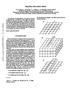
of Young diagrams, which we subsequently cast in the form of a coupled 4d/2d/0d system as in (1.1), by reorganizing the sums over the restricted diagrams into the integrals over gauge equivariant parameters and sums over magnetic fluxes of the partition functions of the two-dimensional theories τ L/R . This step heavily relies on factorization properties of the summand of instanton partition functions, which we derive in appendix C, when evaluated at special values of their gauge equivariant parameter. More importantly, we obtain concrete expressions for the instanton partition function, computing the equivariant volume of the instanton moduli space in the presence of intersecting codimension two singularities, and their corresponding ADHM matrix model. The main result of the paper, thus obtained, is the Sb4 -partition function of a four-dimensional N = 2 SU (N ) gauge theory with N fundamental and N antifundamental hypermultiplets,7 i.e., SQCD, in the presence of intersecting M2-brane surface defects, labeled by nR and nL -fold symmetric representations respectively. It takes the form (1.1) and can be found explicitly in (4.13). To be more precise, the coupled system we obtain involves chiral multiplets as zero-dimensional degrees of freedom, i.e., it coincides with the one described in conjecture 4 of [21] with four-dimensional N = 2 SQCD. The left subfigure in figure 1 depicts the 4d/2d/0d coupled system under consideration. We (T ,R2L ∪R2R ⊂R4 )

derive the instanton partition function Zinst

in the presence of intersecting planar surface

defects, which takes the form (T ,R2L ∪R2R ⊂R4 )

Zinst

=

X

2

2

~ R4 ~ R4 ~ ) z R4 (Y ~ ) z R L (Y ~ ) z RR (Y ~), q |Y | zvect (Y ) zafund (Y fund defect defect

(1.2)

~ Y

where we omitted all gauge and flavor equivariant parameters. It is expressed as the usual sum R2 ~ of Young diagrams. The summand contains the new fctors z L/R , which can be over N -tuples Y defect

found explicitly in (4.17), capturing the contributions to the instanton counting of the additional 4

R , zero-modes in the presence of intersecting surface defects, in addition to the standard factors zvect 4

4

R R zfund and zafund describing the contributions from the vector multiplet, and N + N hypermultiplets.

The coefficient of q k of the above result can be derived from the ADHM model for k-instantons depicted in right subfigure of figure 1. We have confirmed this ADHM model by analyzing the brane construction of said instantons, see section 5 for all the details. In section 6 we present conjectural generalizations of the instanton counting in the case of generic intersecting M2-brane defects. 7

While there is no distinction between a fundamental and antifundamental hypermultiplet, it is a useful terminology to keep track of the respective quiver gauge theory nodes. We choose to call the right/upper node of each link the fundamental one. 8 The partition function is insensitive to the presence of superpotential couplings.

4

N

N N

n

L

NS

n

N

R

ADHM

N

N

nL

k

nR

quiver 0d chiral 2d chiral 4d hyper

0d Fermi 0d chiral

Figure 1: On the left, the coupled 4d/2d/0d quiver gauge theory realizing the insertion, in fourdimensional N = 2 SQCD, of intersecting M2-brane surface defects labeled by symmetric representations of rank nR and nL respectively is depicted. The zero-dimensional multiplets are denoted using twodimensional N = (0, 2) quiver notation reduced to zero dimensions. Various superpotential couplings are turned on, in direct analogy to the ones given in detail in [21]. On the right, the ADHM model for k-instantons of the left theory is shown. The model preserves the dimensional reduction to zero dimensions of two-dimensional N = (0, 2) supersymmetry. We used the corresponding quiver conventions. A J-type superpotential equal to the sum of the U (k) adjoint bilinears formed out of the two pairs of chiral multiplets is turned on for the adjoint Fermi multiplet. The flavor charges carried by the various multiplets are also compatible with a quadratic J- or E-type superpotential for the Fermi multiplets charged under U (nL/R ).8

The paper is organized as follows. We start in section 2 by briefly recalling the Higgsing prescription to compute squashed sphere partition functions in the presence of (intersecting) M2brane defects labeled by symmetric representations. We also present its brane realization. In section 3 we implement the prescription for the case where T is a four- or five-dimensional theory of N 2 free hypermultiplets placed on a squashed sphere. The vacuum expectation value in T of intersecting M2-brane defects on the sphere has been computed in [21] from the point of view of the 4d/2d/0d or 5d/3d/1d coupled system and takes the form (1.1) (without the instanton contributions). For the case of symmetric representations, we reproduce this expression directly, and provide a derivation of a few details that were not addressed in [21]. We notice that the superpotential constraints of the coupled system on the parameters appearing in the partition function are reproduced effortlessly in the Higgsing computation thanks to the fact that they have a common origin in the theory Te ,

which in this case is SQCD. These relatively simple examples allow us to show in some detail the interplay of the various ingredients of the Higgsed partition function of theory Te , and how to cast it in the form (1.1). In section 4 we turn our attention to inserting defects in four-dimensional N = 2 SQCD. We apply the Higgsing prescription to an SU (N ) × SU (N ) gauge theory with bifundamental

hypermultiplets and for each gauge group an additional N fundamental hypermultiplets, and cast the resulting partition function in the form (1.1). As a result we obtain a sharp prediction for the instanton partition function in the presence of intersecting surface defects. This expression provides concrete support for the ADHM matrix model that we obtain in section 5 from a brane construction. We present our conclusions and some future directions in section 6. Five appendices contain various technical details and computations. 5

2

Higgsing and codimension two defects In this section we start by briefly recalling the Higgsing prescription to compute the partition

function of a theory T in the presence of (intersecting) defects placed on the squashed four/fivesphere [6, 7]. We also consider the brane realization of this prescription, which provides a natural bridge to the description of intersecting surface defects in terms of a 4d/2d/0d (or 5d/3d/1d) coupled system as in [21].

2.1

The Higgsing prescription

We will be interested in four/five-dimensional quantum field theories with eight supercharges.9 Let us for concreteness start by considering four-dimensional N = 2 supersymmetric theories. Consider a theory T whose flavor symmetry contains an SU (N ) factor, and consider the theory

of N 2 free hypermultiplets, which has flavor symmetry U Sp(2N 2 ) ⊃ SU (N ) × SU (N ) × U (1). By gauging the diagonal subgroup of the SU (N ) flavor symmetry factor of the former theory with one of the SU (N ) factors of the latter theory, we obtain a new theory Te . As compared to T , the theory Te has an extra U (1) factor in its flavor symmetry group. We denote the corresponding mass ˇ. parameter as M The theory Te can be placed on the squashed four-sphere Sb4 ,10 and its partition function can be

computed using localization techniques [27, 28]. Let us denote the supercharge used to localize the theory as Q. Its square is given by

Q2 = b−1 MR + bML − (b + b−1 )R + i

X

MJ FJ + gauge transformation ,

(2.1)

J

where MR/L are generators of the U (1)R/L isometries of Sb4 (see footnote 10), R is the SU (2)R

Cartan generator and FJ are the Cartan generators of the flavor symmetry algebra. The coefficients p ˜ where ` and `˜ are two radii of the squashed sphere (see MJ are mass parameters rescaled by ``,

footnote 10, to make them dimensionless. Localization techniques simplify the computation of the Sb4 partition function to the calculation of one-loop determinants of quadratic fluctuations around the localization locus given by arbitrary constant values for ΣT , the imaginary part of the vector e

9 The localization computations we will employ throughout this paper rely on a Lagrangian description, but the Higgsing prescription is applicable outside the realm of Lagrangian theories. We will restrict attention to (Lagrangian) four-dimensional N = 2 supersymmetric quantum field theories of class S and their five-dimensional uplift. 10 We consider Sb4 defined through the embedding equation in five-dimensional Euclidean space R5 = R × C2 with coordinates x, z1 , z2 |z1 |2 |z2 |2 x2 + 2 + =1, 2 r ` `˜2 in terms of parameters r, `, `˜ with dimension of length. The squashing parameter b is defined as b2 = ` . The isometries `˜

of Sb4 are given by U (1)R × U (1)L , which act by rotating the z1 and z2 plane respectively. The fixed locus of U (1)R is 2 2 a squashed two-spheres: SR = Sb4 z =0 and, similarly, the fixed locus of U (1)L is SL2 = Sb4 z =0 . The two-spheres SR 1 2 2 and SL intersect at their north pole and south pole, i.e., the points with coordinates z1 = z2 = 0 and x0 = ±r.

6

multiplet scalar of the total gauge group.11 The final result for the Sb4 partition function of the theory Te is then Z

(Te ,Sb4 )

where Zcl

(Te ,Sb4 )

(M ) =

Z

(Te ,Sb4 )

dΣT Zcl e

(Te ,S 4 )

(Te ,R4 )

(ΣT ) Z1-loopb (ΣT , M ) |Zinst e

e

(q, Σ, M  )|2 ,

(2.2)

(Te ,S 4 )

denotes the classical action evaluated on the localization locus, Z1-loopb is the one(Te ,R4 )

loop determinant and |Zinst

(q, Σ, M  )|2 are two copies of the Nekrasov instanton partition

function [29, 30], capturing the contribution to the localized path integral of instantons residing at the north and south pole of Sb4 . In [6,7], it was argued, by considering the physics at the infrared fixed point of the renormalization group flow triggered by a position dependent Higgs branch vacuum expectation value for the baryon constructed out of the hypermultiplet scalars, which carries charges ML = −nL , MR = −nR , R = e 4 N/2 and Fˇ = N , that the partition function Z (T ,Sb ) (M ) necessarily has a pole when −1 R L ˇ = b + b + b−1 n + b n . iM 2 N N

(2.3)

Moreover, the residue of the pole precisely captures the partition function of the theory T in the

presence of M2-brane surface defects labeled by nR -fold and nL -fold symmetric representations respectively up to the left-over contribution of the hypermultiplet that captures the fluctuations 2 , the fixed around the Higgs branch vacuum. These defects wrap two intersecting two-spheres SR/L

loci of U (1)R/L . 4

The pole at (2.3) of Z (T ,Sb ) (M ) finds its origin in the matrix integral (2.2) because of poles of e

the integrand pinching the integration contour. To see this, let us separate out the SU (N ) gauge group that gauges the free hypermultiplet to T , and split ΣT accordingly: ΣT = (ΣT , Σ), where ΣT e

e

is the vector multiplet scalar of the full gauge group of theory T , and Σ the SU (N ) vector multiplet scalar. We can then rewrite (2.2) as Z

(Te ,Sb4 )

(M ) =

Z

dΣ

T

Z

(Te ,Sb4 )

(T ,S 4 )

(Te ,R4 )

dΣ Zcl

(ΣT , Σ) Z1-loopb (ΣT , Σ, M ) |Zinst

N Y

N Y N Y

×

A,B=1 A6=B

Υb (i(ΣA − ΣB ))

A=1 I=1

(q, ΣT , Σ, M  )|2

 −1 Q ˇ)+ . (2.4) Υb i(ΣA − MI − M 2

The first factor in the second line is the one-loop determinant of the SU (N ) vector multiplet, while the second factor is the contribution of the N 2 extra hypermultiplets, organized into N SU (N ) fundamental hypermultipets.12 Here MI , I = 1, . . . , N denote the mass parameters associated to 11

More precisely, this is the “Coulomb branch localization” locus. Alternatively, one can perform a “Higgs branch localization” computation, see [15, 16]. 12 See appendix A for the definition and some useful properties of the various special functions that are used throughout the paper.

7

the SU (N ) flavor symmetry (with many others) located at

P

I

MI = 0). The integrand of the Σ-integral has poles (among

ˇ − nR b−1 − nL b − iΣA = iMσ(A) + iM A A

b + b−1 2

R/L

with

nA

≥0,

A = 1, . . . , N ,

(2.5)

where σ denotes a permutation of N variables. These poles arise from the one-loop determinant of ˇ takes the value of (2.3), they pinch the extra hypermultiplets. When the U (1) mass parameter M the integration contour if nR =

N X

nR A ,

nL =

A=1

N X

nLA ,

(2.6)

A=1

since we only have N − 1 independent SU (N ) integration variables. Note that the residue of the 4

pole of Z (T ,Sb ) at (2.3) is equal to the sum over all partitions of nR , nL in (2.6) of the residue of the e

4

Σ-integrand of Z (T ,Sb ) at the pole position (2.5) when treating the ΣA as N independent variables.13 A similar analysis can be performed for five-dimensional N = 1 theories. The theory Te can e

be put on the squashed five-sphere Sω~5 ,14 and its partition function can again be computed using localization techniques [31–36]. The localizing supercharge Q squares to 2

Q =

3 X

α=1

ωα M(α) − (ω1 + ω2 + ω3 )R + i

X

MJ FJ + gauge transformation ,

(2.8)

J

where M(α) are the generators of the U (1)(1) × U (1)(2) × U (1)(3) isometry of the squashed five-sphere

Sω~5 (see footnote 14). The localization locus consists of arbitrary constant values for the vector multiplet scalar ΣT , hence the partition function reads e

Z

5 (Te ,Sω ~)

(M ) =

Z

5 (Te ,Sω ~)

dΣT Zcl e

(Te ,S 5 )

(Te ,R4 ×S 1 )

(ΣT ) Z1-loopω~ (ΣT , M ) |Zinst e

e

(q, ΣT , M ω )|3 . e

(2.9)

5

One can argue that Z (T ,Sω~ ) (M ) has a pole at e

3

X n(α) ˇ = ω1 + ω2 + ω3 + iM ωα , 2 N

(2.10)

i=1

13

Upon gauging the additional U (1) flavor symmetry and turning on a Fayet-Iliopoulos parameter, which coincides with the gauged setup of [6,7], the residues of precisely these poles were given meaning in the “Higgs branch localization” computation of [16] in terms of Seiberg-Witten monopoles. 14 5 3 The squashed five-sphere Sω ~ =(ω1 ,ω2 ,ω3 ) is given by the locus in C satisfying ω12 |z1 |2 + ω22 |z2 |2 + ω32 |z3 |2 = 1 . (1)

(2)

(2.7)

(3)

Its isometries are U (1) × U (1) × U (1) , which act by rotations on the three complex planes respectively. The (α) 3 5 fixed locus of U (1)(α) is the squashed three-sphere S(α) = Sω × U (1)(β6=α) is the ~ zα =0 , while the fixed locus of U (1) 1 5 3 circle S(α∩β) = Sω ~ z =z =0 . The notation indicates that it appears as the intersection of the three-spheres S(α) and α

β

3 S(β) . A convenient visualization of the five-sphere and its fixed loci under one or two of the U (1) isometries is as a T 3 -fibration over a solid triangle, where on the edges one of the cycles shrinks and at the corners two cycles shrink simultanously.

8

whose residue computes the Sω~5 partition function of T in the presence of codimension two defects 3 obtained as labeled by n(α) -fold symmetric representations and wrapping the three-spheres S(α)

the fixed loci of the U (1)(α) isometries (see footnote 14), respectively. These three-spheres intersect each other in pairs along a circle. Again, this pole arises from pinching the integration contour by poles of the one-loop determinant of the N 2 hypermultiplets located at ˇ − iΣA = iMσ(A) + iM if n(α) =

PN

(α) A=1 nA .

3 X

α=1

(α)

n A ωα −

ω1 + ω2 + ω3 2

(α)

nA ≥ 0 ,

with

A = 1, . . . , N , (2.11)

5

The residue of Z (T ,Sω~ ) (M ) at the pole given in (2.10) equals the sum over e

partitions of the integers n(α) of the residue of the integrand at the pole position (2.11) with the ΣA treated as independent variables.15

2.2

Brane realization

To sharpen one’s intuition of the Higgsing prescription outlined in the previous subsection, one may look at its brane realization [7]. Consider a four-dimensional N = 2 gauge theory T described by the linear quiver and corresponding type IIA brane configuration16

N

N

···

N

←→

N

···

N D4

NS5

NS5

NS5

NS5

Gauging in a theory of N 2 hypermultiplets amounts to adding an additional NS5-brane on the right end of the brane array. The Higgsing prescription of the previous subsection is then trivially implemented by pulling away this additional NS5-brane (in the 10-direction of footnote 16), while suspending nR D2R and nL D2L -branes between the displaced NS5-brane and the right stack of D4-branes, see figure 2. Various observations should be made. First of all, the brane picture in figure 2 was also considered in [21] to describe intersecting M2-brane surface defects labeled by nR and nL -fold symmetric representations respectively. Its field theory realization is described by a coupled 4d/2d/0d system, described by the quiver in figure 3 (see [21]). Note that the two-dimensional 15 In [13], these residues were interpreted as the contribution to the partition function of K-theoretic Seiberg-Witten monopoles. 16 The branes in this figure as well as those in figure 2 and the following discussion span the following dimensions:

NS5 D4 D2L D2R D0

1 — — —

2 — — —

3 — —

4 — —

—

—

5 —

6 —

7

8

9

10

— — — —

9

...

N

N

D4

D4

N

D4

N

D4

...

N

NS5

NS5

N

D4

NS5

N

D4

D4

N

N

D4

N

D4

nL D2L

nR D2R

nR D2R

NS5

NS5

NS5

. . . D4

nL D2L

NS5

NS5

NS5

Figure 2: Gauging the diagonal subgroup of the SU (N ) flavor symmetry carried by the right-hand stack of D4-branes and an SU (N ) subgroup of the flavor symmetry of an additional N 2 free hypermultiplets amounts to adding an additional NS5-brane on the right end of the brane array. This leads to the figure on the left. Higgsing the system as in subsection 2.1 corresponds to pulling away this NS5-brane from the main stack, while stretching nR D2R and nL D2L -branes in between it and the D4-branes, producing the middle figure. The final figure represents the system in the Coulomb phase.

2dL nL N

N

···

0d

N

N

4d

nR 2dR Figure 3: Coupled 4d/2d/0d quiver gauge theory realizing intersecting M2-brane surface defects labeled by symmetric representations, of rank nR and nL respectively, in a four-dimensional N = 2 linear quiver gauge theory. The two-dimensional degrees of freedom, depicted in N = (2, 2) quiver notation, are coupled to the four-dimensional ones through cubic and quartic superpotential couplings. The explicit superpotentials can be found in [21]. The zero-dimensional degrees of freedom, denoted using two-dimensional N = (0, 2) quiver notations dimensionally reduced to zero dimensions, with solid lines representing chiral multiplets, participate in E- and J-type superpotentials.

theories, residing on the D2R and D2L -branes, are in their Higgs phase, with equal Fayet-Iliopoulos parameter ξFI proportional to the distance (in the 7-direction) between the displaced NS5-brane and the next right-most NS5-brane. Before Higgsing, this distance was proportional to the inverse square of the gauge coupling of the extra SU (N ) gauge node: ξFI =

4π . 2 gYM

(2.12)

In particular, the Higgsing prescription will produce gauge theory results in the regime where ξFI is positive, and where the defect is inserted at the right-most end of the quiver. In this paper we will restrict attention to this regime. Note however that sliding the displaced NS5-brane along the brane array in figure 2 implements hopping dualities [19, 37] (see also [38, 39]), which in the quiver gauge theory description of figure 3 translate to coupling the defect world volume theory to a different pair of neighboring nodes of the four-dimensional quiver, while not changing the resulting partition

10

function. In [21], a first-principles localization computation was performed to calculate the partition function of the coupled 4d/2d/0d system when placed on a squashed four-sphere, with the defects 2 , the fixed loci of U (1)R/L , in the case of non-interacting wrapping two intersecting two-spheres SR/L

four-dimensional theories. Our aim in the next section will be to reproduce these results from the Higgsing point of view. When the four-dimensional theory contains gauge fields, the localization computation needs as input the Nekrasov instanton partition function in the presence of intersecting planar surface defects, which modify non-trivially the ADHM data. The Higgsing prescription does not require such input, and in section 4 we will apply it to N = 2 SQCD. This computation will allow us to extract the modified ADHM integral.

The brane realization of figure 2 already provides compelling hints about how the ADHM data should be modified. In this setup, instantons are described by D0-branes stretching between the NS5-branes. Their worldvolume theory is enriched by massless modes (in the Coulomb phase, i.e., when ξFI = 0), if any, arising from open strings stretching between the D0-branes and the D2R and D2L -branes. These give rise to the dimensional reduction of a two-dimensional N = (2, 2) chiral multiplet to zero dimensions, or equivalently, the dimensional reduction of a two-dimensional N = (0, 2) chiral multiplet and Fermi multiplet. We will provide more details about the instanton counting in the presence of defects in section 5. Our Higgsing computation of section 4 will provide an independent verification of these arguments.

Intersecting defects in theory of N 2 free hypermultiplets

3

In this section we work out in some detail the Higgsing computation for the case where T is a

theory of free hypermultiplets. We will find perfect agreement with the description of intersecting M2brane defects labeled by symmetric representations in terms of a 4d/2d/0d (or 5d/3d/1d) system [21]. Our computation also provides a derivation of the Jeffrey-Kirwan-like residue prescription used to evaluate the partition function of the coupled 4d/2d/0d (or 5d/3d/1d) system, and of the flavor charges of the degrees of freedom living on the intersection. In the next section we will consider the case of interacting theories T .

3.1

Intersecting codimension two defects on Sω~5

As a first application of the Higgsing prescription of the previous subsection, we consider the partition function of a theory of N 2 free hypermultiplets on Sω~5 in the presence of intersecting 3 fixed by the U (1)(α) isometry (see codimension two defects wrapping two of the three-spheres S(α) 3 and S 3 . Our aim will be to cast the result in the manifest footnote 14, and also figure 4), say S(1) (2)

form of the partition function of a 5d/3d/1d coupled system, as in [21]. We consider this case 3 ∩ S3 = S1 first since the fact that the intersection S(1) (2) (1∩2) has a single connected component is a

11

1 S(1∩2)

b(1)

p

b(1) =

p

b(2) =

b(2)

p

b(3) = 3 S(1)

3 S(2)

Sω~5

b−1 (1) 1 S(1∩3)

b−1 (3)

ω1 /ω3 ω1 /ω2

1 S1∩2 : 1/ω3

b−1 (2)

3 S(3)

b(3)

radii

ω2 /ω3

1 S1∩3 : 1/ω2

1 S(2∩3)

1 S2∩3 : 1/ω1

Figure 4: A convenient representation of Sω~5 in terms of a T 3 -fibration over a triangle. Each edge represents a three-sphere invariant point-wise under one of the U (1) isometries, and each vertex represents an S 1 , where two S 3 ’s intersect, invariant point-wise under two U (1) isometries. Each S 1 has two tubular neighborhoods of the form S 1 × R2 in the two intersecting S 3 ’s, with omega-deformation parameters given in terms of b±1 (α) , as shown in the figure.

simplifying feature that will be absent in the example of Sb4 in the next subsection. Sω~5 partition function of Te

3.1.1

Our starting point, the theory Te , is described by the quiver

N

N

N

.

That is, it is an SU (N ) gauge theory with N fundamental and N anti-fundamental hypermultiplets, i.e., N = 2 SQCD.17 The S 5 -partition function of Te is computed by the matrix integral (2.9) ω ~

[31–36, 40, 41] Z

5 (Te ,Sω ~)

˜) = (M, M

Z

5 (Te ,Sω ~)

dΣ Zcl

5

4 ×S 1 )

(T ,S ) ˜ ) |Z (Te ,R (Σ) Z1-loopω~ (Σ, M, M inst e

˜  )|3 . (q, Σ, M  , M

(3.1)

The explicit expression for the classical action is given by 5 (Te ,Sω ~)

Zcl

 (Σ) = exp −

8π 3 Tr Σ2 2 ω1 ω2 ω3 gYM



,

(3.2)

(Te ,S 5 )

while the one-loop determinant Z1-loopω~ is the product of the one-loop determinants of the SU (N ) vector multiplet, the N fundamental hypermultiplets and the N antifundamental hypermultiplets: 5

5

5

5

(T ,S ) ˜ ) = Z Sω~ (Σ) Z Sω~ (Σ, M ) Z Sω~ (Σ, M ˜) Z1-loopω~ (Σ, M, M vect fund afund QN ~) A,B=1 S3 (i(ΣA − ΣB ) | ω A6=B = QN QN , Q QN ˜ ω |/2 | ω ~) N ω |/2 | ω ~) A=1 I=1 S3 (i(ΣA − MI ) + |~ A=1 J=1 S3 (i(−ΣA + MJ ) + |~ e

17

Recall our terminology of footnote 7.

12

(3.3) (3.4)

written in terms of the triple sine function. Here we used the notation |~ ω | = ω1 + ω2 + ω3 . Note that we did not explicitly separate the masses for the SU (N ) × U (1) flavor symmetry, but instead

considered U (N ) masses. Finally, there are three copies of the K-theoretic instanton partition function, capturing contributions of instantons residing at the circles kept fixed by two out of three U (1) isometries. Concretely, one has 1 (Te ,R4 ×S(2∩3) )

˜ ω 2π ω3 ω2  Σ Mω M , , , , , ω1 ω1 ω1 ω1 ω1 ω1 1 1 ˜ ω 2π ω3 ω1  (Te ,R4 ×S(1∩2) ˜ ω 2π ω1 ω2  (Te ,R4 ×S(1∩3) ) ) Σ Mω M Σ Mω M × Zinst , , , , Zinst , , , , , q2 , , q3 , , ω2 ω2 ω2 ω2 ω2 ω2 ω3 ω3 ω3 ω3 ω3 ω3 (3.5) (Te ,R4 ×S 1 )

|Zinst

˜ ω )|3 ≡ Z (q, Σ, M ω , M inst

 2 where qα = exp − g8π 2

YM

diagrams [29, 30]

~ = (Y1 , Y2 , . . . , YN ) , Y

2π ωα



q1 ,

. Each factor can be written as a sum over an N -tuple of Young

with YA = (YA1 ≥ YA2 ≥ . . . ≥ YAWYA ≥ YA(WY

A

+1)

= . . . = 0)

(3.6)

of a product over the contributions of vector and matter multiplets: 

 β β β ˜ω Σ, M ω , M , β, 1 , 2 2π 2π 2π      X ~ 4 1 β β ω R4 ×S 1 ~ β β ˜ω R4 ×S 1 ~ β |Y | R ×S ~ = q zvect Y , Σ zfund Y , Σ, M zafund Y , Σ, M . (3.7) 2π 2π 2π 2π 2π

(Te ,R4 ×S 1 )

Zinst

q,

~ Y

4

1

Here we have omitted the explicit dependence on 1 , 2 in all factors z R ×S . The instanton counting   2β ~ | denotes the total number of boxes in the N -tuple , and |Y parameter q is given by q = exp − 8π g2 YM

of Young diagrams. The expression for zfund reads R4 ×S 1 zfund

  Y   N Y N Y ∞ Y Ar Y β β ω β ω ~ Y , Σ, M = (iΣA − iMI ) + r1 + s2 , 2i sinh πi 2π 2π 2π

(3.8)

A=1 I=1 r=1 s=1

4

1

4

1

R ×S R ×S while those of zvect and zafund are given in (C.2)-(C.3) in appendix C.18 Note that the masses

that enter in (3.7) are slightly shifted (see [42]): i M ω ≡ M − (ω1 + ω2 + ω3 ) , 2

˜ω ≡ M ˜ − i (ω1 + ω2 + ω3 ) . M 2

18

(3.9)

In appendix C we have simultaneously performed manipulations of four-dimensional and five-dimensional instanton partition functions, which is possible after introducing the generalized factorial with respect to a function f (x), defined in appendix A.1, with f (x) in four and five dimensions given in (C.1).

13

3.1.2

Implementing the Higgsing prescription

As outlined in the previous subsection, to introduce intersecting codimension two defects 3 and S 3 and labeled by the n(1) -fold and n(2) -fold symmetric wrapping the three-spheres S(1) (2)

representation respectively, we should consider the residue at the pole position (2.11) with n(3) = 0 (3)

(and hence nA = 0 for all A = 1, . . . , N )19 (1)

(2)

iΣA = iMσ(A) − nA ω1 − nA ω2 −

ω1 + ω2 + ω3 2

for

A = 1, . . . , N ,

(3.10)

while treating ΣA as N independent variables, and sum over all partitions ~n(1) of n(1) and ~n(2) of n(2) . As before, σ(A) is a permutation of A = 1, ..., N which we take to be, without loss of generality, σ(A) = A. At this point let us introduce the notation that “→” means evaluating the residue at the pole (3.10) and removing some spurious factors. As we aim to cast the result in the form of a matrix integral describing the coupled 5d/3d/1d system, we try to factorize all contributions accordingly 3 or S 3 . As we will see, the in pieces depending only on information of either three-sphere S(1) (2)

non-factorizable pieces nicely cancel against each other, except for a factor that will ultimately describe the one-dimensional degrees of freedom residing on the intersection. It is straightforward to work out the residue at the pole position (3.10). The classical action (3.2) and the one-loop determinant (3.3) become, using recursion relations for the triple sine functions (see (A.8)),20 5 (Te ,Sω ~)

Zcl

(Te ,S 5 )

(T ,S 5 )

Z1-loopω~ → Z1-loopω~



S3

S3

(1) (1) Zcl|~ Z1-loop|~ n(1) n(1)

Let us unpack this expression a bit. First,



(T ,S 5 ) Z1-loopω~

S3

S3

(2) (2) Zcl|~ Z1-loop|~ n(2) n(2)



(1)

(2)

T ;~ n ,~ n Zcl,extra e

 Te ;~ n(1) ,~ n(2) Z1-loop,extra .

(3.11)

is the one-loop determinant of N 2 free hypermul-

tiplets, which constitute the infrared theory T . It reads (T ,S 5 ) Z1-loopω~

N Y N Y 1 1 = = . ˜ ˜J | ω S (−iMA + iMJ + |~ ω| | ω ~ ) A=1 J=1 S3 (iMA − iM ~) A=1 J=1 3 N Y N Y

(3.12)

Note that the masses of the N 2 free hypermultiplets, represented by a two-flavor-node quiver, are ˇ˜ while 1 PN iM = |~ω| + n(1) ω + n(2) ω . ˜ J + i |~ω| . Recall that 1 PN iM ˜ J = iM, MAJ = MA − M 1 2 A J=1 A=1 2 N N 2 N N Second, we find the classical action and one-loop determinant of squashed three-sphere partition

functions of a three-dimensional N = 2 supersymmetric U (n(α) ) gauge theory with N fundamental and N antifundamental chiral multiplets and one adjoint chiral multiplet, i.e., the quiver gauge theory 19

Recall that we have regrouped the mass for the U (1) flavor symmetry and those for the SU (N ) flavor symmetry into U (N ) masses. 20 Here we omitted on the right-hand side the left-over hypermultiplet contributions mentioned in the previous section as well as the classical action evaluated on the Higgs branch vacuum at infinity, i.e., on the position-independent Higgs branch vacuum.

14

N

N n(α)

We will henceforth call this theory ‘SQCDA.’21 These quantities are in their Higgs branch localized form,22 hence the additional subscript indicating the Higgs branch vacuum, i.e., the partition ~n(α) . (α)

Their explicit expressions can be found in appendix B.2. The Fayet-Iliopoulos parameter ξFI , (α)

(α)

(α)

the adjoint mass mX , and the fundamental and antifundamental masses mI , m ˜I

entering the

3 are identified with the five-dimensional parameters as three-dimensional partition function on S(α) q follows, with λ(α) ≡ ω(α) /(ω1 ω2 ω3 ),

8π 2 λ(α) (α) = , mX = iω(α) λ(α) , 2 gYM     i i (α) (α) ˜ J + (|~ ω | + ω(α) ) , m ˜ J = −iω(α) λ(α) + λ(α) M ω | + ω(α) ) . mI = λ(α) MI + (|~ 2 2

(α) ξFI

Note that the relation on the U (1) mass

1 N

PN

I=1 iMI

=

|~ ω| 2

+

n(1) N ω1

+

n(2) N ω2

(3.13) (3.14)

translates into a

relation on the U (1) mass of the fundamental chiral multiplets. Finally, both the classical action and the one-loop determinant produce extra factors which cannot be factorized in terms of information depending only on ~n(1) or ~n(2) , T˜ ;~ n(1) ,~ n(2) ~ n(1) ,~ n(2) ~ n(1) ,~ n(2) ˜) , Z1-1oop,extra = Zvf,extra (M ) Zafund,extra (M L

(1)

(2)

~ n ,~ n Zcl,extra = (q3 q¯3 )−

PN

A=1

(1) (2)

nA nA

,

(3.15)

R

~ n ,~ n where Zafund,extra captures the non-factorizable factors from the antifundamental one-loop deterL

R

~ n ,~ n minant, while Zvf,extra captures those from the vector multiplet and fundamental hypermultiplet

one-loop determinants, which can be found in (C.21)-(C.22). These factors will cancel against 21

Note that the rank of the gauge group is the rank of one of the symmetric representations labeling the defects supported on the codimension two surfaces, or in other words, it can be inferred from the precise coefficients of the pole of the Te partition function, see (2.10). 22 The squashed three-sphere partition function of a theory τ can be computed using two different localization schemes. The usual “Coulomb branch localization” computes it as a matrix integral of the schematic form [43–46] Z 3 (τ,S 3 ) (τ,Sb3 ) Z (τ,Sb ) = dσ Zcl b (σ) Z1-loop (σ) , while a “Higgs branch localization” computation brings it into the form [10, 11] 3

Z (τ,Sb ) =

X

(τ,S 3 )

(τ,S 3 )

(τ,R2 ×S 1 )

(τ,R2 ×S 1 )

b Zvortex|HV (b) Zvortex|HV (b−1 ) . Zcl|HVb Z1-loop|HV

HV

Here the sum runs over all Higgs vacua HV and the subscript |HV denotes that the quantity is evaluated in the Higgs R2 ×S 1 vacuum HV. Furthermore, one needs to include two copies of the K-theoretic vortex partition function Zvortex . The two expressions for Z are related by closing the integration contours in the former and summing over the residues of the enclosed poles. In the main text the theory τ will always be SQCDA and hence we omit the superscripted label. Note that for SQCDA, the sum over vacua is a sum over partitions of the rank of the gauge group. See appendix B for all the details.

15

factors produced by the instanton partition functions, which we consider next. When employing the Higgsing prescription to compute the partition function in the presence of defects, the most interesting part of the computation is the result of the analysis and massaging of the instanton partition functions (3.5) evaluated at the value (3.10) for their gauge equivariant parameter. We find that each term in the sum over Young diagrams can be brought into an almost factorized form. As mentioned before, certain non-factorizable factors cancel against the extra factors in (3.11), but a simple non-factorizable factor remains. When recasting the final expression in the form of a 5d/3d/1d coupled system, it is precisely this latter factor that captures the contribution 1 of the degrees of freedom living on the intersection S(1∩2) of the three-spheres on which the defects

live.

1 (Te ,R4 ×S(2∩3) )

Let us start by analyzing the instanton partition functions Zinst

1 (Te ,R4 ×S(1∩3) )

and Zinst

. It

1 (Te ,R4 ×S(2∩3) ) Zinst ,

is clear from (3.8) that upon plugging in the gauge equivariant parameter (3.10) in ~ has zero contribution if any of the Young diagrams YA has the N -tuple of Young diagrams Y 1 (Te ,R4 ×S(1∩3) )

(2)

more than nA rows. Similarly, Zinst

~ if any of its does not receive contributions from Y

(1)

members YA has more than nA rows. Hence the sum over Young diagrams simplifies to a sum over all possible sequences of n(α) non-decreasing integers. The summands of the instanton partition functions undergo many simplifications at the special value for the gauge equivariant parameter, and in fact one finds that they become precisely the K-theoretic vortex partition function for SQCDA upon using the parameter identifications (3.13) (see appendix C.2 for more details):23 1 (Te ,R4 ×S(2∩3) )

Zinst

R2 ×S 1

1 (Te ,R4 ×S(1∩3) )

(2∩3) → Zvortex|~ (b−1 ) , n(2) (2)

Zinst

R2 ×S 1

(1∩3) → Zvortex|~ (b−1 ) , n(1) (1)

(3.16)

with the three dimensional squashing parameters defined as b(1) ≡

p ω2 /ω3 ,

b(2) ≡

p ω1 /ω3 ,

1 (Te ,R4 ×S(1∩2) )

The third instanton partition function, Zinst

b(3) ≡

p ω1 /ω2 .

(3.17)

, behaves more intricately when substituting

the gauge covariant parameter of (3.5). From (3.8) one immediately finds that N -tuples of Young ~ have zero contribution if any of its constituting diagrams YA contain the “forbidden box” diagrams Y (1)

(2)

with coordinates (column,row) = (nA + 1, nA + 1). We split the remaining sum over N -tuples of Young diagrams into two, by defining the notion of large N -tuples, as those N -tuples satisfying the (1)

(2)

requirement that all of its members YA contain the box with coordinates (nA , nA ), and calling all other N -tuples small. Let us focus on the former sum first. 23 This fact has for example also been observed in [47–50], and can also be read off from the brane picture in figure 2. Before Higgsing, the instantons of the extra SU (N ) gauge node are realized by D0-branes spanning in between the NS5-branes. After Higgsing, the D0-branes can still be present if they end on the D2R and D2L -branes. If, say, nL = 0, they precisely turn into vortices of the two-dimensional theory living on the D2-branes.

16

mR ν 7

.. .

YL

YR

YR

4 3 2 1 0

=

Large Y

ν

mL µ YL 3 2 1 0 =µ

~ for n(1) = 4, n(2) = 8. The red box Figure 5: A constituent Y of a large N -tuple of Young diagrams Y (1) (2) denotes the “forbidden box” with coordinates (n + 1, n + 1). The green and blue areas denote Y L and Y R respectively. The definitions of mLµ and mR ν , see (3.19), are also indicated.

~ , we define Y ~ L and Y ~ R as the Young diagrams Given a large N -tuple Y (2)

L YAr = YAr − nA

R YAr = YA(n(1) +r)

(1)

for

1 ≤ r ≤ nA ,

for

1≤r.

A

(1)

L YAr =0

and

for nA < r

(3.18)

Furthermore, we define the non-decreasing sequences of integers mLAµ ≡ Y L

(1)

A(nA −µ)

,

(1)

˜R mR Aν ≡ Y

µ = 0, ..., nA − 1,

(2)

A(nA −ν)

,

(2)

ν = 0, ..., nA − 1 ,

(3.19)

where Y˜AR denotes the transposed diagram of YAR . Figure 5 clarifies these definitions. With these definitions in place, one can show (see appendix C.3) the following factorization of the summand of ~ the instanton partition function for large tuples of Young diagrams Y ~large | |Y

q3

1 (Te ,R4 ×S(1∩2) )

Zinst

2

 1 1 L R R2 ×S(1∩2) R2 ×S(1∩2) L R ~large → q |m |+|m | Z Y (m |b ) Z (1) (1) 3 vortex|~ n2 (m |b(2) ) vortex|~ n  e (1) (2) e (1) (2) −1 large|~ n(1) ,~ n(2) T ;~ n ,~ n T ;~ n ,~ n × Zintersection (mL , mR ) Zcl,extra Z1-loop,extra . (3.20)

1

R ×S Here we used Zvortex|~ n (m|b) to denote the summand of the U (n) SQCDA K-theoretic vortex partition

function, i.e., 2

1

R ×S Zvortex|~ n (b) =

X

|m|

2

1

R ×S zb Zvortex|~ n (m|b) ,

(3.21)

mAµ ≥0 mAµ ≤mA(µ+1)

where |m| =

P P A

µ mAµ .

large|~ n(1) ,~ n(2)

(See appendix B.2 for concrete expressions.) The factor Zintersection

17

is

given by large|~ n(1) ,~ n(2)

Zintersection ≡

N Y

(mL , mR )

(1)

(2)

nA −1 nB −1 

Y

A,B=1 µ=0

i−1 h β + µ) −  2i sinh πi i (MA − MB ) + 2 (mLAµ + ν) − 1 (mR 1 Bν 2π ν=0  h β i−1 × 2i sinh πi i (MA − MB ) + 2 (mLAµ + ν) − 1 (mR . (3.22) Bν + µ) + 2 2π Y

As announced, the extra factors in the second line of (3.20) cancel against those in (3.11). ~ R as in the second line of (3.18), but Y ~ L is not a proper For small diagrams, we can still define Y N -tuple of Young diagrams due to the presence of negative entries. Nevertheless, we can define sets of non-decreasing integers as (2)

mLAµ ≡ YA(n(1) −µ) − nA ,

(1)

0 ≤ µ ≤ nA − 1 ,

for

A

˜R mR Aν ≡ Y

(2)

A(nA −ν)

,

for

(2)

0 ≤ ν ≤ nA − 1 . (3.23)

It is clear that mLAµ can take negative values. Then one can show (see appendix C.4) that ~large | |Y

q3

1 (Te ,R4 ×S(1∩2) )

Zinst

 1 1 L R R2 ×S(1∩2) R2 ×S(1∩2) L R ~small → q |m |+|m | Z Y (m |b ) Z (1) (1) 3 vortex|~ n2 (m |b(2) ) (semi-)vortex|~ n  e (1) (2) e (1) (2) −1 ~ n(1) ,~ n(2) T ;~ n ,~ n T ;~ n ,~ n × Zintersection (mL , mR ) Zcl,extra Z1-loop,extra . (3.24)

The intersection factor for generic (small) N -tuples of Young diagrams is a generalization of R2 ×S 1

(1∩2) (3.22) that can be found explicitly in (C.25). The factor Z(semi-)vortex|~ (mL |b(1) ) is a somewhat n(1)

R2 ×S 1

(1∩2) complicated expression generalizing Zvortex|~ , which we present in (C.26). n(1)

Putting everything together, and noting that summing over all N -tuples of Young diagrams L/R

avoiding the forbidden box is equivalent to summing over all possible values of mAµ , we find the following result for the Higgsed partition function 5

(T ,S 5 )

Z (T ,Sω~ ) → Z1-loopω~ e

X0

~ large Y

+

large|~ n(1) ,~ n(2)

Z~n(1) (mL |b(1) ) Zintersection

X0

~ small Y

(mL , mR ) Z~n(2) (mR |b(2) )

~ n(1) ,~ n(2)

Zˆ~n(1) (mL |b(1) ) Zintersection (mL , mR ) Z~n(2) (mR |b(2) )

!

(3.25)

where S3

S3

|mL |

(1) (1) Z~n(1) (mL |b(1) ) = Zcl|~ Z1-loop|~ q n(1) n(1) 3

R2 ×S 1

R2 ×S 1

(1∩2) (1∩3) Zvortex|~ (mL |b(1) ) Zvortex|~ (b−1 ) , n(1) n(1) (1)

(3.26) R2 ×S 1

(1∩2) and similarly for Z~n(2) (mR |b(2) ). The expression for Zˆn1 (mL |b(1) ) is obtained by replacing Zvortex|n 1

18

R2 ×S 1

(1∩2) with Z(semi-)vortex|n . The prime on the sums over Young diagrams in (3.25) indicates that only 1

N -tuples of Young diagrams avoiding the “forbidden box” are included. To obtain the final result of the Higgsed partition function, we need to sum the right-hand side of (3.25) over all partitions ~n(1) of n(1) and ~n(2) of n(2) . 3.1.3

Matrix model description and 5d/3d/1d coupled system

Our next goal is to write down a matrix model integral that reproduces the Sω~5 -partition function of the theory T of N 2 free hypermultiplets in the presence of intersecting codimension two defects, i.e., a matrix integral that upon closing the integration contours appropriately reproduces the expression on the right-hand side of (3.25), summed over all partitions of n(1) and n(2) , as its sum over residues of encircled poles. A candidate matrix model is obtained relatively easily by analyzing the contribution of the large tuples of Young diagrams in (3.25). It reads (T ,S 5 )

Z

3 ∪S 3 ⊂S 5 ) (T ,S(1) ω ~ (2)

where Z

3 S(1)

(σ (1) )

=

Z1-loopω~

n(1) !n(2) !

Z

(1) n Y

JK a=1

dσa(1)

(2) n Y

(2)

dσb

Z

3 S(1)

(σ (1) ) Zintersection (σ (1) , σ (2) ) Z

3 S(2)

(σ (2) ) ,

b=1

(3.27)

denotes the classical action times the one-loop determinant of the

3 S(1)

partition

function of SQCDA, that is, of a three-dimensional N = 2 gauge theory with gauge group U (n(1) ), and N fundamental, N antifundamental and one adjoint chiral multiplet, and similarly for Z

3 S(2)

(σ (2) ).24

1 The contribution from the intersection S(1∩2) reads

Zintersection (σ

(1)

,σ

(2)

)=

(1) (2) n Y nY Y 

a=1 b=1 ± (2)

with ∆ab = −ib(2) σb (1)

 
 −1 1 2 2 2i sinh πi ∆ab ± b(1) + b(2) , 2

(3.28)

(1)

+ ib(1) σa . Note that from (3.13) we deduce that the Fayet-Iliopoulos

(2)

parameters ξFI and ξFI are both positive. The mass and other parameters on both three-spheres satisfy relations which follow from the identifications in (3.13)-(3.14). Concretely, we find (1)

   i (1) (2) b(1) mI + b(1) = b(2) mI + 2    i (1) (2) b(1) m ˜ J − b(1) = b(2) m ˜J − 2

(2)

b(1) ξFI = b(2) ξFI ,

(α)

(α)

i b 2 (2) i b 2 (2)

 

, ,

(1)

mX = i (2)

mX = i

b2(2) b(1) b2(1) b(2)

, (3.29) ,

(α)

where mI , m ˜ J and mX are the fundamental, antifundamental and adjoint masses on the respective spheres. Moreover, the differences of the relations in (3.14), for fixed α, relate the three-dimensional 3 to the five-dimensional mass parameters of the N 2 free hypermultiplets, mass parameters on S(α) 24

See appendix B.2 for concrete expressions for the integrand of the three-sphere partition function.

19

3d(2) n(2) N

1d

N

5d

n(1) 3d(1) Figure 6: Coupled 5d/3d/1d quiver gauge theory realizing intersecting M2-brane surface defects labeled by nR - and nL -fold symmetric representations in the five-dimensional theory of N 2 free hypermultiplets. The three-dimensional degrees of freedom are depicted in N = 2 quiver gauge notation, while the onedimensional ones are denoted using one-dimensional N = 2 quiver notations, with solid lines representing chiral multiplets. Various superpotential couplings are turned on, as in figure 3 (see [21]). Applying the Higgsing prescription to SQCD precisely results in the partition function of this quiver gauge theory.

˜ J + i |~ω| : i.e., to MIJ = MI − M 2   |~ ω| (α) (α) m − m ˜ − iωα + i MIJ = λ−1 . I J (α) 2

(3.30)

The matrix integral (3.27) is evaluated using a Jeffrey-Kirwan-like residue prescription [51]. We have derived it explicitly by demanding that the integral (3.27) reproduces the result of the Higgsing computation (see below). The prescription is fully specified by the following charge assignments: the matter fields that contribute to ZS 3 (σ (1) ) and ZS 3 (σ (2) ) are assigned their (1)

(1)

standard charges under the maximal torus U (1)n

(2)

(2)

× U (1)n

of the total gauge group U (n(1) ) ×

U (n(2) ), while all factors contributing to Zintersection (σ (1) , σ (2) ) are assigned charges of the form (1)

(2)

(0, . . . , 0, +b(1) , 0 . . . , 0 ; 0, . . . , 0, −b(2) , 0 . . . , 0). Furthermore, we pick the JK-vector η = (ξFI ; ξFI ), where we treat the Fayet-Iliopoulos parameters as an n(1) -vector and n(2) -vector respectively. Recall from (3.13) that both are positive. Before verifying that the matrix model (3.27), with the pole prescription just described, indeed faithfully reproduces the expression (3.25) summed over all partitions ~n(1) , ~n(2) , we remark that it takes precisely the form of the partition function of the 5d/3d/1d coupled system of figure 6, which is the trivial dimensional uplift of figure 3 specialized to the case of N 2 free hypermultiplets described by a two-flavor-node quiver. This statement can be verified by dimensionally uplifting (T ,S 5 )

the localization computation of [21]. In some detail, Z1-loopω~ captures the contributions to the partition function of the five-dimensional degrees of freedom, i.e., of the theory T consisting of N 2 free hypermultiplets, while Z

3 S(α)

3 , described by encodes those of the degrees of freedom living on S(α)

U (n(α) ) SQCDA, for α = 1, 2, and the factor Zintersection precisely equals the one-loop determinant 3 ∩ S3 = S1 of the one-dimensional bifundamental chiral multiplets living on the intersection S(1) (2) (1∩2) .

Moreover, the mass relations (3.30), which we find straightforwardly from the Higgsing prescription, are the consequences of cubic superpotential couplings in the 5d/3d/1d coupled system, which were 20

analyzed in detail in [21]. The mass relations among the (anti)fundamental chiral multiplet masses in (3.29) are in fact a solution of (3.30) obtained by subtracting the equation for α = 1 and α = 2 and subsequently performing a separation of the indices I, J. The separation constants appearing in the resulting solutions can be shifted to arbitrary values by performing a change of variables in the three-dimensional integrals, up to constant prefactors stemming from the classical actions. The Higgsing prescription also fixes the classical actions and hence we find specific values for the separation constants. The adjoint masses in (3.29) are the consequence of a quartic superpotential. Also observe that our computation fixes the flavor charge of the one-dimensional chiral multiplets, which enter explicitly in Zintersection , and for which no first-principles argument was provided in [21]. The integrand of (3.27) has poles in each of the three factors; the Jeffrey-Kirwan-like residue prescription is such that, among others, it picks out classes of poles, which we refer to as poles of type-ˆ ν . They read, for partitions ~n(1) and ~n(2) of n(1) and n(2) respectively, over all of which we (2)

sum, and for sequences of integers {ˆ νA } where νˆA ∈ {−1, 0, . . . , nA − 1}, (1)

(1)

(1)

µ = 0, . . . , nA − 1

(2)

(2)

(2)

ν = 0, . . . , nB − 1 .

poles of type-ˆ ν : σAµ = mA + µmX − imLAµ b(1) − inLAµ b−1 (1) , R −1 σBν = mB + νmX − imR Bν b(2) − inBν b(2) ,

(1)

(2)

(3.31)

L R L R where mLµ , mR ν , nµ , nν are non-decreasing sequences of integers, such that nAµ , nBν > 0 and (where

νˆ enters)   mL

Aµ≥0

 mL

Aµ≥1

≥0 ≥

mLA0

if νˆA = −1 = −ˆ νA − 1

if νˆA ≥ 0

,

mR 06ν6ˆ νA = 0 ,

mR ν≥ˆ νA +1 ≥ 0 .

(3.32)

Note that if all νˆA = −1 these poles are simply obtained by assigning to σ (1) a pole position of ZS 3

(1)

and to σ (2) a pole position of ZS 3 , whose residues precisely reproduce the sum over large diagrams (2)

in (3.25). Precisely this fact motivated the candidate matrix model in (3.27). In appendix D.2, we describe a simple algorithm to construct Young diagrams avoiding the “forbidden box” associated with poles of type-ˆ ν . Furthermore, we show in appendix D.3 that the sum over the corresponding residues precisely reproduce the sum over Young diagrams in (3.25). Finally, we show in appendix D.4 that the residues of poles not of type-ˆ ν , but contained in the Jeffrey-Kirwan-like prescription, cancel among themselves by studying a simplified example. We thus conclude that the integral (3.27) indeed faithfully reproduces the sum over Young diagrams in (3.25).

3.2

Intersecting surface defects on Sb4

Let us next study the partition function of N 2 free hypermultiplets on Sb4 in the presence of 2 , the fixed loci of the U (1)L/R intersecting codimension two defects wrapping the two-spheres SL/R 2 consists of two points. The analysis isometries (see footnote 10). The intersection of SL2 with SR

21

largely parallels the one in the previous subsection, so we will be more brief. Sb4 partition function of Te

3.2.1

The theory Te is an N = 2 supersymmetric gauge theory with gauge group SU (N ) and N

fundamental and N antifundamental hypermultiplets. Its squashed four-sphere partition function is computed by the matrix integral (2.2) (or (2.4)), Z

(Te ,Sb4 )

˜) = (M, M

Z

(Te ,Sb4 )

dΣ Zcl

4

4

(T ,S ) ˜ ) |Z (Te ,R ) (q, Σ, M  , M ˜  )|2 . (Σ) Z1-loopb (Σ, M, M inst. e

(3.33)

The classical action is given by (Te ,S 4 ) Zcl b (Σ)

  8π 2 2 = exp − 2 Tr Σ gYM

(3.34)

and the one-loop factor reads (Te ,S 4 )

S4

S4

S4

˜ ) = Z b (Σ) Z b (Σ, M ) Z b (Σ, M ˜) , Z1-loopb (Σ, M, M vect fund afund

(3.35)

where S4

b Zfund (Σ, M ) =

N Y N Y

I=1 A=1 S4

b ˜) = (Σ, M Zafund

1 , Υb (iΣA − iMI + Q/2)

S4

b Zvect (Σ) =

N Y

A,B=1 A6=B

Υb (iΣA − iΣB ) ,

N Y N Y

1 . ˜ J + Q/2) Υ (−iΣ + i M A b J=1 A=1

(3.36)

We have denoted the masses associated with the U (N ) flavor symmetry of the N fundamental ˜ J . We also denote hypermultiplets as MI and those of the N antifundamental hypermultiplets as M Q = b + b−1 . The instanton partition functions can be written as a sum over N -tuples of Young diagrams as 4

(Te ,R ) ˜ ) = Zinst. (q, Σ, M  , M

X

~ R4 ~ R4 ~ , Σ, M  , 1 , 2 ) z R4 (Y ~ , Σ, M ˜  , 1 , 2 ) . q |Y | zvect (Y , Σ, 1 , 2 ) zfund (Y afund

~ Y

(3.37)

The various factors in the summand are defined in (C.2) and (C.3) in appendix C. The Ω-deformation parameters are identified as 1 = b and 2 = b−1 , the superscript



denotes the usual shift of

hypermultiplet masses [42] i M  ≡ M − (1 + 2 ) , 2

˜ ≡ M ˜ − i (1 + 2 ) , M 2

and the modulus squared simply entails sending q = exp(2πiτ ) → q¯, with τ = 22

(3.38) ϑ 2π

+

4πi . 2 gYM

3.2.2

Implementing the Higgsing prescription

The Higgsing prescription instructs us to consider the poles of the fundamental one-loop factor given by

b + b−1 2

−1 iΣA = iMσ(A) − nLA b − nR − Ab

for

A = 1, . . . , N ,

(3.39)

with σ a permutation of N elements, which we choose to be the identity. At the end of the P L/R computation, we should sum over all partitions ~nL/R of nL , i.e., nL/R = A nA .

The fact that the two two-spheres intersect at two disjoint points, namely their north poles and

south poles, adds another layer of complication compared to the analysis in the previous subsection. Even so, when evaluating the residue at (3.39), the analysis of the classical action and one-loop determinants is straightforward. Both can be brought into a factorized form in terms of pieces depending only on information on either two-sphere, using the shift formula (A.11) for the latter, up to extra factors which will cancel against certain non-factorizable factors coming from the instanton partition functions. Explicitly, (Te ,Sb4 )

Zcl

(Te ,S 4 )

(T ,S 4 )

Z1-loopb → Z1-loopb



S2

S2

L L Zcl|~ Z1-loop|~ nL nL



S2

S2

R R Zcl|~ Z1-loop|~ nR nR



L

R

L

R

T ;~ n ,~ n T ;~ n ,~ n Zcl,extra Z1-loop,extra e

e

2

, (3.40)

(T ,S 4 )

where Z1-loopb is the one-loop determinant of N 2 hypermultiplets, which constitute the infrared S2

˜ J + i Q . Furthermore, Z L/RL/R denote factors in the theory T , and have masses MIJ = MI − M 2 . . . |~ n Higgs branch localized two-dimensional N = (2, 2) SQCDA two-sphere partition function (see

footnote 22 for the equivalent three-sphere discussion, and appendix B.1 for explicit expressions). The two-dimensional FI-parameter ξFI , fundamental masses mI , antifundamental masses m ˜ J and adjoint masses mX are related to the five-dimensional parameters as i ˜J + i , + ib2 , m ˜ LJ = bM mLX = ib2 (3.41) 2 2 i i −1 −1 ˜ −2 = ϑ + (nL/R − 1)π , mR + ib−2 , m ˜R , mR . (3.42) I = b MI + J = b MJ + X = ib 2 2

L R ξFI = ξFI =

ϑL/R

4π , 2 gYM

mLI = bMI +

Finally the extra factors are ~ nL ,~ nR ~ nL ,~ nR ~ nL ,~ nR ˜ ), Z1-loop,extra = Zvf,extra (M ) Zafund,extra (M L

R

L

Zcl,extra = (q q¯)−

PN

A=1

R nL A nA

,

(3.43)

R

~ n ,~ n ~ n ,~ n where Zvf,extra and Zafund,extra are as before the non-factorizable pieces produced by applying the

shift formulae to the (anti)fundamental one-loop determinant and can can be found in (C.21)-(C.22). The massaging of each of the two instanton partition functions, which now both describe instantons located at intersection points, is completely similar to the one we performed above. ~ can be restricted to a sum over tuples whose First, the sum over N -tuples of Young diagrams Y constituents YA all avoid the “forbidden” box at (nLA + 1, nR A + 1). Second, the left-over sum can be

23

decomposed into sums over large and small diagrams, and moreover their summands can almost be factorized in terms of the summands of vortex partition functions, after canceling some overall factors with the extra factors from the classical action and one-loop determinants in (3.40). The remaining non-factorizable factor is an intersection factor,

large|~ n(1) ,~ n(2)

Zintersection

N Y

(mL , mR ) =

(1)

(2)

nA −1 nB −1 

Y

Y

A,B=1 µ=0

ν=0



i(MA − MB ) + 2 (mLAµ + ν) − 1 (mR Bν + µ) − 1

× i(MA − MB ) + 2 (mLAµ + ν) − 1 (mR Bν + µ) + 2

−1

−1

. (3.44)

for large diagrams, and (C.25) for generic diagrams. The full expression for the residue at the pole location (3.39) thus involves the product of the two massaged instanton partition functions, together with the leftover classical action and one-loop determinant factors,  2  2  2 2 (T ,S 4 ) e 4 SL SL SR SR Z (T ,Sb ) → Z1-loopb Zcl|~ Z Z Z nL 1-loop|~ nL cl|~ nR 1-loop|~ nR X0 L R large|~ nL ,~ nR R2 L L R R2 R × q |m |+|m | Zvortex|~ L (m ) Zintersection (m , m ) Zvortex|~ n nR (m ) ~ large Y

+

X0

q

|mL |+|mR |

R2

Zsemi-vortex|~nL (mL )

~ nL ,~ nR Zintersection (mL , mR )

~ small Y

(3.45)

2 Zvortex|~nR (mR ) . R2

The final result for the Higgsed partition function is obtained by summing the right-hand side of this expression over all partitions ~nL/R of nL/R . 3.2.3

Matrix model description and 4d/2d/0d coupled system

As in the previous subsection, the contribution of large tuples in both instanton partition functions suggests the following matrix integral

Z

2 ∪S 2 ⊂S 4 ) (T ,SL R b

=

1 (T ,S 4 ) Z1-loopb L R n !n !

X Z

X

B R ∈ZnR B L ∈ZnL

R

L

n n Y dσaR Y dσcL S 2 R R 2 Z R (σ , B ) Z SL (σ L , B L ) JK a=1 2π c=1 2π Y ± × Zintersection (σ L , B L , σ R , B R ) , (3.46) ±

2

2 partition function for SQCDA with where Z SR (σ R , B R ) denotes the summand/integrand of the SR 2

gauge group U (nR ), and similarly for Z SL (σ L , B L ).25 The intersection factors read  −1 n Y n  Y b + b−1 b + b−1 ± ± = ∆ac + ∆ac − , 2 2 R

± Zintersection (σ L , B L , σ R , B R )

L

a=1 c=1

25

Concrete expressions can be found in appendix B.1.

24

(3.47)

2dR nR 0d

N

N

4d

nL 2dL Figure 7: Coupled 4d/2d/0d quiver gauge theory realizing intersecting M2-brane surface defects labeled by nR - and nL -fold symmetric representations in the four-dimensional theory of N 2 free hypermultiplets. Various superpotential couplings are turned on and are given in detail in [21]. The Higgsing prescription applied to SQCD precisely reproduces the partition function of this coupled system.

 −1 iσ R ± with ∆± = b a ac

BaR 2



 − b iσcL ±

BcL 2



and where b is the four-sphere squashing parameter.

The factor labeled by the plus sign arises from the intersection point at the north pole, and the other factor from the south pole. The mass and other parameters on both two-spheres satisfy relations, which can be derived from (3.41)-(3.42), 

  i = , b + = b mR I + 2    i =b m ˜R ϑL + nL π = ϑR + nR π , b−1 m ˜ LJ − J − 2 L ξFI

R ξFI

−1

mLI

 i , 2  i , 2

mLX = ib2 , (3.48) −2 mR , X = ib

˜ J + i Q are related to the two-dimensional mass while the hypermultiplet masses MIJ = MI − M 2 parameters as −1

ib



= MIJ

 i −1 ˜ LJ ) , + (b + b ) − b−1 (mLI − m 2



ib = MIJ

 i −1 + (b + b ) − b(mR ˜R I −m J ) . (3.49) 2

The residue prescription used to evaluate the integrals in (3.46) is completely similar to JeffreyKirwan-like prescription introduced in the previous subsection: the matter fields contributing to Z

2 SR/L

R

L

are assigned their natural charges under the Cartan subgroup U (1)n × U (1)n of the

total gauge group, while all factors of the intersection factors are assigned charges of the form (0, . . . , 0, b−1 , 0 . . . , 0 ; 0, . . . , 0, −b, 0 . . . , 0). The JK-vector is again given in terms of the FIR , ξ L ). We have derived this prescription by demanding that the matrix integral parameters, η = (ξFI FI

reproduces the result of the Higgsing computation. It was shown in [21] that the partition function of the 4d/2d/0d coupled system of figure 3 for the case of N 2 free hypermultiplets described by a two-flavor-node quiver, reproduced in figure 7 for Q ± convenience, precisely equals the matrix integral (3.46). In particular, ± Zintersection computes the one-loop determinant of the zero-dimensional bifundamental chiral multiplets at the two intersection 2 and S 2 . In the first-principles localization computation of [21], the points of the two-spheres SR L

25

relations (3.49) are consequences of cubic superpotential couplings. Up to separation constants, their solutions can be found to be the mass relations in (3.48). As explained in the previous subsection, the Higgsing computation fixes the separation constants to specific values. Note that our computations fixes the flavor symmetry charges of the zero-dimensional fields and provides a derivation of the residue prescription. The proof that the matrix integral reproduces the result of the Higgsing computation follows the same logic as the one in the previous subsection, but is substantially more involved due to the fact that two copies of the intersection factor are present. We present some of the details in appendix E.

4

Intersecting surface defects in interacting theories In the previous section, we have computed the expectation value of intersecting surface defects

in four-/five-dimensional theories T of free hypermultiplets placed on the four-/five-sphere. In this

section, we consider intersecting surface defects inserted in interacting theories. More precisely, we focus on T being an N = 2 supersymmetric theory with gauge group SU (N ) and N fundamental and N anti-fundamental hypermultiplets, i.e., N = 2 SQCD.

The partition function of SQCD on the four-sphere has appeared in our earlier computations, see

(3.33). In particular, it involves the contribution of instantons located at the north pole and south pole of the four-sphere. When decorating the computation with intersecting surface defects, which precisely have these points as their intersection locus, we should expect the instanton counting to be modified non-trivially. By performing the Higgsing procedure on a theory Te described by the N = 2 quiver

N

N

N

N

,

we will be able to derive a precise description of the modified ADHM integral by casting both the Higgsed partition function as well as its instanton contributions in a matrix integral form. The Sb4 -partition function of Te Z

(Te ,Sb4 )

˜,M ˆ) = (M, M

Z

N Y

is given by (Te ,Sb4 )

dΣA dΣ0B Zcl

4

(T ,S ) ˜,M ˆ) (Σ, Σ0 ) Z1-loopb (Σ, Σ0 , M, M

A,B=1

e

e 4 2 (T ,R ) ˜ , M ˆ  ) , (4.1) × Zinst. (q, q 0 , Σ, Σ0 , M  , M

˜ J denote the masses associated to the U (N ) flavor symmetry of the N fundamental where MI and M ˆ is the mass associated to the U (1) flavor and antifundamental hypermultiplets respectively, while M

26

symmetry of the bifundamental hypermultiplet. The classical action reads (Te ,S 4 ) Zcl b (Σ, Σ0 )

  8π 2 8π 2 2 02 , = exp − 2 Tr Σ − 02 Tr Σ gYM gYM

(4.2)

while the one-loop determinant is given by (Te ,S 4 )

S4

S4

S4

S4

S4

˜,M ˆ ) = Z b (Σ) Z b (Σ0 ) Z b (Σ, M ) Z b (Σ0 , M ˜ ) Z b (Σ, Σ0 , M ˆ ) , (4.3) Z1-loopb (Σ, Σ0 , M, M vect vect fund afund bifund where all factors were defined in (3.36) but Sb4 ˆ) Zbifund (Σ, Σ0 , M

=

N Y N Y

1

Υ (iΣ0B A=1 B=1 b

ˆ + Q/2) − iΣA + iM

.

(4.4)

The instanton partition function is given by a double sum over N -tuples of Young diagrams 4

(Te ,R ) ˜ , M ˆ ) = Zinst. (q, q 0 , Σ, Σ0 , M  , M

X

~

q |Y | q 0

~ 0| |Y

R4 R4 ~ 0 R4 ~ ~ , Σ, M  ) (Y , Σ0 ) zfund (Y (Y , Σ) zvect zvect

~ ,Y ~0 Y 4

4

R 0 ˆ ~ 0 , Σ0 , M ˜ ) zR ~ ~0 × zafund (Y bifund (Y , Y , Σ, Σ , M ) . (4.5)

The contributions of the various multiplets can be found in appendix C. The superscripts



again

denote the usual shift [42] ˜ = M ˜ − i (1 + 2 ) , M 2

i M  = M − (1 + 2 ) , 2

ˆ = M ˆ − i (1 + 2 ) . M 2

(4.6)

Implementing the Higgsing prescription once again amounts to considering the poles of the fundamental one-loop factor given by −1 iΣA = iMσ(A) − nLA b − nR − Ab

b + b−1 2

for

A = 1, . . . , N ,

(4.7)

with σ a permutation of N elements, which we choose to be the identity. Here ~nL/R is a partition of nL/R , and we will sum over all. It is straightforward to compute the residues of the one-loop determinant at (4.7): (Te ,Sb4 )

Zcl

Here

(Te ,S 4 )

(T ,Sb4 )

Z1-loopb → Zcl

(T ,S 4 ) (T ,S 4 ) Zcl b Z1-loopb

(T ,S 4 )

Z1-loopb



S2

S2

L L Zcl|~ Z1-loop|~ nL nL



S2

S2

R R Zcl|~ Z1-loop|~ nR nR



L

R

L

R

T ;~ n ,~ n T ;~ n ,~ n Zcl,extra Z1-loop,extra e

e

2

,

(4.8)

are the classical action and one-loop determinant of the theory T , i.e., of

four-dimensional N = 2 supersymmetric SQCD. Their expression can be found in (3.34) and (3.35) ˜ J , but the fundamental respectively.26 The antifundamental masses of T are simply given by M 26

In the previous section the theory Te was SQCD.

27

masses take the values ˆ + iQ/2 MA0 = MA − M

(4.9) S2

in terms of the fundamental and bifundamental masses of the quiver theory Te . As before, Z. .L/R . |~ nL/R

denote factors in the Higgs branch localized SQCDA two-sphere partition function. The twoL/R

L/R

L/R

dimensional FI-parameters ξFI , fundamental masses mI adjoint masses

L/R mX

and

i 4π ˆ)+ i , , mLI = b(MI + iQ/2) + b2 , m ˜ LJ = b(Σ0J + M mLX = ib2 (4.10) 2 2 2 gYM i −2 i 4π −1 −1 0 −2 ˆ , m ˜R , mR , (4.11) = 2 , mR I = b (MI + iQ/2) + b J = b (ΣJ + M ) + X = ib 2 2 gYM

L ξFI = R ξFI

, antifundamental masses m ˜J are now related to the four-dimensional parameters of theory Te as

together with ϑL/R = θ + (nL/R − 1)π. Note that the two-dimensional masses depend on the fourdimensional gauge parameter. The explicit expressions for the extra one-loop factors, which now

receives contributions from the fundamental hypermultiplet, vector multiplet and bifundamental hyL

R

~ n ,~ n permultiplet one-loop determinant, can be found in (C.22)-(C.23). Again, Zcl,extra = (q q¯)−

P

A

R nL A nA .

When substituting the gauge equivariant parameter (4.7) in the instanton partition functions ~ avoiding the “forbidden box” and (4.5), the only non-vanishing contributions arise from N -tuples Y ~ 0 . As before, we can split the sum over the former into one over large and one arbitrary N -tuples Y over small tuples. As we have learned in the previous section, the analysis of the large tuples is sufficient to derive the matrix model integral describing the infrared system, i.e., the theory T with intersecting defects inserted. We thus focus only on such large tuples. We find ~

~ 0|

q |Ylarge | q 0|Y

1 (Te ,R4 ×S(1∩2) )

Zinst

~ 0, Y ~large ) (Y

2 2 ~˜ 0 , Σ0 , mR ) R4 ~ 0 R4 ~ 0 , Σ0 , M ˜  ) z R4 (Y ~ 0 , Σ0 , M 0 ) z RL (Y ~ 0 , Σ0 , mL ) z RR (Y zvect (Y , Σ0 ) zafund (Y fund defect defect  e (1) (2) e (1) (2) −1 large|~ nL ,~ nR T ;~ n ,~ n T ;~ n ,~ n R2 L L R R2 R × q |mL |+|mR | Zvortex|~ (m ) Z (m , m ) Z (m ) Zcl,extra Z1-loop,extra , intersection nL vortex|~ nR

~ 0|

→ q 0|Y

(4.12)

R2

L/R The intersection factor was already given in (3.44). The expression for the factors zdefect can be

found in (C.20). They clearly correspond to new ingredients in the instanton partition function of T , arising due to the presence of the defects on the local R2L/R . Momentarily, we will study the

modified ADHM data and its corresponding ADHM integral computing this modified instanton partition function. Recall that to obtain the final expression for the Higgsed partition function, we need to sum over all partitions of nL/R .

28

A matrix model integral describing the Sb4 partition function of SU (N ) SQCD in the presence 2 of intersecting surface defects supported on SL, R can be inferred from (4.8) and (4.12) to be Z

2 2 (T ,SL ∪SR ⊂Sb4 )

1 = L R n !n !

2 SR

2 SL

X Z

X

dΣ

B R ∈ZnR B L ∈ZnL

0

Z

L

R

n n Y dσaR Y dσbL (T ,Sb4 ) 0 (T ,S 4 ) ˜) Zcl (Σ ) Z1-loopb (Σ0 , M 0 , M 2π JK a=1 2π b=1

− × Z (σ R , B R ; Σ0 ) Z (σ L , B L ; Σ0 ) Zintersection (σ L , B L , σ R , B R ) (4.13) 2 X 0 2 2 ~ | R4 |Y ~ 0 , Σ0 ) z R4 (Y ~ 0 , Σ0 , M ˜  ) z R4 (Y ~ 0 , Σ0 , M 0 ) z RL (Y ~ 0 , Σ0 , σ L , B L ) z R R ( Y ~ 0 , Σ0 , σ R , B R ) . q 0 zvect (Y × afund fund defect defect Y~ 0 + Zintersection (σ L , B L , σ R , B R )

Here the factors in the first lines are the classical action and one-loop determinant of T , i.e., 2 four-dimensional SQCD, and the factors in the second line are the SL/R partition functions for

SQCDA as well as the intersection factors (3.47). The last line contains two copies of the instanton partition function, computed in the presence of the locally planar intersecting surface defects. The mass parameters on the two two-spheres are related as in (3.48), while the parameters of the four-dimensional theory T are related to the two-dimensional ones as −1

ib

=



MI0

−

Σ0J

 i −1 + (b + b ) −b−1 (mLI − m ˜ LJ ) , 2

ib =



MI0

−

Σ0J

 i −1 + (b + b ) −b(mR ˜R I −m J) . 2 (4.14)

Note that when performing the integral over the four-dimensional gauge parameter Σ0 , one should use m ˜ LJ = bΣ0J + m ˜ LU (1) , L/R

where m ˜ U (1) =

1 N

PN

L/R ˜K . K=1 m

−1 0 m ˜R ˜R J = b ΣJ + m U (1) ,

(4.15)

These follow directly from (4.14). In the two-dimensional one-loop

determinants we have made explicit this Σ0 -dependence. Note that by performing the change of L/R

variables σI

L/R

→ σI

L/R

+m ˜ U (1) in the two-dimensional integrals, one effectively changes the U (1)

L/R

L/R

L/R

L/R

masses as m ˜ U (1) → 0 and mU (1) → mU (1) − m ˜ U (1) in the matrix integral, up to an overall constant factor originating from the two-dimensional classical actions.27 Henceforth, we choose to work with this effective new integral. The contribution of the locally planar surface defect, supported on the local R2L , to the north pole copy of the instanton partition function is given by WY 0

0

n Y N Y B Y Br Y Y 1 L −2 (iσa + Ba /2 − im ˜ B ) + r1 + s2 + B )= , 2 −2 (iσa + Ba /2 − im ˜ B ) + (r − 1)1 + s2 L

R2L ~ 0 , Σ0 , iσ L zdefect (Y

(4.17)

a=1 B=1 r=1 s=1

27

Note that in terms of the effective variables, the relation (4.14) remains unaffected,        i i i R −1 L b−1 mL + = b m + + c , b m ˜ − = b m ˜R I J − I J 2 2 2

−1 i with c = b−1 m ˜L ˜R ). U (1) − bm U (1) + 2 (b − b

29

but (3.48) is modified as  i +c, (4.16) 2

2dR nR N

0d

N

N

4d

nL 2dL Figure 8: Coupled 4d/2d/0d quiver gauge theory realizing the insertion, in four-dimensional N = 2 SQCD, of intersecting M2-brane surface defects labeled by symmetric representations of rank nR and nL respectively . Various superpotential couplings are turned, in direct analogy to the ones given in detail in [21]. The Higgsing prescription applied to a linear quiver gauge theory with two gauge nodes reproduces the partition function of this coupled system. R2

R where WYB0 denotes the width of the Young diagram YB0 . Similarly, zdefect is obtained by swapping 1 L ↔ R, 1 ↔ 2 and YB ↔ Y˜B . The combination iσ + B is valid for the north pole contributions;

2

to get the south pole counterpart one replaces it with iσ − 12 B.

One can verify that if we perform the integrations over σ L/R and the sums over B L/R using the

same Jeffrey-Kirwan-like residue prescription as discussed in the previous section, the matrix model (4.13) reproduces the result obtained from the Higgsing prescription. The 4d/2d/0d coupled system

whose partition function is computed by (4.13) is depicted

in figure 8. The first line of (4.13) captures the classical action and one-loop determinant of the four-dimensional theory, while the second line captures the contributions of the two-dimensional degrees of freedom residing on the intersecting two-spheres as well as the one-loop determinants of the zero-dimensional bifundamental chiral multiplets at their intersection points. The most salient new feature of this coupled system is the fact that part of the two-dimensional flavor symmetry is gauged by the four-dimensional gauge symmetry. This fact is reflected in the relations in (4.14), relating the two-dimensional mass parameters m ˜ to the gauge parameter Σ0 , which are the consequence of the usual cubic superpotential couplings. As mentioned above, when computing the squashed four-sphere partition function of the coupled system, the instanton counting is modified non-trivially due to the presence of the intersecting surface defects. The argument of the modulus squared in the last line of (4.13) provides a concrete expression for the modified instanton partition function. In the next section, we turn to a more detailed analysis of the degrees of freedom which give rise to this instanton partition function.

30

N

D4

N

0 kD

N

D4

N N

nL D2L nL

D4

N k

nR

R

n D2R NS5

NS5

NS5 Figure 9: The left part of the figure depicts the brane configuration realizing k-instantons in N = 2 SQCD, in the presence of intersecting surface defects, of M2-type and labeled by symmetric representations, represented by the gray branes.28 The right part of the figure shows the quiver description of the worldvolume theory of the D0-branes. As the system preserves two-dimensional N = (0, 2) supersymmetry dimensionally reduced to zero dimensions, the quiver is drawn using N = (0, 2) notations, with full lines representing chiral multiplets and dashed lines Fermi multiplets. In the absence of the defects, the preserved supersymmetry is N = (0, 4). We thus learn that one needs to turn a J-type superpotentials JΛ for the adjoint Fermi multiplet Λ consisting of the sum of the adjoint bilinears of the scalars of the two pairs of chiral multiplets. The charges in table 1 are also compatible with quadratic E- or J-type superpotentials for the Fermi multiplets charged under U (nL/R ).

5

Instanton partition function and intersecting surface defects Let us start by considering the familiar brane realization of a k-instanton in SU (N ) N = 2

SQCD as an additional stack of k D0-branes as depicted in the the left part of figure 9, ignoring the gray branes for the time being.

The supersymmetry preserved by the worldvolume theory

of the D0-branes is the dimensional reduction to zero dimensions of two-dimensional N = (0, 4) supersymmetry. Its matter content can be straightforwardly read off by quantizing the open strings

stretching between the D0-brane and the various D4-branes, as well as between the D0-branes themelves, see [52, 53]. We summarize it in table 1, and have depicted the resulting quiver gauge theory in the right part of figure 9 (omitting the gray quiver nodes and links). The partition function of this zero-dimensional theory computes the (non-perturbative) k-instanton partition function, 4

which we denote as ZkR . In some more detail, the instanton partition function of a four-dimensional N = 2 supersymmetric

theory is computed by a localization computation on R41 ,2 , i.e., in the Ω-background parametrized by 1 , 2 [29, 30]. The localizing supercharge Q squares to Q2 = (1 + 2 )(Jr + R) + (1 − 2 )Jl + iΣ · G + iM · F ,

(5.1)

where Jl , Jr are the Cartan generators of the SU (2)l × SU (2)r ' SO(4) rotational symmetries 28

The brane directions are as in footnote 16.

31

strings

D0-D41

D0-D42

D0-D43

N = (0, 4)

FM

HM

FM

N = (0, 2)

FM

CM

CM

J

0

1 2

1 2

0

Jl

0

0

0

0

FM

D0-D0 VM VM

HM

FM

CM

CM

0

1

0

0

1 2 1 2

1 2 1 −2

D0-D2R

D0-D2L

(not preserved)

(not preserved)

CM

FM

CM

0

1 2

0

1 2

1 2

0

− 12

0

FM

Table 1: Massless excitations of strings stretching between the branes indicated in the first row organized in multiplets of the dimensional reduction of two-dimensional N = (0, 4) and N = (0, 2) supersymmetry to zero dimensions in the second and third row respectively. Here VM denotes vectormultiplet, HM hypermultiplet, FM Fermi multiplet and CM chiral multiplet. Note that the system including the D2-branes only preserves N = (0, 2), hence we leave the N = (0, 4) entries corresponding to D0-D2 strings open. The last two rows list the charges of the mutliplets under the flavor symmetry charges J and Jl .

of R4 ,29 while R is the SU (2)R generator. We define J = Jr + R. Furthermore, G denotes

the collection of Cartan generators of the gauge symmetry and F those of the flavor symmetry; φ and M are their respective equivariant parameters. The localization locus consists of pointinstantons located at the origin. The integration over the k-instanton moduli space is captured by the non-perturbative k-instanton partition function, which equals the partition function of the zero-dimensional ADHM model, read off as the worldvolume theory on the D0-branes, computed by localization with respect to the induced supercharge, that is, with respect to the supercharge in its N = (0, 2) supersymmetry (sub)algebra satisfying the same square as in (5.1) (up to gauge transformations). From the N = (0, 2) zero-dimensional point of view, the charges J = Jr + R and Jl appear as flavor charges, as do both G and F . Q2 additionally includes φ · G0d .

Dimensionally reducing the localization results of [54] and in particular [55], it is now straight4

forward to compute ZkR as 4 ZkR

=

Z

k Y

JK I=1

˜ ) ZD0-D4 (φ, Σ0 ) ZD0-D4 (φ, M ) , dφI ZD0-D0 (φ) ZD0-D41 (φ, M 2 3

(5.2)

29 The Ω-deformation breaks the rotational symmetry to SO(2)1 × SO(2)2 . In terms of their Cartan generators J1 , J2 one has Jl = 12 (J1 − J2 ) and Jr = 12 (J1 + J2 ).

32

where ZD0-D0 (φ) =

k Y (φIJ )0 (φIJ + 1 + 2 ) , (φIJ + 1 )(φIJ + 2 )

(5.3)

I,J=1

˜) = ZD0-D41 (φ, M ZD0-D42 (φ, Σ0 ) =

k Y N Y

I=1 A=1 k Y N Y

I=1 A=1

˜ A) , (φI − iM

(φI −

iΣ0A

+

ZD0-D43 (φ, M ) =

k Y N Y

I=1 A=1

1 2 (1

(φI − iMA ) ,

(5.4)

1 , + 2 ))(−φI + iΣ0A + 21 (1 + 2 ))

(5.5)

where φIJ = φI − φJ , and the prime on (φIJ )0 indicates to omit the factors with I = J. Here we denoted the equivariant parameters for the various SU (N ) symmetries as in the previous section.

The integral (5.2) is computed using the Jeffrey-Kirwan residue prescription. We choose to select the contributions of negatively charged fields, and thus collect the residues of the poles defined by solving the equations 1 φI = iΣ0A + (1 + 2 ), 2

φI = φJ + 1 ,

φI = φJ + 2 .

~ = {YA } such that The contributing poles are labeled by N -tuples of Young diagrams Y 1 φI = iΣ0A − (1 + 2 ) + r1 + s2 , 2

(r, s) ∈ YA .

(5.6) P

A |YA |

= k,

(5.7)

It is easy to convince oneself that summing over the residues precisely reproduces the q k term of the SQCD instanton partition function given in (3.37). Let us now re-introduce the intersecting surface defects in the setup.30 The brane configuration was already depicted in the left part of figure 9, now also considering the gray branes. Upon inserting the defects, the N = (0, 4) symmetry, dimensionally reduced to zero dimensions, carried

by the D0-branes is broken to the dimensional reduction of N = (0, 2). We have used precisely this subalgebra in the previous paragraphs already. The zero-dimensional model is enriched by the

modes arising from the quantization of the open strings stretching between the D0 and D2L and D2R -branes. They each contribute an additional N = (0, 2) Fermi and chiral multiplet,31 and the

final ADHM quiver theory is depicted in the right part of figure 9. The additional multiplets carry charges under J and Jl as in table 1. It is then straightforward to include their contributions to the 30 See also [7] for an analysis of the equivariant integral of a five-dimensional theory in the presence of threedimensional chiral multiplets. 31 The brane system consisting of a stack of D0-branes and one stack of D2-branes, each ending on an NS5-brane, preserves on the D0-brane the dimensional reduction to zero dimensions of N = (2, 2) supersymmetry. The open string modes thus organize themselves in an N = (2, 2) chiral multiplet.

33

ADHM matrix model. It is given by ZD0-D2 (φ, Σ0 , σ, B) " nL −1 K Y N A Y Y (φI − 2 (iσaL + ≡ L a=0 (φI − 2 (iσa + I=1 A=1 L/R

where we used σa

L/R

− i Ba2

BaL 2 ) BaL 2 )

R

nA −1 + 21 (1 + 2 ) Y (φI − 1 (iσaR +

− 21 (1 − 2 )

a=0

(φI − 1 (iσaR +

BaR 2 ) BaR 2 )

+ 21 (1 + 2 ) + 21 (1 − 2 )

#

. (5.8)

as the gauge equivariant parameter of the U (nL/R ) symmetry, as

this is the combination that enters in our computations on Sb4 at the north pole. (The south pole contribution would be obtained by changing the sign in front of B.)32 Noting that our JK-prescription does not select the poles of the above factor, it is straightforward to see that the matrix integral R2 ∪R2 ⊂R4 Zk L R

=

Z

k Y

JK I=1

˜ ) ZD0-D4 (φ, Σ0 ) ZD0-D4 (φ, M ) ZD0-D2 (φ, Σ0 , σ, B) dφI ZD0-D0 (φ) ZD0-D41 (φ, M 2 3 (5.9)

precisely reproduces the modified instanton partition function as it appeared in the last line of (4.13).

6

Discussion In this paper, we have extended the study of intersecting codimension two defects, initiated

in [21], to interacting four-dimensional theories. We have employed the Higgsing prescription of [6,7] to compute the vacuum expectation value of intersecting M2-brane defects, labeled by nL and nR -fold symmetric representations respectively, inserted in four-dimensional N = 2 SQCD, which

we abbreviate to T . Subsequently we cast the result in the form of a partition function of a coupled 4d/2d/0d system, see (4.13), which takes the schematic form33 Z

2 ∪S 2 ⊂S 4 ) (T ,SL R b

=

Z X

(T ,S 4 )

2) (τ L ,SL

Zpert b Zpert

2) (τ R ,SR

Zpert

(T ,R2L ∪R2R ⊂R4 ) 2 + − Zintersection Zintersection Zinst . (6.1)

The leftmost subfigure of figure 10 depicts the 4d/2d/0d coupled system under consideration and identifies τ L/R as two-dimensional N = (2, 2) U (nL/R ) SQCDA. Our computation provides

an explicit formula for the instanton partition function in the presence of the above-mentioned (T ,R2L ∪R2R ⊂R4 )

intersecting defects, Zinst

, appearing in (6.1), see equation (4.13). We also found the (T ,R2L ∪R2R ⊂R4 )

ADHM model whose partition function computes the k-instanton contribution to Zinst

,

see the rightmost subfigure in figure 10. This model can be read off from a D-brane construction, as 32

Note that we are using the effective description obtained by performing a change of variables in the two-dimensional integrals and omitting some irrelevant constant prefactor as explained below equation (4.13). 33 Before tackling this computation, we also considered the theory of N 2 free hypermultiplets. Also for this case, we cast the result in the form of a partition function of a coupled system.

34

N

N

N D4 n

L

NS

n

N D4

R

N

N D4 D4,D2

N

N

nL D2L

k D0

worldvolume

D0

nL

k

nR

worldvolume R

n D2R

0d chiral 2d chiral 4d hyper

N

NS5

NS5

0d Fermi 0d chiral

NS5

Figure 10: The type IIA brane-configuration in the middle describes the 4d/2d/0d coupled system on the left as the worldvolume theory of the D4/D2L /D2R -branes, see also figure 8. The worldvolume theory of the k D0-branes is shown on the right, see figure 9 for more details. Its partition function computes the k-instanton partition function of the 4d/2d/0d coupled system.

N D4 N D4

N D4

NS5

NS5

nL2

nL1

N

nR 2

nR 1

N D4

N D4

N D4

N

NS5

NS5

nL2 D2L

nL1 D2L

nR 2 D2R

nR 1 D2R NS5

NS5

Figure 11: One starts with the theory T of N 2 free hypermultiplets and successively gauges in two more theories of N 2 free hypermultiplets. The brane realization of the resulting theory Te is shown in the leftmost figure. One can then apply the Higgsing prescription twice, corresponding to pulling the R two rightmost NS5-branes away from the main stack, and stretching (nL2 − nL1 , nR 2 − n1 ) (D2L , D2R ) L R branes and (n1 , n1 ) (D2L , D2R ) branes respectively in between them and the flavor D4- branes. The two-dimensional part of the system is in its Higgs phase, and can be brought into its Coulomb phase by aligning the two displaced NS5-branes, as shown in the middle figure. The corresponding 4d/2d/0d coupled system can be read off easily, and is shown in the last figure. This system was also considered in [21].

also indicated in the figure. Starting from a theory T whose flavor symmetry contains an SU (N ) factor, one can gauge in successively multiple, say p, theories of N 2 free hypermultiplets. The resulting theory Te has p

additional U (1) factors in its flavor symmetry group compared to the original theory T . It is clear

that one can apply the Higgsing prescription consecutively to each of these starting from the one at outermost along the quiver. The associated type IIA brane-realization is a simple generalization of the one we have discussed in section 2.2. We depict the case p = 2 for T the theory of N 2

free hypermultiplets in figure 11. The corresponding 4d/2d/0d coupled system can be read off from the brane picture and is given in the rightmost subfigure in figure 11. We conjecture that the M-theory interpretation of this procedure corresponds to the insertion of multiple intersecting M2-branes ending on the main stack of M5-branes, describing theory T , all labeled by symmetric representations.

General intersecting M2-brane defects labeled by two generic irreducible representations (RL , RR ) 35

nL nL W L −2 W L −1 D2L

nLW L D2L

D2L

...

nR W R D2R

· · 34 · · · · · 10 N

NS5L

NS5L

NS5L

· · 3456 · 89 · N ···

nL W L −1

2 ,D me D4 olu v rld wo

nLW L 0d Fermi nR WR N N

nR W R −1

N

D4

nR nR W R −1 W R −2 D2R

D2R

12 · · · · · · · 10 D4

N D4

NS5

0 k D 123456 · · · ·

NS5

...

NS5R

NS5R NS5R

12 · ·56 · 89 · D0 dv olu me

wo rl

···

N N

nLW L

N k

nR WR

0d Fermi 0d chiral 0d Fermi 2d chiral 4d hyper

Figure 12: The type IIA brane realization of general intersecting M2-brane defects labeled by two irreducible representation (RL , RR ) inserted in SQCD, as well as its corresponding 4d/2d/0d coupled system and ADHM model are depicted.

of SU (N ) can also be described by 4d/2d/0d coupled systems [21]; when the four-dimensional theory is N = 2 SQCD, we have depicted an example in the bottom left of figure 12. The two-dimensional

degrees of freedom are described by quiver gauge theories which encode the representation R through

their gauge group ranks [19]. The coupled system involves zero-dimensional Fermi multiplets, transforming in the bifundamental representation of the innermost two-dimensional gauge groups, as degrees of freedom living at the intersection points. Such 4d/2d/0d coupled system can be engineered as the worldvolume theory of the D4/D2L /D2R -branes in the type IIA system shown in figure 12. When attempting to use this coupled system to compute the vacuum expectation value of general intersecting M2-brane defects, one needs as an input the instanton partition function in the presence of the defects. We propose that the structure of its k-instanton ADHM model can also in this case be read off from the D0-brane worldvolume theory in the type IIA system. The resulting quiver theory, which has two-dimensional N = (0, 2) supersymmetry reduced to zero dimensions, is also

included in figure 12. It is almost the same as the one in figure 10, up to the orientation of an arrow. This new ADHM model however leads to a dramatically different ADHM integration: extra poles coming from the factor ZD0-D2 will be selected by the JK-prescription, and the result of the ADHM integral is a double sum over N -tuples of Young diagrams and, separately, nL -tuples of Young diagrams, together having k boxes in total. It would be very interesting to study in more detail these new ADHM integrals. When RL/R are both symmetric representations, the descriptions of figures 12 and 10 are 36

both valid. In [21], the equality of the resulting squashed four-sphere partition functions was verified for four-dimensional theories without gauge fields, and for defects labeled by fundamental representations. It would be of interest to study the duality between the two descriptions in interacting theories. A construction for general intersecting M2-brane defects in terms of a renormalization group flow from a larger theory Te triggered by some position-dependent Higgs branch vacuum expectation

value is currently unknown. Presumably it requires Te to be a non-Lagrangian theory of class S. Reversing the logic, one might hope to recover information about the partition function of the UV non-Lagrangian theory Te by investigating the partition function of all intersecting M2-brane defects, for which we have nice quiver description, and to which the UV theory can flow. Note that Higgs branch localized expressions of partition functions are a simple example of this aspiration [16].

It was conjectured in [21] that the partition function of SU (N ) SQCD in the presence of general intersecting M2-brane defects can be identified with Liouville/Toda five-point functions. In particular, identifying x0 = qz, x = z, with |q|, |z| < 1, along with other parameter identifications, one expects

D E 2 2 4 ˜ ) = A(x, x0 ) Vˆα (0) Vˆ−bΩ −b−1 Ω (x0 ) Vˆβ (x) Vˆα (1) Vˆα∞ (∞) , Z (T ,SL ∪SR ⊂Sb ) (q, z, M 0 , M 0 1 RL RR

(6.2)

where A(x, x0 ) ≡ A|x0 |2γ0 |1 − x0 |2γ1 |x|2γ2 |1 − x|2γ3 |x − x0 |2γ4 , for some γi . Furthermore α0 , α∞ are

generic, while β, α1 are semi-degenerate momenta determined in terms of the masses of the gauge theory. Let us perform a few checks of this statement, leaving a more thorough analysis for the future. R

Consider the simple case with RL = 1 and RR = symmn 2. In the OPE limit 1 > |q| > |z| → 0,

the leading terms in z read, up to the factor A, X t

−1 t)−2∆(α

|z|2∆(α0 −b

Here t =

PN

R A=1 nA hA

0 )−2∆(−n

R b−1 h ) 1

D E −b−1 t ˆ ˆ ˆ ˆ Cˆαα00,−n V (0) V (x) V (1) V (∞) . −1 α1 α∞ β R b−1 h α0 −b t 1

(6.3)

and hA are the weights of the fundamental representation of SU (N ). The

set of natural numbers ~nR is any partition of nR , and the sum over t means summing over all such partitions. On the gauge theory side, in the z → 0 limit, one can close the contour of the 2

4

integration over σ R in the partition function Z (T ,SR ⊂Sb ) , as in (4.13) with nL = 0, and obtain

the Higgs branch localized expression as a sum over the two-dimensional Higgs vacua labeled by partitions ~nR . This sum is mapped to the sum over t in (6.3). The leading terms in z simply come from the zero-vortex sector. The four-dimensional matrix integral in each leading term, which now depends on the Higgs vacuum ~nR , is simply an Sb4 -partition function with shifted fundamental

37

Z

Sb4

N

N

N

N

!



AGT

Vα0 Vβ 0 Vβ Vα1 Vα∞

Degeneration

Higgsing

ˇ →M ˇ nL ,nR M

β 0 → −nL bh1 − nR b−1 h1 nR

Z

2 2 SL ∪SR ⊂Sb4

N



N

N

!

hVα0 V−nL bh1 −nR b−1 h1 Vβ Vα1 Vα∞ i

nL

Figure 13: A commuting diagram showing the relation between the Higgsing prescription and degenerating semi-degenerate momentum. R ˆ + i(b + b−1 )/2 + inR b−1 , thanks to masses MAn ≡ MA0 − M A 2

4

R4 ~ 0 , M 0 ε ) z RR ⊂R (Y ~ 0 , Σ0 , iσ R , B R ) → z R4 (Y ~ 0 , (M nR )ε ) , zfund (Y fund defect

(6.4)

where → indicates the evaluation at the Higgs vacuum ~nR . This Sb4 -partition function is mapped to

the four-point function in (6.3). In particular, the four-dimensional one-loop determinant together

with the two-dimensional one-loop determinant evaluated at the Higgs vacuum ~nR is precisely equal −1 to the structure constants Cˆ α0 −b R t−1 Cˆ α −1 Cˆα,α ,α∞ , up to some uninteresting constants. α0 ,−n b

h1

α0 −b

In fact, the statement (6.2) in the case of

t,β

RL/R

1

being both symmetric, can be viewed as a

degeneration of the well-established AGT conjecture without surface defects, by considering the ˇ nL ,nR = (bnL + b−1 nR )/N + commuting diagram in figure 13 [47–49]. We remind ourselves that iM h i P (b + b−1 )/2, and in the AGT correspondence β 0 = N (b + b−1 )/2 − N iM h1 . The Higgsing A A=1 L R ˇ → M ˇ n ,n , which is equivalent to degenerating the semiprescription sends the U (1) mass M degenerate momentum β 0 → −nL bh1 − nR b−1 h1 .

The correspondence (6.2) is a great tool to discover and understand new dualities of the 4d/2d/0d

coupled system. The Liouville/Toda correlation functions enjoy various symmetries, including, but not limited to, the invariance under conjugation and Weyl reflection of the momenta, and conformal and crossing symmetries. It would be interesting to translate these CFT symmetries to dualities on the gauge theory side, especially when the intersecting defects are coupled to four-dimensional interacting theories.

Acknowledgments The authors would like to thank Giulio Bonelli, Jaume Gomis, Bruno Le Floch, Fabrizio Nieri, Daniel Park, Massimiliano Ronzani, Alessandro Tanzini, Maxim Zabzine for helpful conversations

38

and useful suggestions. Y.P. is supported in part by Vetenskapsr˚ adet under grant #2014- 5517, by the STINT grant and by the grant “Geometry and Physics” from the Knut and Alice Wallenberg foundation. The work of W.P. is supported in part by the DOE grant doe-sc0010008.

A

Special functions In this appendix we briefly recall the definitions and some useful properties of the special

functions which play an essential role in this paper.

A.1

Factorials

In analyzing vortex and instanton partition functions, one often encounters products of the form Qm−1 k=0 f1 ,2 (z + k), for some function f1 ,2 . Due to its frequent occurrence and to streamline the discussion we introduce the factorial

(z)fm

≡

m−1 Y

f1 ,2 (z + k) .

As a trivial example, it includes the standard Pochhammer symbol (x)m ≡ f1 ,2 = id. We often abbreviate f1 ,2 as f when no confusion is expected.

A.2

(A.1)

k=0

Qm−1 k=0

(x + k), for

Double- and triple-sine functions

Double-sine function sb (z):

the double-sine function sb (z) is defined as the regularized version

of the product sb (z) ≡

Y (m + 1/2)b + (n + 1/2)b−1 − iz . (m + 1/2)b + (n + 1/2)b−1 + iz

(A.2)

m,n>0

It is a common practice to define Q ≡ b + b−1 . The function sb (z + iQ/2) has poles at z =

+im≥0 b + in≥0 b−1 and zeros at z = −im≥1 b − in≥1 b−1 . The double sine function satisfies the following recursion relation

  mn iQ   (−1) s z + b 2 iQ Qn sb z + + imb + inb−1 = Qm , 2 2i sinh πb(z + ikb) 2i sinh πb−1 (z + ikb−1 ) k=1 k=1

(A.3)

as well as the symmetry properties sb (z) sb (−z) = 1 ,

    iQ iQ 1 sb z + sb −z + = . 2 2 2 sinh(πbz) 2 sinh(πb−1 z)

39

(A.4)

An alternative definition of the double-sine function is given by S2 (z|ω1 , ω2 ) ≡

Y

m,n≥0

mω1 + nω2 + z . (m + 1)ω1 + (n + 1)ω2 − z

The definitions of sb (z) and S2 (z|ω1 , ω2 ) are related by b =   z Q , S2 (z|ω1 , ω2 ) = sb −i + i √ 2 ω1 ω2 Triple-sine function S3 (z|~ ω ):

S2



p

(A.5)

ω1 /ω2 and

   ω1 + ω2 z . − iz ω1 , ω2 = sb √ 2 ω1 ω2

(A.6)

the triple-sine function S3 (z|~ ω ) for any triplet ω ~ = (ω1 , ω2 , ω3 ) is

defined as the regularization of the product +∞ Y

S3 (z|~ ω) =

n1 ,n2 ,n3 =0

(z + ~n · ω ~ ) ((~n + 1) · ω ~ − z) .

(A.7)

It has no poles, and its zeros are located at z = (~n + 1) · ω ~ or z = −~n · ω ~ for nα ≥ 0. It satisfies a convenient recursion relation (where S1 (z|ω) ≡ 2 sinh(πz/ω)) S3

z+

3 X

α=1

= (−1)

n1 n2 n3

nα ωα |ω1 , ω2 , ω3

S3 (z|ω1 , ω2 , ω3 )

!

nY 1 −1 k1 =0

×

nY 2 −1 nY 3 −1 k2 =0 k3 =0

nY nY 2 −1 3 −1 1 1 1 S2 (z + k1 ω1 |ω2 , ω3 ) S2 (z + k2 ω2 |ω1 , ω3 ) S2 (z + k3 ω3 |ω1 , ω2 ) k2 =0

S1 (z + k2 ω2 + k3 ω3 |ω1 )

nY 2 −1 1 −1 nY k1 =0 k2 =0

S1 (z + k1 ω1 + k2 ω2 |ω3 )

k3 =0

nY 3 −1 1 −1 nY k1 =0 k3 =0

S1 (z + k1 ω1 + k3 ω3 |ω2 ) , (A.8)

and has the following symmetry property S3 (z|~ ω ) = S3 (ω1 + ω2 + ω3 − z|~ ω) .

A.3

(A.9)

Υb functions

The function Υb (z) is defined as Υb (z) =

Y

(mb + nb−1 + z)((m + 1)b + (n + 1)b−1 − z) .

m,n≥0

40

(A.10)

It has no poles, but zeros located at z = −mb − nb−1 and z = (m + 1)b + (n + 1)b−1 , for m, n ≥ 0, and satisfies the recursion relation for m, n ∈ Z

Qm Qn −1 2 −1 2 r=0 s=0 (z + rb + sb ) r=1 s=1 (z − rb − sb ) Υb (z − mb − nb ) = (−1) Υb (z) Q−m−1 Qn Qm Q−n−1 −1 2 −1 2 r=0 s=1 (z + rb − sb ) r=1 s=0 (z − rb + sb ) Q Q Q−m−1 Q−n−1 m n −1+2(z−rb)b 1−2(z−sb−1 )b−1 γ(b(z + rb)) s=0 γ(b−1 (z + sb−1 )) r=1 b s=1 b r=0 Q × Q Q Q n m −n−1 1−2(z+sb−1 )b−1 . −m−1 −1+2(z+rb)b −1 −1 b s=1 γ(b (z − sb )) r=1 γ(b(z − rb)) s=0 b r=0 −1

Q−m−1 Q−n−1

|mn|

(A.11)

Here we defined Q ≡ b + b−1 , and for each product, when the lower limit is strictly larger than the

upper limit, the product reduces to 1. Some other useful properties include Υb (Q − z) = Υb (z) and

Υb (Q/2) = 1.

The S 2 and Sb3 SQCDA partition function

B

In this appendix we briefly recall the two-dimensional N = (2, 2) supersymmetric and three-

dimensional N = 2 supersymmetric sphere partition function of a U (nc ) gauge theory with nf

fundamental, naf antifundamental, and one adjoint chiral multiplet, which we henceforth call SQCDA, and present its Higgs branch localized form. Here and in the next appendices, we will use the notation (i, µ) in substitution of the original P color index a ∈ {1, ..., nc }, where i = 1, ..., nf , µ = 0, ..., ki − 1, with i ki = nc . Each partition ~k = {ki } corresponds to a Higgs vacuum of the theory. Therefore, for arbitrary functions Φ of arbitrary sequences of nc variables xa , we have nc Y

a=1

B.1

Φ(xa ) →

nf kY i −1 Y i=1 µ=0

Φ(xiµ ) ≡

Y

Φ(xiµ ) ,

(i,µ)

nc X a=1

Φ(xa ) →

nf kX i −1 X i=1 µ=0

Φ(xiµ ) ≡

X

Φ(xiµ ) . (B.1)

(i,µ)

The S 2 SQCDA partition function

The two-sphere partition function of an N = (2, 2) supersymmetric gauge theory with gauge

group U (nc ) and with nf fundamental chiral multiplets with masses mj , naf antifundamental chiral multiplets with masses m ˜ t and an adjoint chiral multiplet with mass mX is computed by [8, 9] S2

ZSQCDA

" #  Z Y nc  2 1 X dσa −4πiξFI σa −iϑBa Y (B − B ) a b = e (σa − σb )2 + nc ! 2π 4 nc B∈Z

a=1 nf Y nc Y

×

×

a>b naf Y nc Ba Γ(−iσa − 2 + imj ) Y Γ(+iσa + B2a − im ˜ t) Ba Ba Γ(1 + iσa − 2 − imj ) t=1 a=1 Γ(1 − iσa + 2 + im ˜ t) j=1 a=1 n c b Y Γ(−iσa + iσb − Ba −B + imX ) 2 . Ba −Bb Γ(1 + iσa − iσb − 2 − imX ) a,b=1

41

(B.2)

Here we have set the r-charges to zero. They can be reinstated by analytically continuing the masses. In comparison to higher-dimensional sphere partition functions, the two-sphere partition function also involves a sum over magnetic fluxes B. We have also included the two-dimensional ϑ-angle in the classical action. The one-loop determinants for the chiral multiplets are expressed in terms of the standard Gamma-function. Finally, note that we have turned off background fluxes for the flavor symmetries, as they will play no role in this paper. Assuming that nf > naf or nf = naf with ξFI > 0, we can close the integration contours of (B.2) in the lower half-plane. The integrand of the σ-integrations in (B.2) is an infinite sum over B ∈ Znc . One can show that the sum of the residues of different permutations of the color label give the same result, canceling the nc ! in (B.2). For each summand with a given Ba , the relevant poles are then given by iσjµ = imj + µmX + Njµ +

|Bjµ | , 2

for all

0 ≤ Nj0 ≤ Nj1 ≤ ... ≤ Nj(kj −1) ∈ N ,

(B.3)

Pnf where µ = 0, ..., kj − 1, and ~k is a partition of nc : j=1 kj = nc , labeling the Higgs vacua. These poles can be rewritten into a more useful form, by introducing mjµ = Njµ + njµ = Njµ +

|Bjµ | 2

−

Bjµ 2 .

poles of type σm,n :

Bjµ 2

+

|Bjµ | 2 ,

We collectively denote these poles as σm,n , iσjµ +

Bjµ = imj + µimX + mjµ , 2

iσjµ −

Bjµ = imj + µimX + njµ . 2 (B.4)

Note that m, n are sequences of non-decreasing natural numbers, such that 0 ≤ mj0 ≤ mj1 ≤ ... ≤

mj(kj −1) , 0 ≤ nj0 ≤ nj1 ≤ ... ≤ nj(kj −1) , ∀j = 1, ..., nf . Alternatively, one can solve N and B in terms of m, n by definition.

The sum over residues can be brought into the form [19] 2

S ZSQCDA =

X

2

2

S S Zcl| ~k Z1-loop|~k

k

X m

2

R zˆ|m| Zvortex| ~k (m)

X n

|n| R2 zˆ¯ Zvortex| ~k (n) ,

(B.5)

0

where zˆ is defined as zˆ = e−2πξFI +iϑ , with ϑ0 = ϑ + π(nf − naf + nc + 1). Furthermore, we introduced P |m| ≡ jµ mjµ , and similarly for |n|. The classical and one-loop factors read, with mjl ≡ mj − ml and m ˜ jt ≡ mj − m ˜ t,



Zcl|~k = exp −4πiξFI

2

S Z1-loop| ~k =

nf  X j=1

Qnf Qnf Qkj −1

  mX kj mj + (kj − 1)kj  2

µ=0 γ(−imjl + nl imX − µimX ) l=1 , Qnf Qnaf Qkj −1 ˜ jt − µimX ) t=1 µ=0 γ(1 − im j=1

j=1

42

(B.6)

(B.7)

where γ(x) =

Γ(x) Γ(1−x) .

R2 Zvortex| ~k (m)

The summand Z R

nf kY naf Y j −1 Y

=

t=1 j=1 µ=0

×

nf Y

j,l=1

P m

B.2

of the vortex partition function is given by

(1 − i(mj − m ˜ t ) − µimX − mjµ )mjµ

" kj −1 k −1 l Y Y µ=0 ν=0

1 (1 − imjl − (µ − ν)imX + mlν − mjµ )mjµ −mjµ−1

Y (1 + imjl − (kl − µ)imX + mjµ − ml(kl −1) )ml(k −1)

kj −1

× and

2

(m) vortex|~k

l

(1 + imjl − (kl − µ)imX )mjµ

µ=0

(B.8) #

,

denotes a sum over all possible non-decreasing sequences of natural numbers mj .

The Sb3 SQCDA partition function

The squashed three-sphere is defined by its embedding in C2 as ω12 |z1 |2 + ω22 |z2 |2 = 1 , and the parameter b is given by b =

(B.9)

p ω2 /ω1 . The partition function of an N = 2 supersymmetric

gauge theory with gauge group U (nc ) and with nf fundamental chiral multiplets with masses mj , naf antifundamental chiral multiplets with masses m ˜ t and an adjoint chiral multiplet with mass mX is computed by [43–46]

Z

Sb3

1 = nc !

Z

nc Y

dσa

a=1

!

e−2πiξFI Tr σ

Y

a>b

2 sinh(πb(σa − σb )) 2 sinh(πb−1 (σa − σb ))

  iQ   nc s + σ − m ˜ Y a t t=1 a=1 b 2 iQ   − σa + σb + mX , (B.10) ×Q sb nf Qnc iQ 2 s − + σ − m a j a,b=1 a=1 b j=1 2 Qnaf Qnc

where Q = b + b−1 and the matter one-loop determinants are expressed in terms of the double-sine function sb . We have taken the Chern-Simons level to be zero. When nf > naf or nf = naf and the FI-parameter ξFI > 0,34 we again consider poles of type σm,n

in the lower half-plane, labeled by ascending sequences of natural numbers 0 ≤ mj0 ≤ mj1 ≤ ... ≤ mj(kj −1) , ∀j = 1, ..., nf , poles of type σm,n :

σiµ = mj + µmX − imjµ b − injµ b−1 , µ = 0, ..., kj − 1, mjµ , njµ ∈ N . (B.11)

Summing over the residues, one obtains the Higgs branch localized Sb3 -partition function [10, 11], 34 Note that if we had turned on a Chern-Simons level, the convergence criterion would have been slightly more subtle than in two dimensions, as was explained in [11].

43

with Higgs vacua specified by a partition ~k, Sb3 ZSQCDA

=

X k

S3 Z b~ cl|k

Z

Sb3

1-loop|~k

" X m

2 1 |m| zb Z R ×S ~ vortex|k

(m|b)

# " X n

2 1 |n| zb−1 Z R ×S ~ vortex|k

−1

n|b




#

,

(B.12)

where the classical and 1-loop factors, with mij ≡ mi − mj , are given by Z Z

Sb3 cl|~k

Sb3

1-loop|~k

i h Xnf mX Xnf (kj − 1)kj mj kj + ≡ exp 2πiξFI j=1 j=1 2   n naf Y f YY Y iQ iQ sb sb ( ≡ − mlj + (kj − µ)mX + mj − m ˜ t + µmX ) . 2 2 2 ×S 1

vortex|~k

2 1 Z R ×S ~ vortex|k

(m|b) ≡

(m|b) of the vortex partition function is given by

naf Y nf kY j −1 Y t=1 j=1 µ=0

×

(B.14)

t=1 (j,µ)

j=1 (l,µ)

The summand Z R

(B.13)

nf Y

j,l=1

(1 − ib−1 (mj − m ˜ t ) − iµb−1 mX − mjµ )fmjµ

" kj −1 k −1 l Y Y

+ mlν − mjµ )fmjµ −mj,µ−1 # kj −1 Y (1 + ib−1 mjl − i(kl − µ)b−1 mX + mjµ − ml,kl −1 )fml,k −1 l

µ=0 ν=0

×

1 (1 −

ib−1 m

− i(µ −

(1 + ib−1 mjl − i(kl − µ)b−1 mX )fmjµ

µ=0

Here we used the function (x)fm ≡

jl

Qm−1 k=0

(B.15)

ν)b−1 mX

.

f (x + k) with f (x) = 2i sinh πib2 x. See appendix

A. Expression (B.15) is summed over all possible sequences of non-decreasing natural numbers 0 ≤ mj0 ≤ mj1 ≤ ... ≤ mj(kj −1) , with weighting factor given in terms of zb±1 ≡ e−2πξFI b

B.3

±1

|m| ≡

Xnf Xkj −1 j=1

µ=0

mjµ .

(B.16)

Forest-tree representation

The poles (B.4) and (B.11) admit a useful graphical representation in terms of forests of trees. Such representation will turn out to be useful in later appendices, so we introduce it here already for the simple case of SQCDA [56]. We will consider the example of Sb3 ; the case of S 2 is completely similar. When nf ≥ naf and the FI-parameter ξFI > 0, the Jeffrey-Kirwan residue prescription, mentioned

below (3.30), selects as poles the solutions to the equations σa = mia − ima b − ina b−1

ma , na > 0

σa = σb + mX − i∆mab b − i∆nab b−1 ∆mab , ∆nab > 0, a 6= b .

(B.17)

where for each label a the component σa appears exactly once on the left-hand side, and ia ∈ 44

mi

mj

mi

σi0

σj0

σi0

...

...

σi1

σiµ

σjµ

σ..

...

...

σi(ki −1)

σi(kj −1)

mi

σi2

σi0

σi1

...

...

Figure 14: Examples of forests of trees. The figure on the left shows two branch-less trees, associated with masses mi and mj(6=i) respectively. Forests consisting of such branch-less trees will give non-zero contributions to the SQCDA partition function. The figure in the middle and on the right show trees with branches, or two trees associated to the same mass mi ; a forest that contains such trees does not contribute to the partition function by symmetry arguments.

{1, ..., nf }. Note that (B.17) contains more poles than those described by (B.11).

The poles constructed by solving nc of the equations in (B.17) for the nc components σa can

be represented by forests of trees by drawing nodes for all components σa and all masses mi and connecting the nodes associated with the first symbol on the right-hand side of (B.17) (i.e., a component of σ or a mass m) to that associated with the component on the left-hand side with a line, for all nc equations that were used. Note that trees consisting of a single mass node, can be omitted from the forest. As a result, each component σa is linked to a fundamental mass mia (which occurs as the root node of the tree containing the node of σa ), and the interrelations between components σa form the structure of the forest of trees. Figure 14 demonstrates a few examples. When no confusion is expected, we will sometimes omit the mass node at the root of the tree. Using the symmetries of the one-loop determinants, one can show that, after summing over all possible poles, namely over all possible forest diagrams, only those forests whose trees are all branch-less and where each fundamental mass is only linked to (at most) one branch-less tree, will contribute. The rest of the diagrams cancel among themselves. In the residue computation, we encountered partitions ~k of the rank nc of the gauge group. Each entry kj is precisely the length of the length of the tree (or number of descendant nodes under mass mj )

C

Factorization of instanton partition function In this appendix, we analyze the factorization of the summand of the instanton partition function,

evaluated at special values of its gauge equivariant parameter, into the product of the summands of two (semi-)vortex partition functions. We can simultaneously consider the four-dimensional and five-dimensional instanton parition function by using the notation (x)fm (see appendix A),

45

where f (x) = f1 ,2 (x) is some odd function that might depend on the Ω-deformation parameters. Replacing f by 4d : f (x) = 2 x,

5d : f (x) = 2i sinh(πi2 x) ,

(C.1)

the following results apply to the familiar instanton partition function respectively on R41 ,2 and R41 ,2 × Sβ1 . In appendix D, E, we will discuss the relation between the factorization results in this appendix, and the poles and residues of the matrix models that describe gauge theories in the presence of intersecting defects.

C.1

The instanton partition function

We start with a four-/five-dimensional supersymmetric quiver gauge theory with gauge group SU (N ) × SU (N )35 , with N fundamental hypermultiplets, N anti-fundamental hypermultiplets and ˜ J and M ˆ respectively. Let Σ and Σ0 denote one bi-fundamental hypermultiplet, with masses MI , M the Cartan-valued constant scalars of the two vector multiplets. The instanton partition function ~ ,Y ~ 0 and the individual contributions to can be written as a sum over N -tuples of Young diagrams Y each summand read ~ ; Σ) ≡ zvect (Y

f f ∞ −1 2 2 Y (i−1 2 ΣAB − b (s − r + 1) − YBs )YAr (i2 ΣAB − b (s − r) − YBs )YBs

NC Y

f f −1 −1 2 2 A,B=1 r,s=1 (i2 ΣAB − b (s − r + 1) − YBs )YBs (i2 ΣAB − b (s − r) − YBs )YAr

,

(C.2) ~ , Σ, µ ) ≡ z(a)fund (Y

N Y N Y ∞ Y

A=1 I=1 r=1

~ ,Y ~ , Σ, Σ , M ) ≡ zbifund (Y 0

0

ˆ

f  2 (i−1 2 (ΣA − µI ) + b r + 1)YAr ,

N Y

∞ Y

A,B=1 r,s=1

 

(C.3)

2 0 f 0 ˆ (−i−1 2 (ΣB − ΣA + M ) − b (s − r + 1) − YBs )Y 0

Bs

ˆ  ) − b2 (s − r + 1) − Y 0 )f − ΣA + M Bs YAr  0 −Σ +M  ) − b2 (s − r) − Y 0 )f ˆ (Σ (−i−1 A 2 B Bs YAr  . (C.4) × −1 0  2 ˆ (−i (Σ − ΣA + M ) − b (s − r) − Y 0 )f 0 0 (−i−1 2 (ΣB

2

B

Bs YBs

Here ΣAB = ΣA − ΣB and b2 ≡ 1 /2 . The full instanton partition function is thus36 Zinst ≡

X

~

q |Y | q 0

~ 0| |Y

~ , Σ) zvect (Y ~ 0 , Σ0 ) zafund (Y ~ 0 , Σ0 ) zbifund (Y ~ ,Y ~ 0 , Σ, Σ0 ) zfund (Y ~ , Σ) , (C.5) zvect (Y

~ ,Y ~0 Y

where we omitted the mass dependence. We are interested in the instanton partition function evaluated at special values for its gauge 35

Instanton counting is typically performed for U (N ) gauge groups. We will not be careful about the distinction. In fact, removing the U (1) factors is expected to just amount to some overall factor (1 − q)# , as in [22]. 36 On the one hand, the simpler case of SU (N ) SQCD, which we used in section 3, can be easily extracted from this expression, by setting all YA0 to empty Young diagrams and identifying the antifundamental mass as ˜ A = Σ0A + M ˆ − i1 − i2 . On the other hand, it can also easily be generalized to linear SU (N ) quivers. M

46

equivariant parameter, L ,~ nR

n ΣA → Σ~A

≡ MA + i(nLA + 1)1 + i(nR A + 1)2 ,

(C.6)

L/R

≥ 0. Here M denotes the mass of the fundamental hypermultiplets. We denote P L/R L/R the collection of natural numbers simply by ~nL/R ≡ {nA }, and their sums as nL/R ≡ N A=1 nA . for integers nA

Remarkably, when evaluated at these special values, the instanton partition function simplifies and exhibits useful factorization properties.

The most significant simplification comes from the evaluation of zfund : if any Young diagram YA ~ contains a box (the “forbidden box”) at position (nL + 1, nR + 1), then zfund (Y ~ , Σ) of the N -tuple Y A A ~ is effectively restricted to those tuples all of whose evaluates to zero. Hence, the sum over all Y members avoid the “forbidden box”.37

C.2

Reduction to vortex partition function of SQCD instanton parition function

Let us consider the SQCD instanton partition function and look at the case where nR = 0. The ~ must have width forbidden boxes sit at (nL + 1, 1), implying that each YA in a contributing tuple Y A

W YA ≤

nLA . ~ nL ,~ nR ~ zvf (Y

Let R ~n = ~0 to L

~ , Σ~nL ,~nR ) zfund (Y ~ , Σ~nL ,~nR , M  ). It simplifies in the case ) denote the product zvect (Y

~

L

~

L

~

~ n ,0 ~ ~ , Σ~n ,0 ) zfund (Y ~ , Σ~n ,0 , M  ) zvf (Y ) = zvect (Y " N Y 1 ~ = (−1)N |Y | QnLA QnLB f −1 L L 2 A,B=1 r=1 s=1 (1 − i2 MAB + b (s − r + nA − nB ) − YAr + YBs )YAr −YAr+1 # QnLB f −1 2 L L 2 s=1 (1 + b s − i2 MAB + b (nA − nB ) + YBs − YA1 )YA1 × . (C.7) QnLB 2 (nL − nL ))f 2 s − i−1 M + b (1 + b AB s=1 2 A B YBs

~ , Σ~nL ,~0 , M ˜  ), we can identify the resulting product with a summand of a Multiplying in also zafund (Y

two-/three-dimensional SQCDA vortex partition function. We identify the number of colors and flavors as nc = nL , nf = N , and naf = N . The integer partitions are identified as {nLA } ↔ {ki }, and finally mAµ = YA(nL −µ) . Then we recover (B.8), (B.15) in an obvious way, if one also sets A

2d: 3d: 37

f (x) ≡ 2 x,

(C.8)

f (x) ≡ 2i sinh πi2 (x)

Such diagrams are sometimes referred to as hook Young diagrams.

47

b3d ≡

√

2 ,

(C.9)

nL A +1

mR ν

YR

7

.. .

ri such that YAri −YA(ri +1) >0

YR

3 2 1 0

=

ν=nR A −YA(ri +1) −1 ν=nR A −YAri

ν

mL µ

)

L mR Aν = ri −nA

YL s= nR A

3 2 1 0 =µ

ν=0

Figure 15: The left figure demonstrates the decomposition of a large Young diagram YA into YAL and YAR . The latter are filled in gray, while the “forbidden box” is colored red. The figure on the right R demonstrates some convenient relations between mR Aµ and YAr .

and identifies the masses as 2d ξFI > 0 : 3d ξFI > 0 :

mX ≡ i1 /2 , √ mX ≡ i1 / 2 ,

mAB ≡ −1 2 MAB , mAB ≡

−1/2 2 MAB

,

˜ mA − m ˜ J ≡ −1 2 MA,J + mX ,

(C.10)

mA − m ˜J ≡

(C.11)

−1/2 ˜ 2 M A,J

+ mX ,

˜ AB = MA − M ˜B. where MAB = MA − MB and M

C.3

Factorization of instanton partition function for large N -tuples of Young diagrams

Given the set of natural numbers ~nL , ~nR , we have defined in the main text the notion of large N -tuples of Young diagrams, see above equation (3.18). For such large N -tuples we introduced subdiagrams YAL and YAR in (3.18), and finally sequences of non-decreasing integers mLAµ and mR Aν in (3.19). In figure 15 we remind the reader of these definitions. Now we are ready to state the factorization of the various factors in the (summand of) the two-gauge-node instanton partition function of (C.5), associated to large Young diagrams, when L R L R ~ ,M ˜ ε) = evaluated on Σ~n ,~n defined in (C.6). Introducing the shorthand notations z~n ,~n (Y A

afund

~ , Σ~nL ,~nR , M ˜  ), z~nL ,~nR (Y ~ ) = zvect (Y ~ ; Σ~nL ,~nR ) zfund (Y ~ , Σ~nL ,~nR , M  ) and z~nL ,~nR (Y ~ ,Y ~ 0, M ˆ ) = zafund (Y vf bifund ~ ,Y ~ 0 , Σ~nL ,~nR , Σ0 , M ˆ  ), it is straightforward to show that zbifund (Y ~0,~ ~ nL ,~ nR ~ ˜ ε ~ nL ,~0 ~ L ˜ ε nR ~ R ˜ ε ~ nL ,~ nR ˜ ))−1 (Y , M ) zafund (Y , M ) (Zafund,extra (M zafund (Y , M ) = zafund ~ nL ,~ nR

zvf

~ ) = (−1)N~n (Y

L ·~ nR

~ nL ,~0

~0,~ nR

~ L) z zvf (Y vf

large|~ nL ,~ nR

(C.12) ~ nL ,~ nR

L R −1 ~ R) Z (Y (C.13) vf,intersection (m , m ) (Zvf,extra )

L R ~ nL ,~0 ~ nL ,~ nR ~ ~ 0 ˆ  ~ L, Y ~ 0, M ˆ  ) z~0,~nR (Y ~ R, Y ~ 0, M ˆ ) zbifund (Y , Y , M ) = (−1)N~n ·~n zbifund (Y bifund

−1 ~ 0 ) (Z ~nL ,~nR × Zbifund,intersection (Y . bifund,extra )

48

(C.14)

The product of the latter two can be simplified further to L ,~ nR

~ n zvf

~ ) z~nL ,~nR (Y ~ ,Y ~ 0, M ˆ  ) = Zvortex|~nL (mL ) Zvortex|~nR (mR ) zfund (Y ~ 0 , Σ0 , (M 0 ) ) (Y bifund L

R

large|~ n ,~ n ~ nL ,~ nR ~ nL ,~ nR L R × (Zvf,extra Zbifund,extra )−1 Zvf,intersection (mL , mR ) zdefect (Y 0 , mL ) zdefect (Y˜ 0 , mR ) . (C.15)

Let us spell out in detail the various factors and quantities appearing in these factorization results. First of all, new masses of fundamental hypermultiplets, which we denoted as M 0 , appear. They are ˆ +i(1 +2 )/2, and their shifted versions are as usual (M 0 ) = M 0 −i(1 +2 )/2. given by MI0 = MI − M P L R We also used the dot product ~nL · ~nR ≡ N nL/R A=1 nA nA . Next, as in the previous appendix, Zvortex|~ P L/R denotes the vortex partition function of U ( nA ) SQCDA with nf = naf = N , whose explicit expressions on R2 and R2 × S 1 can be found in appendix B.1 and B.2. The fundamental and adjoint masses are identified as in (C.10)-(C.11), while the antifundamental masses are given by 2d ξFI > 0 :

0 ˆ mA − m ˜ J = ε−1 2 (MA − ΣJ − M ) + mX

(C.16)

3d ξFI > 0 :

mA − m ˜ J = ε2

(C.17)

−1/2

ˆ ) + mX . (MA − Σ0J − M

The factors labeled with ‘intersection’ are given by L

large|~ nL ,~ nR Zvf,intersection (mL , mR )

≡

R

N nY A −1 nY B −1 Y

A,b=1 µ=0

ν=0

1 f (∆C (m) −

WY 0 Y 0 B Br

~ 0) ≡ Zbifund,intersection (Y

N Y Y Y

b2 )f (∆

C (m)

+ 1)

,

1

0 f (−i−1 2 (ΣB A,B=1 r=1 s=1

ˆ ) − b2 r − s) − MA + M

(C.18)

,

(C.19)

L 2 R L with ∆C (m) ≡ i−1 2 (MA − MB ) + (mAµ + ν) − b (mBν + µ). The factor zdefect is defined as

L (Y 0 , mL ) zdefect

=

N Y

WY 0 nL A −1 B

0 f 2 L 0  0 Y Y (−iε−1 2 (ΣB − (MA ) ) + (µ + 1 + s)b + mAµ − YBs )Y 0

A,B=1 µ=0 s=1

Bs

0 0  L 0 f 2 (−iε−1 2 (ΣB − (MA ) ) + (µ + s)b + mAµ − YBs )Y 0

Bs

R and zdefect (Y˜ 0 , mR ) is the same expression but with (nL , mL , 2 , Y 0 ) ↔ (nR , mR , 1 , Y˜ 0 ).

49

, (C.20)

Finally, the factors labeled by ‘extra’ read L

~ nL ,~ nR ˜) Zafund,extra (M

~ nL ,~ nR Zvf,extra

≡

R

nA nA N Y Y Y

f (iε−1 2 (MA A,B=1 r=1 s=1

QnLA −nLB −1 QnRA −nRB −1 N Y f (∆− (r, s)) f (∆− (r, s) − b2 − 1) s=0 r=0 ≡ QnLB −nLA QnRA −nRB f (∆+ (r, s) − b2 ) f (∆+ (r, s) + 1) A,B=1 s=1 r=1 L

×

≡

(C.21)

(C.22)

R

nA nA N Y Y Y

f (iε−1 2 (MA A,B=1 r=1 s=1 L

~ nL ,~ nR Zbifund,extra

1 2 ˜ − MB ) + b (r − nLA − 1) + (s − nR A − 1))

− MB ) +

b2 (r

1 − nLA − 1) + (s − nR A − 1))

R

nA nA N Y Y Y

1

0 f (i−1 2 (ΣB A,B=1 r=1 s=1

,

ˆ ) + b2 r + s) − MA + M

(C.23)

2 where ∆± (r, s) ≡ i−1 2 (MA − MB ) ± b r − s.

Factorization for small N -tuples of Young diagrams

C.4

For N -tuples of Young diagrams that are not large, which we refer to as small, a similar factorization of the summand of the instanton partition function occurs, but is more involved. A ~ , namely Y L < nR for some A, again defines two non-decreasing (tuple of) small Young diagram Y AnA

A

sequences of integers as in (3.23). In particular, mLAµ can be negative: for each A, we define µ ¯ such that mLµ¯A > 0, mLµ¯A −1 < 0. For simplicity, we show the results for the SQCD instanton partition L ,~ nR

~ n function. The summand of this instanton partition function evaluated at (C.6), i.e., zvf ~, factorizes into, for small N -tuple of Young diagrams Y L ,~ nR

~ n zvf

L

L

R

~ n ,~ n zafund ,

R

~ small ) z~n ,~n (Y ~ small , M ˜ ε) (Y afund L

R

L

R

L

R

~ n ,~ n ~ n ,~ n ˜ ) Z ~n ,~n = Zsemi-vortex|~nL (mL ) Zvortex|~nR (mR ) Zvf,intersection (mL , mR ) Zafund,extra (M vf,extra.


−1

(C.24)

where the ‘extra’ are as before, and the intersection factor reads, again with ∆C = i−1 2 (MA − MB ) +

(ν + mLAµ ) − b2 (µ + mR Bν ), ~ nL ,~ nR Zvf,intersection (mL , mR )

=

N Y

R nL A −1 nB −1

Y Y

A,B=1 µ=0

×

N Y

ν=0

A(=B)=1|¯ µA >0



1 f (∆C − b2 )

µ ¯Y A −1

 

nR A −1

Y

µ=0 ν=−mL Aµ

50

N Y

R nL A −1 nB −1

Y Y

µ=0 A,B=1 A6=B or µ ¯A =0

1

ν=0

R nL A −1 nB −1

Y Y

f (∆C + 1) µ=¯µ

A

ν=0

1 f (∆C + 1) 1

f (∆C + 1)



  , (C.25)

Figure 16: An example of a small Young diagram, with the “forbidden box” shown in red. The rectangular region, enclosed by the dashed-lines, is partially filled. In general, the intersection factor ~ nL ,~ nR Zvf,intersection involves a product over those filled boxes.

and we defined SQCDA Z(semi-)vortex|~ n (m) N Y

=

nY A −1 nY B −1

A>B=1 µ=0

ν=0

2 f (−i−1 2 MAB + (µ − ν)b − (mAµ − mBν ))

µ ¯Y −1 ν ¯Y −1

×

f 2 (−i−1 2 MAB + (µ − ν − 1)b + mBν )−mAµ 2 f (i−1 2 MAB + (ν − µ + 1)b )−mBν A,B=1 µ=0 ν=0

×

µ ¯Y −1 ν ¯Y −1 N f 2 Y (i−1 2 MAB + (ν − µ − 1)b + mAµ )−mBν

× × ×

N Y

A,B=1 µ=0 ν=0 N Y

nY A −1 nY B −1

µ A,B=1 µ=¯ N Y

N Y

ν=¯ ν

f 2 (i−1 2 MAB + (ν − µ + 1)b + 1)mAµ

A=1 µ>ν=0

f (+(µ − ν)b2 − (mAµ − mAν ))

2 f (i−1 2 MAB + (ν − µ − 1)b )mAµ

f 2 (i−1 2 MAB + (ν − µ + 1)b + 1)−mBν

2 f (−i−1 2 MAB + (µ − ν − 1)b )mBν

f 2 (i−1 2 MAB + (ν − µ + 1)b − mBν + 1)mAµ

nY A −1

1

−1 A=1 B(6=A)=1 µ=0 (i2 MAB

QN

N nY A −1 Y

−

µb2

+

N nY A −1 Y

1)fmAµ A=1 µ=¯µ

1 (−µb2

+ 1)fmAµ

Q f −1 2 ˜ B=1 A,µ|mAµ ≥0 (1 − iε2 (MA − MB ) + (µ + 1)b − mAµ )mAµ QN Q −1 2 f ˜ B=1 A,µ|mAµ 0, and similarly for

(σ (2) ). Recall that the parameters entering the two three-sphere integrands satisfy various

relations, see (3.29). The intersection factor reads

Zintersection (σ

(1)

,σ

(2)

)=

(1) (2) n Y nY Y 

2i sinh π(−b(1) σa(1)

+

(2) b(2) σb

a=1 b=1 ±

−1 i 2 2 . ± (b(1) + b(2) )) 2

(D.2)

The Jeffrey-Kirwan-like prescription selects a large number of poles in the combined meromorphic integrand (D.1). We now focus on the subclass of poles, defined in (3.31)-(3.32), and referred to as poles of type-ˆ ν . It is useful to observe that nL and nR can be decoupled from the following discussion. Using the recursion relations of the double-sine function sb (iQ/2 + z) and the fact R2 ×S 1

R2 ×S 1

(1∩3) (2∩3) that sinh πi(x + n) = (−1)n sinh πx, they can be seen to give rise to Zvortex|~ n1 and Zvortex|~ n2 ,

independent of the values of mL and mR . Therefore, without loss of generality, we will ignore the details of nL , nR . It may be helpful to remark that the poles of type-ˆ ν , as defined in (3.31)-(3.32), can be obtained by solving the component equations Z

3 S(2)

(2)

: σ (2) → σm,n

i i (1) (2) Zintersection : b(1) σA0 = b(2) σAˆνA + b2(1) + b2(2) 2 2 Z

3 S(1)

:

(1) (1) σA0 − mA = −imLA0 b(1) − inLA0 b−1 L (1) (1) (1) σA(µ>1) = σA(µ−1) + mX − i∆mLAµ b(1)

(D.3) − i∆nLAµ b−1 (1) ,

with the requirement that mR ˆA also mR Aµ = 0 Aˆ νA = 0 (which automatically implies that for all µ ≤ ν since the mR Aµ are a non-decreasing sequence). One should also bear in mind the parameter relations 52

n

1 n

(1) −1 A

+ .. + . + 1 + 0 +

(2) −1 A

···1

+ + + + +

n

+ + + + +

0

+ + + + +

mR Aν

2

n

(2) A

|mLAµ | (mL Aµ 0 ≥−ˆ

+ + + + + + + +

+ + + + + + + + + + + + + + + +

Figure 17: The three steps in constructing a Young diagram Y using the combinatoric data from a pole of type-ˆ ν . Boxes with a black + are normal boxes, while boxes with a red − are anti-boxes. Coincident boxes and anti-boxes, i.e., the ones with red edges in the middle figure, annihilate to create vacant spots. (1)

(2)

b(1) mA − b(2) mA = 2i (b2(2) − b2(1) ). Here we assigned to σ (2) the poles locations defined in (B.11). (1)

As usual, for each A, σA0 should be solved either with the equation in the second or third line. (1)

The class with all νˆA = −1 is obtained from solving all σA0 via the equation in the third line, (2)

(1)

since σA(ˆνA =−1) does not exist. The resulting poles are simply (the union of) the poles σm,n and (2)

σm,n of Z

3 S(1)

and Z

3 S(2)

respectively, which were discussed in detail in appendix B.2. Their residues

are equal to the product of the summand of two SQCDA vortex partition functions times the intersection factor evaluated at the pole position. The remaining classes with at least one νˆA ≥ 0 are then obtained by solving all four equations. Shortly, we will see that poles of type-{ˆ νA = −1} are associated with large Young diagrams, while the remaining poles of type-ˆ ν are associated with

small Young diagrams. The poles of type-ˆ ν are special cases of the more general poles that will be discussed in later appendices.

D.2

Constructing Young diagrams

We now construct Young diagrams associated with poles of type-ˆ ν , labeled by the integers mL/R , through the following steps. We only present the construction of YA for a given A, which can be repeated to construct the full N -tuple of Young diagrams {YA }. The procedure is also depicted in figure 17.

(1)

(2)

1. Start with a rectangular Young diagram Y2 with nA columns and nA rows of boxes. The (1)

columns can be relabeled by µ, starting as µ = nA − 1 for the first column and decreasing (1)

towards the right in unit steps. Note that the nA -th column has label 0, and columns to the right of it are negatively-labeled. Similarly, the rows can be labeled by ν, starting as (2)

ν = nA − 1 for the first row and decreasing in unit steps downwards. (2)

(2)

(2)

R −1 (2) − 1, 2a. Consider each component σAν = mA + νmX − imR Aν b(2) − inAν b(2) . For each ν = 0, ..., n

53

(1,2)

(2) (1) 3 (σ 3 (σ ) ) Zintersection (σ (1) , σ (2) ) ZS(2) ZS(1)

h 2 1 i 2 1 ~ n(1) ,~ n(2) R2 ×S 1 R ×S R2 ×S 1 L −1 L L R ˜ R ×S R Zvortex|~ (n |b ) Z (m |b ) Z (m , m ) Z (m |b ) Z˜vortex|~ (nR |b−1 (1) (2) (1) (1) (2) intersection (1) (2) ) n (semi-)vortex|~ n vortex|~ n n(2) 1 C2 ×S(1∩3)

Zinst

1 C2 ×S(1∩2)

~ (1∩3) , Σ, M, M ˜) Z (Y inst

1 C2 ×S(2∩3)

~ (1∩2) , Σ, M, M ˜) Z (Y inst

~ (2∩3) , Σ, M, M ˜) (Y

Figure 18: Schematic representation of how taking the sum over residues of D.4, drawn by the downward arrows, reproduces the result as obtained from the five-dimensional Higgsing analysis, depicted by the upward arrows. In the bold-face upward pointing arrow, we have omitted the ‘extra’ factors, see appendix C.3. In the bold-face downward arrows, we have omitted the classical action and one-loop factors (at the Higgs branch vacuum ~n(1) or ~n(2) respectively).

attach an extra segment of mR Aν boxes to the ν-th row at the right edge of Y2 extending towards the right. (1)

(1)

(1)

2b. Consider each component σAµ = m(1) +µmX −imLAµ b(1) −inLAµ b−1 (1) . For each µ = 0, ..., nA −1, if mLAµ > 0, attach an extra segment of mLAµ boxes to the µ-th column at the bottom edge

of Y2 hanging downwards, or, if mLAµ < 0, attach a segment of mLAµ anti-boxes to the µ-th column at the bottom edge standing upwards. 3. An anti-box annihilates a box at the same location, creating a vacant spot. It is now obvious that, poles of type-{all νˆA = −1} generate large Young diagrams, since all

mL/R are non-negative. When there is at least one νˆA ≥ 0, the poles of type-ˆ ν generate small Young (1)

(2)

(2)

diagrams whose nA -th column (labeled as µ = 0) has length nA − νˆA − 1 < nA .

D.3

Residues and instanton partition function

The correspondence between poles and Young diagrams in the previous subappendix does not stop at the combinatoric level: it also leads to an equality between residues of the matrix model L ,~ nR

n and the summand of the instanton partition function evaluated at Σ~A

as in (C.6). Namely, we

will show that X

σpole ∈{poles of type-ˆ ν}

Res Z

σ→σpole

3 ∪S 3 ⊂S 5 ) (T ,S(1) ω ~ (2)

(σ (1) , σ (2) ) = right-hand side of equation (3.25) . (D.4)

Figure 18 indicates schematically how the various factors in the integrand (D.1) reorganize themselves upon taking the residues of the poles of type νˆ (ignoring the classical and overall one-loop factors, which are trivial to recover). Let us present some more details. We start with the poles of type-(−1). These poles are simply the familiar SQCDA poles (B.11), and the corresponding residues of Z

3 S(1)

and Z

3 S(2)

are

just the summand of the relevant vortex partition functions multiplied by the classical action and

54

one-loop determinant at the Higgs branch vacuum. The remaining factor Zintersection (σ (1) , σ (2) ) can be trivially evaluated at the pole σpole , giving, with ∆C (m) as defined below (C.19) and using the mass relation (C.11),

Zintersection (σpole ) =

N Y

(1)

(2)

nA −1 nA −1

Y

A,B=1 µ=0

Y

ν=0

2i sinh iπ(b2(1) ∆C (m)

+

1 . 2i sinh iπ(b2(1) ∆C (m) − b2(2) )

b2(1) )

(D.5)

This is precisely the intersection factor appearing in (C.15),38 see (C.18), with f (x) = 2i sinh πib2(1) x. Summing the product of all factors just described over mL , mR , nL , nR reproduces the sum over large diagrams in the right-hand side of (3.25). Note that we have inserted a trivial factor of one written as the ratio of the extra factors appearing in (C.15). One factor of this ratio completes the Higgsed instanton partition function (of the large N -tuples of diagrams), and the other one merges with the three-dimensional one-loop determinants at the Higgs branch vacuum to form the Higgsed five-dimensional one-loop determinant. Of course this should come as no surprise, since the matrix model integrand (D.1) was designed to reproduce the instanton partition functions for large Young diagrams, when evaluated at these poles. Next we consider the poles of type-ˆ ν with some νˆA > −1, which we claim will reproduce the small Young diagram contributions to the instanton partition function. Define µ ¯A as the smallest L L L integer for which mA¯µA ≥ 0, i.e., mA(¯µA −1) < 0 ≤ mµ¯A . Notice that νˆA > 0 ⇔ µ ¯A > 0. At this point, we will suppress the details about nL and nR , as their computational details are similar to the ones just presented for the large diagrams. We first compute the reside of the fundamental one-loop S3 factor in Z (1) . It reads N h iP δµ ¯A 0 iQ(1) iQ(1) (1) (1) A=1 sb(1) ( − σa + mA ) = Res sb(1) ( − z) z→0 2 2 a=1 (1)

Res

σ→σpole

×

N Y

N n Y Y

A=1

(1)

nA −1

Y

A,B=1 µ=0 A6=B (1)

×

× 38

(1)

N nA N Y−1 Y Y iQ(1) iQ(1) iQ(1) (1) (1) (1) sb(1) ( sb(1) ( − mAB − µmX ) − µmX ) sb(1) ( − ib(1) ) 2 2 2 µ=1 A=1

mL

Aµ N nA Y Y−1 Y

µA A=1 µ=¯ N Y

A=1 µ ¯ A >0



µ=1

k=0

(1)

A6=B (1)

2i sinh πb(1) (−µmX − ikb(1) )

L

nA −1 mAµ

+ ikb(1) ) A,B=1

L

−mAµ −1 µ ¯Y A −1 Y



N Y

1

(1) k=1 2i sinh πb(1) (−µmX

A=1 µ ¯ A >0

Y Y

µ=0

ν ˆY A −1 k=0

1

(1) k=1 2i sinh πb(1) (−mAB

(1)

− µmX + ikb(1) ) 

2i sinh πb(1) (−ib(1) − ikb(1) ) .

(D.6)

~ 0 to be empty. In particular, zfund → 1 and Since we are considering SQCD, we should set all Young diagrams Y → 1. See footnote 36.

L/R zdefect

55

We note that sb(1) (iQ(1) /2 − ib(1) ) = b(1) . Next we take the residue of one of the factors of (D.2) Zintersection,1 ≡

(1) (2) n Y nY 

a=1 b=1

−1  i i (2) . 2i sinh π b(2) σb − b(1) σa(1) + b2(1) + b2(2) 2 2

(D.7) (1)

We also denote the other factor in (D.2) as Zintersection,2 . We use again b2(1) ∆C (m) = ib(1) mAB + b2(1) (mLAµ + ν) − b2(2) (mR Bν + µ), and observe that N Y

−mL A0 −2

A(=B)=1 N Y

=

 

A(=B)=1

Y

2i sinh iπ(∆C (m) + b2(1) )

ν=0



νˆY A −1



−mL µ ¯Y Aµ −1 A −1 Y µA =1

2i sinh iπ(−(k + 1)b2(1) )

−mL µ ¯Y Aµ −1 A −1 Y µ=1

k=0

ν=0

k=0



2i sinh iπ(∆C (m) + b2(1) )



(1) 2i sinh πb(1) (−µmX − ikb(1) ) .

The residue of Zintersection,1 can then be written as

Res Zintersection,1 =

σ→σpole

×

×

N Y

A(=B)=1 µ ¯A >0 N Y

A(=B)=1

 

µ=0

νˆY A −1



N Y

R nL A −1 nB −1

Y Y

µ=0 A,B=1 A6=B or µ ¯A =0

µ ¯Y A −1

 

P δµ¯ 0 − b(1) A A

nR A −1

Y

ν=−mL Aµ

ν=0

1 2i sinh iπ(∆C + b2(1) ) 

R nL A −1 nB −1

Y Y 1 1   2 2i sinh iπ(∆C + b(1) ) µ=¯µ ν=0 2i sinh iπ(∆C + b2(1) )

(D.8)

A

2i sinh iπ(−(k + 1)b2(1) )

−mL µ ¯Y Aµ −1 A −1 Y µ=1

k=0

k=0

(1)

−1

2i sinh πb(1) (−µmX − ikb(1) )

.

Observe that the last line and b# (1) cancel against the last line in (D.6) and the products of sb(1) (

iQ(1) 2

− ib(1) ). The factors in the second line are precisely a product over the filled boxes (1)

(2)

inside the nA × nA rectangular region, and, together with the leftover factor in the first line and Zintersection,2 (σpole ), reproduce the intersection factor in the factorization result for small diagrams

(C.24). The leftover factors of (D.6) together with the residues of other one-loop factors combine into the “(semi-) vortex” partition function factor in (C.24).

D.4

Extra poles and diagrams

The matrix model (D.1) has more simple poles, which are selected by the JK prescription, than (2)

just those of type-ˆ ν . All of them assign to σ (2) poles of type σm,n , (2)

(2)

(2)

R −1 σjν = mj + νmX − imR jν b(2) − injν b(2) ,

56

R mR jν , njν > 0 ,

(D.9)

while σ (1) are solutions to the component equations (1)

σa(1) = mia − imLa b(1) − inLa b−1 (1) , (1)

type II:

(1)

σa(1) = σb + mX − i∆mab b(1) − i∆nab b−1 (1) ,

type adj. : type I:

mLa , nLa > 0

i (2) b(1) σa(1) = b(2) σb + b2(1) + 2 i (2) b(1) σa(1) = b(2) σb − b2(1) − 2

∆mab , ∆nab > 0

i 2 b − inLa , 2 (2) i 2 b − inLa , 2 (2)

(D.10)

nLa > 0 nLa > 0 .

(1)

where at least one of the component σa should be solved by a type I or type II equation (otherwise (1)

(2)

one just gets back the poles σm,n , σm,n , which are already discussed). Similar to those of the SQCDA partition functions on Sb3 , the poles specified by (D.9)-(D.10) can be characterized by forest-tree diagrams. However, there are now three possible types of links between two nodes, corresponding to the equations of type-adj., type I and type II. Note that the poles of type-ˆ ν discussed in the previous section, which gave rise to large and small Young diagrams, can be recovered as special cases of (D.9)-(D.10). For simplicity and clarity of the presentation, we consider the cases of nf = naf = 1, gauge 3 and U (n(2) ) on S 3 . The flavor index A is spurious in this case and will groups U (n(1) = 2) on S(1) (2)

be omitted. For more general unitary gauge groups, the poles can be analyzed following exactly the same logic. We will show that the general simple poles not of type-ˆ ν cancel among themselves. Again, we decouple the nL , nR in the following discussions. (1)

(2)

First of all, there are many families of poles. The components σµ , σν , given by solving (D.10), can be written universally as (1)

(2)

σµ(1) = m(1) + hµ mX − imLµ b(1) ,

σν(2) = m(2) + νmX − imR ν b(2) ,

(D.11)

where hµ (which later determines the horizontal position of the appended boxes) is closely related to the tree structure that describes the pole, and can be negative. In figure 19, we list all classes of contributing forests that describe the above poles, and we tabulate the corresponding values of hµ and mLµ in table 2. Note that poles of type-ˆ ν with νˆ ≥ 0 all lie in class A.1.

It is easiest to look for potential cancellations by first inspecting the classical factor. The h i (1) P (1) (2) P (2) 3 ∪ S 3 is Z Coulomb branch classical factor on S(1) = exp −2πiξ σ − 2πiξ σ . µ ν cl. µ ν FI FI (2) (1)

(2)

Substituting in (D.11), and using the fact that ξFI b(1) = ξFI b(2) ≡ ξb , one has 

(1)



(1)

Zcl. = N exp −2πiξFI mX (h0 + h1 ) + 2πξb mL0 + mL1 +

(2) −1 nX

ν=0



 , mR ν

(D.12)

where N denotes some common factors shared across all families of poles. Clearly, one necessary condition for two poles to potentially cancel is that they have equal classical contributions, and

57

m(1)

m(2)

A.1

(1)

σ0

(2)

σ0

(1)

.. .

σ1

m(2)

m(1)

.. . (2)

σνˆ0

B.2

(1)

(2)

σνˆ1

.. . (2)

σ0

(1)

.. .

σ1

m(1)

.. .

σνˆ1

σ1

.. . m(1)

m(1)

.. . (2)

(1)

σ0

(2)

σνˆ0 .. .

(1)

σ1

(2)

σνˆ1

(2)

σνˆ0

(1)

.. .

σ0

(1)

.. .

σ1

.. .

.. .

(1)

σνˆ0

σ1

.. .

C.2

m(2)

D.2

(1)

σ0

m(2)

.. .

m(2)

D.1

m(1)

.. .

(2)

(1)

σνˆ1

.. .

.. .

.. .

(2)

(1)

σ1

(1)

σνˆ0

.. .

(2)

σνˆ0

(2)

(1)

σ0

.. .

(1)

m(2)

C.1

σνˆ0

m(2)

A.3

σνˆ0

(2)

(1)

σ0

m(1)

(1)

m(2)

.. . σ1

m(2)

A.2

σνˆ0

σ1

B.1

.. .

(1)

σ0

m(1)

m(1)

Figure 19: Classes of forests that describe the extra poles. Note that we have omitted some other classes that are obviously not contributing due to symmetry reason. Green and red lines correspond to (1) type I and type II equations, which are used to solve σ0,1 in terms of component(s) of σ (2) . Poles of type-ˆ ν form a subclass of class A.1. The residues of poles corresponding to non-type-ˆ ν diagrams enclosed within a dashed rectangle cancel each other.

hence equal h0 + h1 and mL0 + mL1 +

Pn(2) −1 ν=0

mR ν.

An excellent tool to pinpoint the canceling pairs of poles is again given by diagrams associated with the poles (D.11). These diagrams consist of boxes and anti-boxes, and it is possible that anti-boxes survive after annihilation. The construction is a simple generalization of that in appendix D.2, and is illustrated in figure 20: step 1. and 2a. are identical. When it comes to appending (1)

vertical boxes or anti-boxes corresponding to σµ , one should, generalizing 2b., append to the hµ -th column. Now that hµ can be negative, these vertical segments of boxes can sit to the right of Y2 , (2)

and can have annihilation with the horizontal segments of boxes corresponding to σν . Figure 21 demonstrates a few examples of such diagrams, constructed from several poles. It can be shown that if two poles contribute opposite residues, then their corresponding diagrams (after annihilation) must be the same. Moreover, given a pole not of type-ˆ ν with associated diagram,

58

A.1 A.3 B.1 (ˆ ν0 6= νˆ1 )

B.2 (ˆ ν0 6= νˆ1 )

C.1 (ˆ ν0 6= νˆ1 )

C.2 (ˆ ν0 6= νˆ1 ) D.2

mL0

h1

mL1

−mR νˆ0

−(ˆ ν0 + 1)

1 − mR νˆ0

−(ˆ ν0 + 1 − ∆mL1 ), ∀∆mL10 ∈ N

−mR νˆ0

A.2

D.1

h0

−mR νˆ0

−1

−mR νˆ0 −mR νˆ0

−1

−(ˆ ν0 + 1) −ˆ ν0

−mR νˆ0

−(ˆ ν0 + 1) −ˆ ν0

−1

−mR νˆ0 −mR νˆ0 −mR νˆ0 −

−ˆ ν0

−(ˆ ν0 + 1) −(ˆ ν0 + 1)

−mR νˆ0 − 1 −mR νˆ0 −mR νˆ1 −mR νˆ1 − −mR νˆ1 −mR νˆ1 −

∀∆mL10 ∈ N

−(ˆ ν1 + 1) −ˆ ν1

1

−(ˆ ν1 + 1) −ˆ ν1

1

∀mL10 ∈ N

0

−ˆ ν0

1

−(ˆ ν0 −

−ˆ ν0

∆mL10 ),

∀mL1 ∈ N

0

Table 2: Values of of hµ and mLµ in the pole equation (D.11) corresponding to the tree-diagrams in figure 19.

m(2) ν

+ + + + + + + + −

+ + + + hµ0

+ + + + column

3

2

1

0

−1 −2

···

+ +

− ···

m(1) µ 0

Figure 20: Construction of a general diagram associated with the poles (D.11).

59

+ + + + − + − −

+ + A.1:

n

(1)

(2)

=n

=2, ν ˆ0 =1

h0 =−3, h1 =−2

− −

+ + A.3:

n

(1)

=n

(2)

=2, ν ˆ0 =1

(1)

m0 =−1, m1 =−1

(2)

(2)

m0 =+0, m1 =+2

m0 =+0, m1 =+3

+ + + + − + + + − +

−

(1) (2) ˆ0 =1,ˆ ν1 =0 B.1: n =n =2, ν

h0 =−3, h1 =−1

n

=n

(2)

=2, ν ˆ0 =1

m0 =−2, m1 =−2

(2)

(2)

m0 =+0, m1 =+3

A.1:

h0 =−3, h1 =−1 m0 =−1, m1 =−0

(1)

(1)

(2)

(2)

m0 =+0, m1 =+2

(2)

(2)

A.2:

(1)

n

=n

(2)

=2, ν ˆ0 =1

h0 =−2, h1 =−3

(1)

m0 =−2, m1 =−1

(2)

(2)

m0 =+0, m1 =+2

+ + + − + − +

−

(1) (2) ˆ0 =1,ˆ ν1 =0 B.2: n =n =2, ν

− −

+ +

(1)

+ + + + − +

+ + + + + +

+ + + − +

h0 =−3, h1 =−2

(1)

(1)

m0 =+1, m1 =+3

A.1:

(1)

(1)

(1)

m0 =−2, m1 =−1

− −

+ +

h0 =−3, h1 =−2

(1)

m0 =−2, m1 =−1

+ + + − + − +

+ + + +

n(1) =n(2) =2, ν ˆ0 =1

h0 =−3, h1 =−2

(1)

(1)

(2)

(2)

+ + + + + + + − + A.3:

n(1) =n(2) =2, ν ˆ0 =0

h0 =−3, h1 =−2

(1)

(1)

m0 =−0, m1 =−1

(2)

(2)

m0 =+2, m1 =+2

m0 =−2, m1 =−1 m0 =+3, m1 =+3

(1)

(1)

(2)

(2)

Figure 21: Some examples of diagrams constructed from the indicated poles. The double arrows indicate that the residues from the related poles, which generate the same diagrams, are opposite.

one can always find another pole within the same class (A,B,C, or D) with the same diagram; hence they cancel39 . See figure 21 for some examples. In all these examples, the pairs of poles have indeed P (2) equal h0 + h1 and mL0 + mL1 + nν=0−1 mR ν.

E

Poles and Young diagrams in 2d In this appendix we study the poles and their residues of the matrix model computing the

2 ⊂ S 4 . Throughout the partition function of intersecting surface defects supported on SL2 ∪ SR b

2 , and N, S for quantities associated appendix we will use (sub-)superscripts L, R for quantities on SL/R

to the north- or south-pole contributions. The main idea is very similar to the discussion in appendix 2 have two D, but slightly more involved, due to the fact that the intersection between SL2 and SR

connected components, namely the north and south poles. We will need to bring the contributions from both poles together to reproduce the square of the instanton partition function.

E.1

Four types of poles

Recall that for a theory T of N 2 free hypermultiplets in the presence of intersecting defects with 2

2

4

2 respectively, the partition function Z (T ,SL ∪SR ⊂Sb ) U (nL ) SQCDA on SL2 and U (nR ) SQCDA on SR 39

Note that poles of type-ˆ ν with νˆ ≥ 0 although being special case of A.1, do not have such canceling siblings, therefore they have non-zero contributions in the end.

60

has integrand (T ,S 4 )

Z

2 ∪S 2 ⊂S 4 ) (T ,SL R b

L

R

(σ , σ ) =

X

Z1-loopb

nL !nR !

2

Z SL (σ L , B L )

Y

2

± Zintersection (σ L , B L , σ R , B R ) Z SR (σ R , B R ) ,

±

B L ,B R

(E.1)

where the intersection factor is defined in (3.47). −2 The combined meromorphic integrand (E.1) has many poles. Recall that mR X = ib . It is easy

to check that all poles take the form  BL  L   iσAν + Aν 2 L  B  L  iσAν − Aν 2  R B  R   iσAν + Aν 2 R  B  R  iσAν − Aν 2

= imLA + hLν imLX + mLAν = imLA + hLν imLX + nLAν =

imR A

=

imR A

+

R hR µ imX

+

R hR µ imX

(E.2)

+

mR Aν

+

nR Aν

.

2

2

First of all, we define type-old poles by simply taking the (union of) poles of Z SL and Z SR discussed in appendix B.1. Additionally, we introduce three special classes of poles, which we refer to + + as type-N+ nL , νˆ , Sνˆ and NSνˆ poles. Their definition goes as follows. We start by selecting partitions ~

~nR of the ranks nL , nR : this corresponds to choosing a Higgs branch vacuum of the SQCDA theory N/S

2 respectively. Next we select a set of integers {ˆ living on SL2 and SR νA , A = 1, . . . , N }, where each PN N/S N/S R νˆA ∈ {−1, 0, . . . , nA − 1} and A=1 νˆA > −N . In the end we will sum over all such partitions N/S

~nL , ~nR and sets {ˆ νA } to obtain all relevant poles. Then the three special types of poles are given L by the abstract equations (E.2) with hR ν = ν, hµ = µ, together with the following conditions:

• Poles of type-N+ : νˆN R mR > ... > mR > mR = mR = ... = mR A0 = 0, nAν > 0 A(nR −1) A(ˆ ν N +1) Aˆ νN A(ˆ ν N −1) A

mLA(nL −1) A

A

> ... >

mLA1

N mLA0 = −(ˆ νA + 1)

>

A

A

mLA0 ,

nLAµ > 0

N if νˆA ≥ 0,

or

mLA0 ≥ 0

(E.3)

N if νˆA = −1 .

• Poles of type-S+ : νˆS nR > ... > nR > nR = nR = ... = nR A0 = 0, A(nR −1) A(ˆ ν S +1) Aˆ νS A(ˆ ν S −1)

mR Aν > 0

nLA(nL −1) > ... > nLA1 > nLA0 ,

mLAµ > 0

A

A

A

A

A

S nLA0 = −(ˆ νA + 1)

S if νˆA ≥ 0,

nLA0 ≥ 0

or

61

S if νˆA = −1 .

(E.4)

• Poles of type-NS+ : νˆN νˆS mR > ... > mR > mR = mR = ... = mR 0 =0, A(nR −1) A(ˆ ν N +1) νˆN νˆN −1 A

nR A(nR A −1)

A

> ... >

nR S +1) A(ˆ νA

A

>

nR S Aˆ νA

A

=

nR A(ˆ ν S −1)

= ... = nR A0 = 0 ,

mLA(nL −1) > ... > mLA1 > mLA0 ,

nLA(nL −1) > ... > nLA1 > nLA0 ,

N mLA0 = −(ˆ νA + 1)

or

A

S nLA0 = −(ˆ νA + 1)

N if νˆA ≥ 0,

S if νˆA ≥ 0,

(E.5)

A

or

mLA0 ≥ 0

nLA0 ≥ 0

N if νˆA = −1

S if νˆA = −1 .

A few remarks are in order. Poles of type-N+ come from solving the equations νˆN  1 R  R R R R  with mR C = 1, . . . , N N = 0,  iσCν + BCν = imC + νimX + mCν , C νˆC  2     1 L L L    iσA0 + 2 BA0 − imA = +mA (≥ 0)     (E.6) 1 L 1 R b + b−1  −1 L R  iσA0 + BA0 − b iσAˆν N + BνˆN + =0 b  A  2 2 A 2     1 L 1 L (L)  L  iσA(µ+1) = iσAµ + BAµ + imLX + ∆mA(µ+1)µ (> 0) , µ = 0, . . . nLA − 1 . + BA(µ+1) 2 2

N = −1 for a given A, one should use the equation in the second line to obtain σ L + 1 B L If νˆA A0 2 A0

R N = −1 for all A, one (σA(ν=−1) does not exist anyway), otherwise the equation in the third line. If νˆA

simply recovers the poles of type-old which we define separately, and therefore we exclude such case

when defining poles of type-N+ . Among the solutions, most of those with nLA0 < 0 are canceled by νˆN 2

zeros of the fundamental one-loop determinant Z SL . Similarly for poles of type-S− . However, there νˆN are survivors from the cancellation, which involve simultaneous solutions to the set of equations  1 R R R R  iσCν + BCν = imR mR  N = 0 C + νimX + mCν , B νˆC  2     1 R  R R R R R   iσCν − BCν = imC + νimX + nCν , nB νˆS = 0  C 2     1 1 b + b−1 −1 L L R R   b iσ + B − b iσ + B + =0 N N A0  νˆA  2 A0 2 νˆA 2          1 R b + b−1 1 L  L R  b−1 iσA0 − BA0 − b iσνˆS − BνˆS + =0. A 2 2 A 2

(E.7)

Naively, simultaneous solutions to the last two equations seem to correspond to double poles of the integrand, since two separate intersection factors develop a pole. However, they are actually 2

simple poles after canceling with the zeros of Z SL . These poles are called type-NS+ in the above νˆN νˆS L/R

classification: they have negative m0

L/R

, n0

controlled by νˆN/S . The presence of these delicate

poles forbids us to decouple n from the discussion of m as we did in the previous appendix. ~ N, Y ~ S ) from the four types of poles. It is clear that one can construct all pairs of N -tuples (Y

62

The construction is essentially the same as outlined in appendix D.2, where mL/R will now take ~ N , and nL/R will take care of Y ~ S . More precisely, one has the correspondence care of Y type-old

type-N+ νˆN

type-S+ νˆS

type-NS+ νˆN νˆS

(large, large)

(small, large)

(large, small)

(small, small)

N ,Y S YAn ≥0 L AnL

N R N−1 YAn ˆA L = nA − ν

S R S −1 YAn ˆA L = nA − ν

N R N−1 YAn ˆA L = nA − ν

A

A

A

S YAn L A

A

N YAn L A

≥0

A

S YAn L A

≥0

S −1 = nR ˆA A−ν

Exhausting all four types of poles, one recovers all possible pairs of N -tuples of Young diagrams. Again, the residues of the four types of poles sum up to the modulus squared |Zinst |2 of the instanton

partition function, evaluated at the specific value of its gauge equivariant parameter, which appears in the full Sb4 partition function.

E.2

Extra poles and diagrams

There are many extra poles in the integrand E.1 selected by the JK prescription, besides the four types of poles discussed above. For simplicity, here we only present the cancellation in the simplest case of nL = nf = naf = 1. The main idea is very similar to the discussion in appendix D.4 and techniques to analyze more general cases can be found there as well. There are four types of extra poles selected by the JK prescription (we recycle the naming appearing in the previous subsection): hL0

mL0

nL0

hR ν

mR ν

nR ν

type-N+ νˆN

−mR νˆN

−(ˆ ν N + 1)

∈Z

ν

≥0

≥0

type-N− νˆN

−(mR + 1) νˆN

−ˆ νN

∈Z

ν

≥0

≥0

type-S+ νˆS

−nR νˆS

∈Z

−(ˆ ν S + 1)

ν

≥0

≥0

type-S− νˆS

+ 1) −(nR νˆS

∈Z

−ˆ νS

ν

≥0

≥0

It is straightforward to verify that the residues of poles of type-N+ cancel those of type-N− , and νˆN νˆN similarly between type-S+ and -S− . Again, from the four types of poles one can construct pairs νˆS νˆS of general diagrams consisting of boxes and anti-boxes. Two poles contribute opposite residues when their corresponding pairs of diagrams coincide (taking into account of annihilation between coincident boxes/anti-boxes).

63

References [1] K. G. Wilson, “Confinement of Quarks,” Phys. Rev. D10 (1974) 2445–2459. [,45(1974)]. [2] G. ’t Hooft, “On the Phase Transition Towards Permanent Quark Confinement,” Nucl. Phys. B138 (1978) 1–25. [3] S. Gukov and A. Kapustin, “Topological Quantum Field Theory, Nonlocal Operators, and Gapped Phases of Gauge Theories,” arXiv:1307.4793 [hep-th]. [4] S. Gukov, “Surface Operators,” in New Dualities of Supersymmetric Gauge Theories, J. Teschner, ed., pp. 223–259. 2016. arXiv:1412.7127 [hep-th]. [5] S. Gukov and E. Witten, “Gauge Theory, Ramification, And The Geometric Langlands Program,” arXiv:hep-th/0612073 [hep-th]. [6] D. Gaiotto, L. Rastelli, and S. S. Razamat, “Bootstrapping the superconformal index with surface defects,” JHEP 01 (2013) 022, arXiv:1207.3577 [hep-th]. [7] D. Gaiotto and H.-C. Kim, “Surface defects and instanton partition functions,” JHEP 10 (2016) 012, arXiv:1412.2781 [hep-th]. [8] F. Benini and S. Cremonesi, “Partition Functions of N = (2, 2) Gauge Theories on S2 and

Vortices,” Commun. Math. Phys. 334 (2015) no. 3, 1483–1527, arXiv:1206.2356 [hep-th].

[9] N. Doroud, J. Gomis, B. Le Floch, and S. Lee, “Exact Results in D=2 Supersymmetric Gauge Theories,” JHEP 05 (2013) 093, arXiv:1206.2606 [hep-th]. [10] M. Fujitsuka, M. Honda, and Y. Yoshida, “Higgs branch localization of 3d N = 2 theories,” PTEP 2014 (2014) no. 12, 123B02, arXiv:1312.3627 [hep-th]. [11] F. Benini and W. Peelaers, “Higgs branch localization in three dimensions,” JHEP 05 (2014) 030, arXiv:1312.6078 [hep-th]. [12] W. Peelaers, “Higgs branch localization of N = 1 theories on S3 x S1 ,” JHEP 08 (2014) 060, arXiv:1403.2711 [hep-th]. [13] Y. Pan, “5d Higgs Branch Localization, Seiberg-Witten Equations and Contact Geometry,” JHEP 01 (2015) 145, arXiv:1406.5236 [hep-th]. [14] C. Closset, S. Cremonesi, and D. S. Park, “The equivariant A-twist and gauged linear sigma models on the two-sphere,” JHEP 06 (2015) 076, arXiv:1504.06308 [hep-th]. [15] H.-Y. Chen and T.-H. Tsai, “On Higgs branch localization of Seiberg–Witten theories on an ellipsoid,” PTEP 2016 (2016) no. 1, 013B09, arXiv:1506.04390 [hep-th]. [16] Y. Pan and W. Peelaers, “Ellipsoid partition function from Seiberg-Witten monopoles,” JHEP 10 (2015) 183, arXiv:1508.07329 [hep-th]. [17] V. Pestun et al., “Localization techniques in quantum field theories,” arXiv:1608.02952 [hep-th]. [18] D. Gaiotto, “N=2 dualities,” JHEP 08 (2012) 034, arXiv:0904.2715 [hep-th]. [19] J. Gomis and B. Le Floch, “M2-brane surface operators and gauge theory dualities in Toda,” JHEP 04 (2016) 183, arXiv:1407.1852 [hep-th].

64

[20] L. F. Alday, M. Bullimore, M. Fluder, and L. Hollands, “Surface defects, the superconformal index and q-deformed Yang-Mills,” JHEP 10 (2013) 018, arXiv:1303.4460 [hep-th]. [21] J. Gomis, B. Le Floch, Y. Pan, and W. Peelaers, “Intersecting Surface Defects and Two-Dimensional CFT,” arXiv:1610.03501 [hep-th]. [22] L. F. Alday, D. Gaiotto, and Y. Tachikawa, “Liouville Correlation Functions from Four-dimensional Gauge Theories,” Lett. Math. Phys. 91 (2010) 167–197, arXiv:0906.3219 [hep-th]. [23] N. Wyllard, “A(N-1) conformal Toda field theory correlation functions from conformal N = 2 SU(N) quiver gauge theories,” JHEP 11 (2009) 002, arXiv:0907.2189 [hep-th]. [24] L. F. Alday, D. Gaiotto, S. Gukov, Y. Tachikawa, and H. Verlinde, “Loop and surface operators in N=2 gauge theory and Liouville modular geometry,” JHEP 01 (2010) 113, arXiv:0909.0945 [hep-th]. [25] J. Lamy-Poirier, “Localization of a supersymmetric gauge theory in the presence of a surface defect,” arXiv:1412.0530 [hep-th]. [26] E. Witten, “Monopoles and four manifolds,” Math. Res. Lett. 1 (1994) 769–796, arXiv:hep-th/9411102 [hep-th]. [27] V. Pestun, “Localization of gauge theory on a four-sphere and supersymmetric Wilson loops,” Commun. Math. Phys. 313 (2012) 71–129, arXiv:0712.2824 [hep-th]. [28] N. Hama and K. Hosomichi, “Seiberg-Witten Theories on Ellipsoids,” JHEP 09 (2012) 033, arXiv:1206.6359 [hep-th]. [Addendum: JHEP10,051(2012)]. [29] N. A. Nekrasov, “Seiberg-Witten prepotential from instanton counting,” Adv. Theor. Math. Phys. 7 (2004) 831–864, arXiv:hep-th/0206161 [hep-th]. [30] N. Nekrasov and A. Okounkov, “Seiberg-Witten theory and random partitions,” arXiv:hep-th/0306238 [hep-th]. [31] K. Hosomichi, R.-K. Seong, and S. Terashima, “Supersymmetric Gauge Theories on the Five-Sphere,” Nucl. Phys. B865 (2012) 376–396, arXiv:1203.0371 [hep-th]. [32] J. K¨all´en, J. Qiu, and M. Zabzine, “The perturbative partition function of supersymmetric 5D Yang-Mills theory with matter on the five-sphere,” JHEP 08 (2012) 157, arXiv:1206.6008 [hep-th]. [33] H.-C. Kim and S. Kim, “M5-branes from gauge theories on the 5-sphere,” JHEP 05 (2013) 144, arXiv:1206.6339 [hep-th]. [34] Y. Imamura, “Perturbative partition function for squashed S 5 ,” arXiv:1210.6308 [hep-th]. [35] G. Lockhart and C. Vafa, “Superconformal Partition Functions and Non-perturbative Topological Strings,” arXiv:1210.5909 [hep-th]. [36] H.-C. Kim, J. Kim, and S. Kim, “Instantons on the 5-sphere and M5-branes,” arXiv:1211.0144 [hep-th]. [37] A. Gadde and S. Gukov, “2d Index and Surface operators,” JHEP 03 (2014) 080, arXiv:1305.0266 [hep-th].

65

[38] B. Assel and J. Gomis, “Mirror Symmetry And Loop Operators,” JHEP 11 (2015) 055, arXiv:1506.01718 [hep-th]. [39] C. Closset and H. Kim, “Comments on twisted indices in 3d supersymmetric gauge theories,” JHEP 08 (2016) 059, arXiv:1605.06531 [hep-th]. [40] J. Qiu and M. Zabzine, “Factorization of 5D super Yang-Mills theory on Y p,q spaces,” Phys. Rev. D89 (2014) no. 6, 065040, arXiv:1312.3475 [hep-th]. [41] J. Qiu, L. Tizzano, J. Winding, and M. Zabzine, “Gluing Nekrasov partition functions,” Commun. Math. Phys. 337 (2015) no. 2, 785–816, arXiv:1403.2945 [hep-th]. [42] T. Okuda and V. Pestun, “On the instantons and the hypermultiplet mass of N=2* super Yang-Mills on S 4 ,” JHEP 03 (2012) 017, arXiv:1004.1222 [hep-th]. [43] A. Kapustin, B. Willett, and I. Yaakov, “Exact Results for Wilson Loops in Superconformal Chern-Simons Theories with Matter,” JHEP 03 (2010) 089, arXiv:0909.4559 [hep-th]. [44] D. L. Jafferis, “The Exact Superconformal R-Symmetry Extremizes Z,” JHEP 05 (2012) 159, arXiv:1012.3210 [hep-th]. [45] N. Hama, K. Hosomichi, and S. Lee, “Notes on SUSY Gauge Theories on Three-Sphere,” JHEP 03 (2011) 127, arXiv:1012.3512 [hep-th]. [46] N. Hama, K. Hosomichi, and S. Lee, “SUSY Gauge Theories on Squashed Three-Spheres,” JHEP 05 (2011) 014, arXiv:1102.4716 [hep-th]. [47] G. Bonelli, A. Tanzini, and J. Zhao, “The Liouville side of the Vortex,” JHEP 09 (2011) 096, arXiv:1107.2787 [hep-th]. [48] G. Bonelli, A. Tanzini, and J. Zhao, “Vertices, Vortices and Interacting Surface Operators,” JHEP 06 (2012) 178, arXiv:1102.0184 [hep-th]. [49] F. Nieri, S. Pasquetti, F. Passerini, and A. Torrielli, “5D partition functions, q-Virasoro systems and integrable spin-chains,” JHEP 12 (2014) 040, arXiv:1312.1294 [hep-th]. [50] M. Aganagic, N. Haouzi, C. Kozcaz, and S. Shakirov, “Gauge/Liouville Triality,” arXiv:1309.1687 [hep-th]. [51] L. C. Jeffrey and F. C. Kirwan, “Localization for nonabelian group actions,” in eprint arXiv:alg-geom/9307001. July, 1993. [52] M. R. Douglas, “Branes within branes,” in Strings, branes and dualities. Proceedings, NATO Advanced Study Institute, Cargese, France, May 26-June 14, 1997, pp. 267–275. 1995. arXiv:hep-th/9512077 [hep-th]. [53] M. R. Douglas, “Gauge fields and D-branes,” J. Geom. Phys. 28 (1998) 255–262, arXiv:hep-th/9604198 [hep-th]. [54] K. Hori, H. Kim, and P. Yi, “Witten Index and Wall Crossing,” JHEP 01 (2015) 124, arXiv:1407.2567 [hep-th]. [55] C. Hwang, J. Kim, S. Kim, and J. Park, “General instanton counting and 5d SCFT,” JHEP 07 (2015) 063, arXiv:1406.6793 [hep-th]. [Addendum: JHEP04,094(2016)]. [56] C. Hwang and J. Park, “Factorization of the 3d superconformal index with an adjoint matter,” JHEP 11 (2015) 028, arXiv:1506.03951 [hep-th].

66