Intraday Volatility: An Integer Autoregressive Model

Intraday Volatility: An Integer Autoregressive Model Oren J. Tapiero∗† John Molson School of Business-Concordia University August 30, 2015

Abstract Intraday and high frequency time series are mostly defined by a non-continuous prices process. This paper introduces an integer based ARMA model found to be a better predictor for absolute intraday price changes than continuous time estimators (such as GARCH or ∗

Ce travail a ´et´e r´ealis´e dans le cadre du laboratoire dexcellence ReFi port´e par le Pres heSam, portant la r´ef´erence ANR-10-LABX-0095. Ce travail a b´en´efici´e dune aide de lEtat g er ee par lAgence Nationale de la recherche au titre du projet Investissements dAvenir Paris Nouveaux Mondes portant la r´ef´erence n ANR-11-IDEX-0006-02. † The author would like to acknowledge Prof. Lorne Switzer, Prof. Stylianos Perrakis and Prof. Aberaham Brodt from the John Molson School of Business - Concordia University, as well as Prof. Thierry Warin from HEC-Montreal and CIRANO. Also, the author would like to thank Prof. Raphael Douady, Prof. Dominique Gu´egan and Prof. Philippe de Peretti (Universit´e de Paris 1 Sorbonne Panth´eon) for their help and support.

1

multiplicative error models). Using transactions data on the E-Mini S&P 500, we provide a forecasting model for absolute five and ten minutes price variations that over performs a number of other models.

1

Keywords: GARCH; Birth-Death processes; empirical finance; integer-valued

2

data; nonlinear dynamics;

2

3

Introduction

4

Current intraday trading practices increasingly require estimators of intra-

5

day price risk. Continuous data models such as GARCH provide estimates

6

to intraday trading risks that might overlook the discreteness of the price

7

process at high frequency. To circumvent the treatment of non-continuous

8

(discrete) series, this paper proposes an integer autoregressive moving average

9

model with an Integer-GARCH innovation process (INARMA-INGARCH).

10

Within the premises of this model, asset price fluctuations are measured by

11

their absolute value of tick prices associated with fluctuations at a prede-

12

termined time interval (five or ten minutes). This model extends the works

13

of (McKenzie, 1988; Alzaid and Al-Osh, 1990; Neal and Subba Rao, 2007),

14

who have developed integer ARMA models (INARMA), by assuming inno-

15

vations exhibit long term memory. In addition, the paper generalizes the

16

work of Weiß (2015), presenting an Integer AR(1) model with Integer ARCH

17

innovations.

18

The interest for integer based models stems from the fact that at intraday

19

frequencies, the discreetness of the price process of traded futures contracts

20

(such as the Emini-S&P 500) is more prevalent. Specifically, there is a min-

21

imum size at which the price of a contract may change - known as the min-

22

imum “tick”. At intraday frequencies, it is possible that the number of tick

23

changes is insufficient to adequately describe a model based on a continuous

24

probability model such as the GARCH Bollerslev (1986). Thus, intraday 3

25

data may be better explained by accounting for the discreetness of the tick

26

price process. (Russell and Engle, 2005) proposed an autoregressive condi-

27

tional multinomial model where the distribution of each price change has

28

a multinomial distribution. This model, as with the ACD-GARCH model

29

(Ghysels and Jasiak (1998); Engle and Russell (1998)), describes a dynamics

30

of tick-by-tick transactions data. Unlike these models, this paper considers

31

price fluctuations at a pre-specified time interval. Nevertheless, it can be

32

extended to the surrogate tick-by-tick price changes.

33

Unlike continuous time equivalent models, there are three sources of ran-

34

domness with prices changes. First, the innovation process that represents

35

new information regarding the price process. Second and third are risk

36

sources associated with a thinning operator with one source representing

37

the remaining information from past realizations (“memory”) and the other

38

representing the information that is no longer implied by the price process.

39

Technically, such a model may be interpreted as a birth-death process for

40

asset price information arrival (departure) combined with Integer-GARCH

41

innovations (Ferland et al. (2006)).

42

In this paper we use a thinning binomial operator, where the coefficient

43

associated to an explanatory count variable (in this case: past innovations

44

and realizations) is given by a binomial probability distribution with a num-

45

ber of trials equal to an associated count variable. Such a model can be

46

extended easily to more general thinning operators. A survey on thinning 4

47

operators that generalize the binomial thinning operators may be found in

48

(Weiß, 2008b).

49

The innovation process we consider is assumed to be Poisson distributed

50

with autoregressive intensity innovations integrated in Integer-GARCH (IN-

51

GARCH). This process is proposed and considered in Ferland et al. (2006);

52

Fokianos (2011); Xu et al. (2012) and others to describe the dynamics of an

53

over dispersed (fat tailed) count random variables. One may also extend the

54

model by considering instead innovations that have a negative binomial dis-

55

tribution or any distribution with a greater variance than its Poisson mean

56

(such as the COM-Poisson or the generalized Poisson). Finally, the Integer-

57

AR(1) model with INGARCH innovation process is considered, extending

58

the Integer-AR(1) with Integer-ARCH innovations model proposed in Weiß

59

(2015).

60

This paper is divided into 4 sections. A first section outlines the Integer-

61

ARMA model. A second presents the Integer-ARMA model with INGARCH

62

innovations. A third section outlines estimation and forecasting results of the

63

Emini-S&P 500 intraday data based on five and ten minutes sampled time

64

intervals. Finally, the paper concludes by an evaluation and the implications

65

of the model and the results obtained.

5

66

1

The Integer-ARMA model

67

Days are indexed by the letter t (t = 1,..., T), while intraday time (minutes

68

from market opening) is indexed by the letter i (i = 1,...,N). The price of an

69

asset within a day t is denoted by Pt,i (price at day t and minute i ), while

70

stochastic errors are denoted by t,i .

71

1.1

From a GARCH process to an ARMA process

The GARCH(p,q) model for log-returns (rt,i = ln Pt,i − ln Pt,i−1 ) in equation (1) is easily “translated” to an ARMA(max(p,q),p) model for squared log-returns (Francq and Zakoian, 2009). For instance, the GARCH(1,1) is “translated” into the (serially correlated) ARMA(1,1) process in equation (2).

rt,i = σt,i zt,i

zt,i ∼ i.i.d D(0, 1) (1)

2 σt,i

=ω+

2 αrt,i−1

+

2 βσt,i−1

2 2 − βut,i−1 + ut,i rt,i = ω + (α + β)rt,i−1
2 2 ut,i = σt,i zt,i −1

(2)

72

Unlike the error term in equation (1), the error term in equation (2) is

73

not independently and identically distributed (i.i.d ). Nonetheless, equation

74

(2) enables a simple computation of the auto-covariance associated with the 6

75

GARCH process. Based on the above, we can show that the square of an

76

ARCH(p) process has an AR(p) representation. The analogous relation-

77

ship between the GARCH and the ARMA model enables further an integer-

78

79

80

ARMA model to the absolute value of ticks associated with price changes   |Pt,i −Pt,i−1 | . tick size

1.2

The Integer ARMA (INARMA) model

Consider the Integer ARMA model McKenzie (1988),Alzaid and Al-Osh (1990) and Neal and Subba Rao (2007), with a count analogous to the continuous ARMA model. Let Yt,i ∈ N be a series of non-negative integers and let t,i ∈ N an i.i.d Poisson distributed random variable. The INARMA(p,q) model for the random variable Yt,i , states the following relationship with past realizations and innovations:

Yt,i =

p X j=1

ρj ◦ Yt,i−j +

q X

θk ◦ t,i−k + t,i

t,i ∼ P o(λ)

(3)

k=1

Where the sign ◦ defines a binomial thinning operator. Namely, ρ◦Y (6 Y ) is binomially distributed with Y number of trials and probability ρ. The statistical properties of ρ ◦ Y are then given by equation (4). E [ρ ◦ Y ] = ρE [Y ] V [ρ ◦ Y ] = ρ2 V [Y ] + ρ(1 − ρ)E [Y ] Cov [ρ ◦ Y, Y ] = ρV [Y ] 7

(4)

Application of the binomial thinning operator does not alter the mean or the covariance. It alters the variance however. The thinning operator thus alter the ARMA model in equation (3) in two ways. First, the relationship between Y and past observations (and past innovations) is non-linear. SecP P ond, there are p+q+1 sources of randomness: pj=1 ρj ◦Yt,i−j , qk=1 θk ◦t,i−k and an innovation process t,i . The INARMA model can be further extended to include generalized thinning operators such as the signed thinning operator of Kim and Park (2008) or the random coefficient thinning (Joe (1996) and Zheng et al. (2007)). One can also extend the model by assuming alternative count distributions such as the Negative Binomial distribution or the Generalized Poisson. At last, we note that the conditional mean and variance of the INARMA process are linear with respect to past realisations and innovations, i.e.:

E [Yt,i |Ωt,i−1 ] =

p X j=1 p

V [Yt,i |Ωt,i−1 ] =

X

ρj Yt,i−j +

q X

θj t,i−k + λ

k=1

ρj (1 − ρj )Yt,i−j +

j=1

q X

(5) θk (1 − θk )t,i−k + λ

k=1

Assume for instance that Yt,i represents the absolute number of ticks associated with intraday price changes. Furthermore assume that the Yt,i is described by the INARMA(1,1) model with Poisson distributed innovations with intensity λ. In analogy to equation (2), we write the INARMA(1,1) as

8

well as it interpretation that extends Weiß (2008a) interpretation:

Yti =

ρ ◦ Yt,i−1 | {z }

−

Remainning information

θ ◦ t,i−1 | {z }

+

Information outflow

t,i |{z}

(6)

Information inflow

The unconditional mean and variance of Yt,i , , are given (respectively) in equation (7) and (8). While the auto-covariance function is given in equation (9).  E [Yt,i ] = µY = λ

V [Yt,i ] =

σY2

 =λ

Cov (Yt,i , Yt,i−s ) =

1−θ 1−ρ

 (7)

1 + (ρ + θ) + 3ρθ 1 − ρ2

   ρσY2 + θλ

 (8)

s=1 (9)

  ρs−1 (ρσY2 + θλ) s 6 2 81

Equation (6) concurs with Weiß (2008a) definition of the INARMA(1,0)

82

model for population growth. It is also associated to the short-term memory

83

for a price process. As with the traditional ARMA process, the parameter

84

ρ measures the “speed” at which the auto-covariance of Yt,i decays to zero.

85

Empirical findings attribute a persistent memory to such price processes. In

86

other words, it implies a slowly decaying auto-correlation function. However,

87

equation (9) implies a faster decaying auto-correlation for absolute squared

88

financial returns. Therefore, the ARMA or the INAMRMA model might not

9

89

describe the price process.

90

2

91

The INARMA process with INGARCH Poisson innovations We extend the INARMA model to include a Poisson innovation process

(t,i ) with auto correlated intensity. We write the INARMA(1,1)-INGARCH(1,1) process as follows: Yti = ρ ◦ Yt,i−1 − θ ◦ t,i−1 + t,i

t,i ∼ P o(λt,i ) (10)

λt,i = ω + αt,i−1 + βλt,i−1 Interpretation of equation (10) is similar to that of equation (6), except for a leverage effect (Christoffersen (2011)) that yields large innovations that are likely to be followed by large innovations. The persistence of these innovations is highlighted by the GARCH form of the intensity function (λt,i ) in equation (10). The conditional mean and variance of the process in equation (10) are to some extent similar to that attributed in equation (6), (replacing the constant intensity in equation (6) by a time-varying model in equation (10)), i.e.: E [Yt,i |Ωt,i−1 ] = ω + ρYt,i−1 + (α + θ)t,i−1 + βλt,i−1 (11) V [Yt,i |Ωt,i−1 ] = ω + ρ(1 − ρ)Yt,i−1 + (α + θ(1 − θ))t,i−1 + βλt,i−1

10

92

The law of iterated expectations and the law of total variance enables

93

to compute the unconditional mean and variance of the INARAMA(1,1)-

94

INGARCH (1,1). These unconditional moments are stated in the following

95

proposition. Proposition 1. The unconditional mean variance of the INARMA(1,1)INGARCH (1,1) model are respectively given in equation (12) and equation (13).

96

97

¯1 − θ E [Yt,i ] = λ 1−ρ

(12)

 ¯  λ B(ρ, θ, α, β) V [Yt,i ] = A(ρ, θ, α, β) + 1 − ρ2 Ψ(ρ, θ, α, β)   2 σλ P (ρ, θ, α, β) + Z(ρ, θ, α, β) + 1 − ρ2 Ψ(ρ, θ, α, β)

(13)

Where: ¯ = ω / (1 − α − β) • λ

98

¯ 2 / (1 − (α + β)2 ) • σλ2 = λα

99

• A(ρ, θ, α, β) = 1 + ρ(1 − 2αθ2 ) + θ(1 + ρ − 2α)

100

• B(ρ, θ, α, β) = 2ρα(1 − θρ)(1 − αθ)

101

• Z(ρ, θ, α, β) = 1 + θ2 − 2θ(α + β) + 2ρθ(1 − θ(α + β))

102

• P (ρ, θ, α, β) = 2ρ(1 − θρ)(α(1 − θ(α + β)) + β(1 − θ)) 11

103

104

• Ψ(ρ, θ, α, β) = 1 − ρ(α + β) Proof. In the appendix

105

Analogous to the ARMA form of the GARCH process in equation (2),

106

the unconditional mean in equation (12) is related to the intraday volatility

107

of tick prices. While, equation (13) is related to the tails associated with

108

intraday Tick price dynamics. Thus, the conditional volatility in equation

109

(11) represents its conditional tail. The unconditional auto-covariance func-

110

tion is computed recursively, depending on a recursive relationship between

111

past realizations of Yt,i and the innovation process t,i . This auto-covariance

112

function is given by the next proposition. Proposition 2. The auto-covariance function of the INARMA(1,1)-INGARCH (1,1) is given in equation (14) below implies that even for small values of ρ and θ the auto-covariance is slowly decaying: Cov (Yt,i , Yt,i−j ) = ρj σY2 + ρj−1 θCov (t,i , Yt,i ) +

j X

(14) ρk (ρ − θ)Cov (t,i , Yt,i−k ) − Cov (t,i , Yt,i−j )

k=j−2

113

Proof. In the appendix

This model generalizes the integer autoregressive model (INAR) of order one with innovations that follow a process similar to an ARCH process Weiß (2015). Below we extend the model to innovations including a GARCH 12

term. As with the INARMA(1,1)-INGARCH (1,1), the innovations intensity depends on past intensity. While, in Weiß (2015) they depend on past realizations only. Thus, the conditional mean of this process has a moving error component. The INAR(1)-INGARCH (1,1) process is then given in equation (15) below: Yt,i = ρ ◦ Yt,i−1 + t,i

t,i ∼ P o(λt,i ) (15)

λt,i = ω + αt,i−1 + βλt,i−1 The conditional mean and variance of this model are thus: E [Yt,i |Ωt,i−1 ] = ω + ρYt,i−1 + α + t,i−1 + βλt,i−1 (16) V [Yt,i |Ωt,i−1 ] = ω + ρ(1 − ρ)Yt,i−1 + αt,i−1 + βλt,i−1 The unconditional mean and variance are easier to compute than their equivalent in an INARMA(1,1)- INGARCH(1,1) model. These are given below: E [Yt,i ] = µY =

 V [Yt,i ] = µY

ω (1 − ρ)(1 − α − β)

α 1− (1 + ρ)(1 − ρ(α + β))

13



σY2 + 1 − ρ2



(17)

1 + ρ(α + β) 1 − ρ(α + β)

 (18)

Where σλ2 is the same as defined in equation (13). Finally, equation (20) provides the unconditional auto-covariance function. σλ2 (α + β) 1 − ρ(α + β) j X j 2 Cov (Yt,i , Yt,i−j ) = ρ σY + ρk Cov (λt,i , Yt,i−k ) + Cov (λt,i , Yt,i−j ) (19)

Cov (Yt,i , Yt,i−1 ) = ρσY2 +

k=j−1

Cov (λt,i , Yt,i−k ) = (α + β)Cov (λt,i , Yt,i−k+1 ) 114

Note that the INAR(1)-INGARCH(l,1) model has a simple structure com-

115

pared to the INARMA(1,1)-INGARCH(1,1). Further, the conditional mean

116

depends on past innovations of t,i . In other words, the conditional mean

117

and variance of the INAR(1)-INGARCH(1,1) includes a moving average.

118

3

Estimating and forecasting E-mini S&P 500 price movements

119

120

3.1

Estimation of the INARMA(1,1)-INGARCH(1,1)

The INARMA process proposed by McKenzie (1988) is estimated by maximizing the log-likelihood function associated with the conditional Poisson

14

process1 in equation (10). P (Yt,i = yt,i |Yt,i−1 = yt,i−1 , t, i − 1 = et,i−1 ) =    min(yt,i ,yt,i−1 )  X yt,i−1 jy  ρ (1 − ρ)yt,i−1 −jy  j y jy   !  min(yt,i −jy ,et,i−1 )  −λt,i yt,i −jy −j X e λ e t,i−1 t,i × θj (1 − θ)t,i−1 −j  j (yt,i − jy − j )  j =0

(20)



Neal and Subba Rao (2007) provide a Bayesian framework to estimate these parameters. With intraday data, these are time inefficient. Moreover, innovations in an INARAM(p,q) process are independently and identically distributed. While for the INARMA(1,1)-INGARCH(1,1), introduced in this paper, innovations are not independently and identically distributed. In our case, its log-likelihood is given below:

l(ρ, θ, ω, α, β) =

T X N X

ln P (Yt,i = yt,i |Yt,i−1 = yt,i−1 , t, i − 1 = et,i−1 ) (21)

t=0 i=0

121

In addition, a concern for intraday seasonality, requires attention. In An-

122

dersen and Bollerslev (1997) intraday seasonality is estimated by mean of

123

a Flexible Fourier Transform. While Engle and Sokalska (2012) estimates

124

the intraday seasonal volatility process by considering the periodic mean of

125

squared returns (which in our case are absolute tick prices). To remove the

126

intraday seasonality we follow Engle and Sokalska (2012) and divide the ab1

see: Chapter 5: Models for integer valued time series Turkman and de Zea Bermudez (2014)

15

127

solute number of ticks associated with price change by its periodic mean and

128

then round to the nearest integer. In what follows, we turn to the economet-

129

ric forecasts of tick prices based on the INARMA(1,1), INAR(1), INAR(1)-

130

INGARCH(1,1) and INARMA(1,1)-INGRACH(1,1) models. These forecasts

131

are further compared to predictors based on the GARCH(1,1) model of Engle

132

and Sokalska (2012) with ARMA(1,1) structure for the mean equation.

133

3.2

E-mini S&P 500 price data

Tick data on transactions made on the E-mini S&P 500 (traded on the CBOE) and traded almost twenty four hours a day, were collected from a Bloomberg terminal. Time series were constructed at time intervals of five and ten minutes. We consider however only the CBOE market opening hours (i.e.: 8:30-15:00 CET), where most transactions are made (and New York markets are open). Returns and price changes (in terms of number of ticks) are then calculated by taking the difference (or, log difference) between prices at the end of each interval, i.e.:  Yt,i =

134

3.3

|Pt,i − Pt,i−1 | tick size

 rt,i = ln

Pt,i Pt,i−1

(22)

Comparing forecasting performances

135

Point-forecast performances were reached and compared by computing

136

the mean squared error (MSE), mean absolute error (MAE), and the het-

16

137

eroskedasticity adjusted MSE and MAE (HMSE and HMAE)2 . For our in-

138

teger models we evaluated point-forecast performances of Yt,i+1 . While, for

139

2 a ARMA(1,1)-GARCH(1,1) model we evaluated the point-forecasts of rt,i+1 .

140

These estimates are particularly important in risk management. For in-

141

stance, when estimating a VaR (Value-at-Risk) risk exposure, an emphasis is

142

set in our model ability to estimate high volatility levels. Table 1 reports the

143

point-forecast performances of these models at five and ten minutes sampling frequencies. Table 1: Point forecasting performance at 10 and 5 minutes sampling interval (E-MINI S&P 500 Futures 2012-2014) INAR(1)

INARMA(1,1) INAR(1)- INGARCH(1,1)

INARMA(1,1)- ARMA(1,1)INGARCH(1,1) GARCH(1,1)

10 Minutes sampling interval MSE MAE HMSE HMAE Nobs.

0.95 0.72 0.44 0.48 15,000

2.09 1.08 3.58 1.11

0.99 0.72 0.49 0.50

1.01 0.71 2.40 0.62

3.75 0.81 4.12 1.09

1,80 0.95 1.10 0.71

12.48 1.52 5.22 1.039

5 Minutes sampling interval MSE MAE HMSE HMAE Nobs.

1.68 0.92 0.73 0.62 10,000

3.02 1.27 4.25 1.24

1.74 0.94 0.78 0.63

144

2

HM SE = 1 / T N

PT N t,i

(xt,i / x ˆt,i − 1)2 and HM AE = 1 / T N

17

PT N t,i

|xt,i / x ˆt,i − 1|

145

These results indicate that the integer based models have an advantage

146

over the ARMA(1,1)-GARCH(1,1) model as indicated initially. Both re-

147

ported a level (MSE and MAE) and relative (HMSE and HMAE) scores of

148

the integer-based models to be consistently smaller than those reported for

149

the ARMA(1,1)-GARCH(1,1) model. Furthermore, we note that the differ-

150

ences in these scores are wider for smaller time intervals (of five minutes

151

compared to ten minutes). These results indicate, therefore, that the integer

152

based models have an advantage over the ARMA(1,1)-GARCH(1,1) model.

153

Both reported a level (MSE and MAE) and relative (HMSE and HMAE)

154

scores of the integer-based models to be consistently smaller than those re-

155

ported for the ARMA(1,1)-GARCH(1,1) model. Furthermore, we note that

156

the differences in these scores are wider for smaller time intervals (of 5 min-

157

utes compared to 10 minutes). Table 1, thus, highlights a better forecast

158

performance of integer based models of future intraday price changes (note

159

that to calculate these scores, we omitted overnight forecasts).

160

Table 1 reports as well that there is no significant difference between the

161

INARMA(1,1)-INGARCH(1,1) and the INAR(1)-GARCH(1,1) models. A

162

possible reason for their similarity results may be due to the conditional mean

163

implied in the INAR(1)-GARCH(1,1) model that also depends on past inno-

164

vations (t,i ). The latter is simpler to estimate and as demonstrated in equa-

165

tions (16)-(19) and enables a simpler computation of statistical moments.

166

Further table 1 reports the smallest score for the simple INAR(1) model.

18

167

However, as figure 2 indicates, innovations of the simple INAR(1) model

168

remains auto-correlated. While, the estimated innovations of the INAR(1)-

169

INGARCH(1,1) and INARMA(1,1)-INGARCH(1,1) (plotted in figure 3 and

170

4) are not signficantly auto-correlated. The reported score of the INAR(1)

171

model is thus not significantly less than those estimated for the other models.

172

We can thus conclude that based on the plotted auto-correlations and Table

173

1, that the models with the INGARCH(1,1) innovations are preferable. The

174

auto-correlation function of the deseasonalized absloute price tick change is plotted in figure 1 for convinience.

0.4

ACF

0.3 0.2 0.1 0.0 1 19 40 61 82 106 133 160 187 Lag

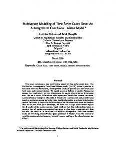
Figure 1: Autocorrelation Function of deseasonalized absolute price tick change (sample: June 2013-Dec. 2013 - 5 Minutes time interval) 175

19

0.4

ACF

0.3 0.2 0.1 0.0 1 20 42 64 86 111 139 167 195 Lag

Figure 2: Autocorrelation Function of INAR(1) innovations (sample: June 2013-Dec. 2013 - 5 Minutes time interval) 176

4

Conclusion

177

This paper has stressed that integer processes may suite well intraday

178

data analysis. It introduces an integer auto-regressive moving average pro-

179

cess (INARMA) with integer GARCH (INGARCH) innovations. Conditional

180

and unconditional mean and variance of the INARAMA(1,1)INGARCH(1,1)

181

process, as well as their auto-covariance were computed. The paper has also

182

presented an integer autoregressive process (INAR) with integer GARCH

183

innovations. As with the INARMA(1,1)-INGARCH(1,1) process, the condi-

184

tional moments of the INAR(1)-INGARCH(1,1) was shown to also depend

185

on past innovations. Both processes were estimated by maximizing the as-

186

sociated conditional log-likelihood of the Poisson p.m.f. 20

0.4

ACF

0.3

0.2

0.1

0.0 1 18 38 58 78 98 121 147 173 199 Lag

Figure 3: Autocorrelation Function of INAR(1)-INGARCH(1,1) innovations (sample: June 2013-Dec. 2013 - 5 Minutes time interval) 187

In the case of the ARMA-GARCH, the innovation process represents the

188

randomness of the price process. While with the INARMA-INGARCH there

189

are more than one sources of randomness, i.e.: the innovation process and

190

the number of thinning operators. Unlike its continuous time counterpart,

191

the structure of the INARMA-INGARCH process is not divided into the

192

usual deterministic and stochastic component and is only conditionally linear.

193

In application to intraday asset prices, it represents a birth-death process

194

for new information arrivals and departures and therefor an opportunity to

195

better describe intraday price variations. The model can be extended to allow

196

for an unconditional over-dispersion (e.g.: negative-binomial distribution) or

21

0.4

ACF

0.3

0.2

0.1

0.0 1 18 38 58 78 98 121 147 173 199 Lag

Figure 4: Autocorrelation Function of INARMA(1,1)-INGARCH(1,1) innovations (sample: June 2013-Dec. 2013 - 5 Minutes time interval) 197

by considering more generalized thinning operators (e.g.: random coefficient

198

thinning).

199

Reported results indicate that, relative to the ARMA(1,1)-GARCH(1,1),

200

integer-based models may provide a more accurate point forecast of future

201

realizations of intraday absolute tick price change. These results also suggests

202

that the INAR(1)-INGARCH(1,1), a simpler process, may be also reliable for

203

forecasting absolute tick price changes. However, since the GARCH process

204

is an ARMA process of squared returns, the INARMA-INGARCH process

205

may be theoretically more appropriate.

22

206

There are some caveats to model absolute tick size changes. To begin, the

207

Poisson (as well as the Negative Binomial distribution) can only consider non-

208

negative realizations and innovations. Restricting the analysis to absolute

209

values makes it difficult to be used to model the VaR. For futures (such as

210

the E-mini S&P 500) describing intraday asset price dynamics accurately is

211

important for hedging since the variance (as well as the covariance) is required

212

to compute the optimal hedge ratio. Financial theory has not, however, been

213

concerned with integer process models, especially when considering hedging

214

and optimal assets allocation. Application of the models considered here

215

provide such an opportunity. Further, the need to generalize the model to

216

negative realizations as well as adapting intraday processes to their financial

217

applications requires further research.

23

218

References

219

References

220

AA Alzaid and M Al-Osh. An integer-valued pth-order autoregressive struc-

221

ture (inar (p)) process. Journal of Applied Probability, pages 314–324,

222

1990.

223

Torben G Andersen and Tim Bollerslev. Intraday periodicity and volatility

224

persistence in financial markets. Journal of empirical finance, 4(2):115–

225

158, 1997.

226

227

228

229

Tim Bollerslev. Generalized autoregressive conditional heteroskedasticity. Journal of econometrics, 31(3):307–327, 1986. Peter F Christoffersen. Elements of financial risk management. Academic Press, 2011.

230

Robert F Engle and Jeffrey R Russell. Autoregressive conditional duration:

231

a new model for irregularly spaced transaction data. Econometrica, pages

232

1127–1162, 1998.

233

Robert F Engle and Magdalena E Sokalska. Forecasting intraday volatility in

234

the us equity market. multiplicative component garch. Journal of Financial

235

Econometrics, 10(1):54–83, 2012.

24

236

237

238

239

240

241

Ren´e Ferland, Alain Latour, and Driss Oraichi. Integer-valued garch process. Journal of Time Series Analysis, 27(6):923–942, 2006. Konstantinos Fokianos. Some recent progress in count time series. Statistics, 45(1):49–58, 2011. Christian Francq and Jean-Michel Zakoian. Mod`eles GARCH: structure, inf´erence statistique et applications financi`eres. Economica, 2009.

242

Eric Ghysels and Joanna Jasiak. Garch for irregularly spaced financial data:

243

the acd-garch model. Studies in Nonlinear Dynamics & Econometrics,

244

2(4), 1998.

245

Harry Joe. Time series models with univariate margins in the convolution-

246

closed infinitely divisible class. Journal of Applied Probability, pages 664–

247

677, 1996.

248

249

250

251

252

253

254

Hee-Young Kim and Yousung Park. A non-stationary integer-valued autoregressive model. Statistical papers, 49(3):485–502, 2008. Ed McKenzie. Some arma models for dependent sequences of poisson counts. Advances in Applied Probability, pages 822–835, 1988. Peter Neal and T Subba Rao. Mcmc for integer-valued arma processes. Journal of Time Series Analysis, 28(1):92–110, 2007. Jeffrey R Russell and Robert F Engle. A discrete-state continuous-time model

25

255

of financial transactions prices and times. Journal of Business &

256

Economic Statistics, 23(2), 2005.

257

258

259

M. Scotto Turkman, Kamil Feridun and Patr´ıcia de Zea Bermudez. NonLinear Time Series. Springer, 2014. Christian H Weiß. Serial dependence and regression of poisson inarma mod-

260

els.

261

2008a.

262

263

264

265

Journal of Statistical Planning and Inference, 138(10):2975–2990,

Christian H Weiß. Thinning operations for modeling time series of counts—a survey. AStA Advances in Statistical Analysis, 92(3):319–341, 2008b. Christian H Weiß. A poisson inar (1) model with serially dependent innovations. Metrika, pages 1–23, 2015.

266

Hai-Yan Xu, Min Xie, Thong Ngee Goh, and Xiuju Fu. A model for integer-

267

valued time series with conditional overdispersion. Computational Statis-

268

tics & Data Analysis, 56(12):4229–4242, 2012.

269

Haitao Zheng, Ishwar V Basawa, and Somnath Datta. First-order random

270

coefficient integer-valued autoregressive processes. Journal of Statistical

271

Planning and Inference, 137(1):212–229, 2007.

26

272

A

Proof of proposition 1

The unconditional mean is obtained by taking the expectation of the conditional mean in equation (11), i.e.:

E [E [Yt,i |Ωt,i−1 ]] = ρE [Yt,i−1 ] + θE [t,i−1 ] + E [λt,i ]

(1)

Where, the unconditional mean of the innovation process (t,i ) is similar to the unconditional mean of the innovation process in a simple GARCH pro¯ = E [λt,i ], we obtain the unconditional mean of the innovation cess. Writing λ process, i.e.: ¯= E [t,i ] = λ

ω 1−α−β

(2)

Substituting in equation (A.1), the unconditional mean of Yt,i is: ω ¯1 − θ = E [Yt,i ] = µY = λ 1−ρ (1 − ρ)(1 − α − β)

(3)

To compute the unconditional variance of the INARMA(1,1)-INGARCH(1,1) we first consider the unconditional variance of the innovation process. Using the law of total variance, the unconditional variance of t,i is: V [t,i ] = E [Vt,i−1 (t,i )] + V [Et,i−1 (t,i )] (4) ¯ + V [λt,i ] =λ

27

Using the law of total covariance on Cov (t,i , λt,i ), the variance of the autoregressive intensity process (λt,i ) is given below: V [λt,i ] = α2 V [t,i−1 ] + β 2 V [λt,i−1 ] + 2αβCov (t,i−1 , λt,i−1 )
¯ + V [λt,i ] + β 2 V [λt,i−1 ] + 2αβV [λt,i−1 ] = α2 λ ¯ α2 λ = = σλ2 1 − (α + β)2

(5)

Applying the law of total variance again on Yt,i , we obtain:

V [Yt,i ] = E [Vt,i−1 (Yt,i )] + V [Et,i−1 (Yt,i )]

(6)

Plug-in the conditional moments in equation (11) into equation (A.6) yields:

¯ + θ(1 − θ)λ ¯ + ρ2 V [Yt,i ] + θ2 (λ ¯ + σ2 ) + σ2 V [Yt,i ] = ρ(1 − θ)λ λ λ + 2ρθCov (t,i , Yt,i ) + 2ρCov (λt,i , Yt,i−1 ) + 2θCov (t,i−1 , λt,i )

28

(7)

We use again the law of total covariance and the law of iterated expectations to calculate the covariance terms. ¯ + σ2 Cov (t,i , Yt,i ) = ρCov (t,i , Yt,i−1 ) − θCov (t,i , t,i−1 ) + λ λ Where : (8)

Cov (t,i , Yt,i−1 ) = Cov (λt,i , Yt,i ) Cov (t,i , t,i−1 ) = Cov (t,i−1 , λt,i ) ¯ + σ2 ∴ Cov (t,i , Yt,i ) = ρCov (λt,i , Yt,i−1 ) − θCov (t, i − 1, λt,i ) + λ λ Similarly we also obtain: Cov (Yt,i−1 , λt,i ) = αCov (t, i, Yt,i )

(9) ¯ + (α + β)σ 2 Cov (t,i−1 , λt,i ) = αλ λ 273

Plug-in equation (A.9) in equation (A.8) and then in equation (A.7) we obtain

274

the unconditional variance (equation 13) in proposition 1.

275

B

Proof of proposition 2

The auto covariance function is computed reclusively. Note, the covariance terms in equation (14) are computed using the law total covariance and law of iterated expectations. To start, the auto-covariance of order one is:

Cov (Yt,i , Yt,i−1 ) = ρσY2 − θCov (t,i , Yt,i ) + Cov (t,i , Yt,i−1 )

29

(10)

And the auto-covariance of order two is: Cov (Yt,i , Yt,i−2 ) = ρCov (Yt,i , Yt,i−1 ) − θCov (t,i , Yt,i−1 ) (11) + Cov (t,i , Yt,i−2 ) Then plugin equation (B.1) into (B.2) yields: Cov (Yt,i , Yt,i−2 ) = ρ2 σY2 − θρCov (Yt,i , t,i ) + (ρ − θ)Cov (t,i , Yt,i−1 ) + Cov (t,i , Yt,i−2 ) 276

Repeating this step j times yields equation (14) in proposition 2.

30

(12)