Introducing Complex Automata for Modelling Multi-Scale Complex Systems Alfons G. Hoekstra(1), Bastien Chopard(2), Pat Lawford(3), Rod Hose(3), Manfred Krafczyk(4), Joerg Bernsdorf(5) (1) Section Computational Science, University of Amsterdam, The Netherlands,
[email protected],l corresponding author (2) University of Geneva, Switzerland,
[email protected] (3) University of Sheffield, UK, {p.lawford, d.r.hose}@sheffield.ac.uk (4) Technical University Braunschweig, Germany,
[email protected] (5) C&C Research Laboratories, NEC Europe Ltd.,
[email protected]
Abstract We introduce Complex Automata, a generic methodology to model multi-scale complex systems. A Complex Automaton is a scalable hierarchical aggregation of Cellular Automata and agent-based models, each modelling components of the Complex System. The components represent a sub-system operating on its typical spatial and temporal scales. The concept of a scale map is introduced to identify components and to define appropriate couplings. For two case studies a high level description in terms of a Complex Automaton will be presented.
1
Introduction
Complex systems are composed of many entities whose mutual interactions produce emergent and collective behaviours. Computer simulations and rule-based modelling are often the only effective methodologies available to describe complex systems and understand or control their behaviour. Cellular Automata and agent-based models are often presented as the ideal mathematical abstraction of a complex system. However, as many complex systems encompass several spatial and temporal scales, as well as several types of elementary components, a single, homogeneous model cannot in general describe them. In this paper we discuss multi-scale modelling of complex systems that are made of components that act on multiple, possibly overlapping time and length scales. We introduce a new approach where we take Cellular Automata (CA) [1] and agent-based models [2] as basic modelling blocks to create a hierarchical aggregation of such basic models, leading to what we call a Complex Automaton. In Complex Automata all spatial and temporal scales may be coupled and/or treated on the same footing. The Complex Automaton framework addresses the issue of subsystem coupling using a scale splitting methodology to discover effective simulation strategies. In this contribution we introduce the concept of Complex Automata and formulate a methodology to specify a Complex Automaton. Next we present two case studies, being the modelling of coral growth and of snow deposition and erosion, and we show how these models are captured within the Complex Automata framework.
2
Complex Automata
A Complex automaton is a generalization of Cellular Automata and agent-based models. It is a set of autonomous automata, each having its specific rules of evolution. These entities can be spatially coupled to similar automata or to other types of automata with completely different behaviour. A given automaton itself may again be composed of a set of automata, thus introducing the concept of hierarchical coupling.
Page 1 of 6
Introducing Complex Automata
ECCS’06
A private clock governs the behaviour of each automaton. A clock may be shared, in a synchronous way, by several automata with the same dynamical time scale, whilst others have their own private clocks and update their states asynchronously. Automata are coupled by sharing information through their input and output ports. The shared information may be detailed temporally and/or spatially resolved signals, lumped data, or some mix form. In the first case automata are typically connected, through their boundaries for example, and exchange detailed information. In case of lumped data it may be that one automaton results in data that is an input parameter to another automaton (e.g. a simulation conducted at a micro length scale that results in parameters to be used in a macroscopic simulation). The details of the shared information (resolved versus lumped) and the details of the dynamics of exchanging of the information (synchronous versus asynchronous, time-driven versus event-driven, etc.) will dictate the mechanism of model coupling. The time coupling in Complex Automata can be viewed as data driven processes, where automata may behave in an eager (that is, immediately respond to input changes) or in a lazy way (that is, only react when output is required). Model coupling requires that common quantities be built at the interface between interacting sub-systems. These quantities reflect how the emerging properties of one process affect the others, by imposing specific boundary conditions in space and time or by defining some values of parameters. Most of the time, the identification of the quantities that will govern the coupling first implies a good knowledge of all subsystems independently and the different space-time regimes that they may settle in. When taken individually, all subsystems are characterised by their internal dynamics, their boundary condition and possibly global parameters that reflect some coupling with the environment. When the coupling is considered, the boundary conditions are shared amongst two or more parts and are no longer a controlled region. The challenge in coupling Complex Automata is to adopt numerical techniques where possible and develop new approaches where required. An example of non-standard coupling is the case where a Finite-Element Code or a Lattice-Boltzmann Automaton (both floating-point based) have to be coupled to an integer based CA [3]. Here one must achieve mapping of the primary variables via ensemble averaging while keeping the accuracy of the float-state CA in spite of the internal noise typically present in classical integer CA. The selection of scales may be based on prior scientific knowledge, or could be inferred from detailed studies of sub-systems. Scale separation naturally builds up as an emergent property of the system. A scale map is defined with the horizontal axis coding for temporal scales and the vertical axis coding for spatial scales. Each subsystem occupies a certain area on this map. Fig. 1 shows an example of such a scale map, in which three subsystems have been identified. Subsystem 1 operates on small spatial scales, and short time scales, process 2 at intermediate scales, and process three at large scales. This could e.g. be processes operating at the micro-, meso-, and macro scale. As a more specific example, in the coral growth model (see section 3.1 for details), two subsystems would be the growing coral and the hydrodynamics, with both systems on comparable spatial scales, but widely separated in the temporal scale. On the other hand, turbulence would be considered to fill a tilted line across many orders of magnitude in the spatial and temporal scales (i.e. a continuum of scales).
Page 2 of 6
Introducing Complex Automata
ECCS’06
spatial scale 3 lumped parameter coupling
spatially and temporally resolved coupling 2
1
temporal scale Figure 1: A scale map, showing three sub-systems and their mutual couplings.
After identifying all subsystems and placing them on the scale map, coupling between subsystems is then represented by directed edges on the map. In Fig. 1 process 1 is coupled with 3 through a lumped parameter, and there is no feedback from process 3 back to process 1. Process 2 and 3 are coupled through detailed spatially and temporally resolved signals, so they would typically share a boundary and synchronously exchange information. The distance between subsystems on the map indicates which model embedding method to use to simulate the overall system. In the worst case, one is forced to use the smallest scales everywhere, probably resulting in intractable simulations. On the other hand, if the subsystems are well separated and the smallest scale subsystems are in equilibrium, then they can be solved separately, although infrequent (possibly event-driven) feedback between the subsystems will still be required.
3
Two Case Studies
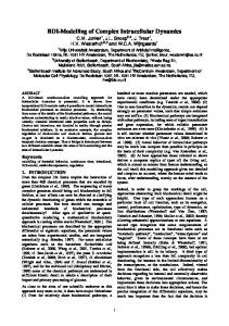
In previous work we have gained experience with modelling complex systems showing emergent behaviour, but we did not explicitly employ the ideas behind Complex Automata. In this section we present two examples, and recast them in terms of Complex Automata. We show how the models can be decomposed, how the subsystems are positioned on the scale map, and how their coupling is. 3.1 Coral Growth The growth of branching corals is modelled, with the aim to understand the influence of abiotic factors (transport of nutrients by flow and diffusion) on the morphology. This is work performed under the supervision of Dr. Jaap Kaandorp, and for biological context and background we refer to his recent book. [4] The resulting morphology, typically a complex branching structure, is the emergent property of the model. The growth is governed by influx of nutrients, which are transported to the coral by an advection – diffusion mechanism. Three processes can be distinguished: (1) growth of the coral; (2) flow of water around the coral; and (3) advection – diffusion of nutrients. All three processes happen at the same length scale, which is a typical diameter of a branch of the coral, or a typical distance between the branches, in all cases O(cm). On this length scale, the growth itself is an extremely slow process, for a typical species that was studied growth was O(cm/year). Both the flow and advection – diffusion are much faster, on the scale of seconds and minutes (diffusion time scale) respectively. For details of the model and discussions on the scale separation we refer to [5, 6, 7]. Figure 2 shows the scale map for the Coral growth model. We distinguish the three subsystems, qualitatively drawn at their scales. Moreover, the couplings are shown. The boundary condition for the flow is provided by the coral surface. The flow fields are spatially resolved input for the advection – diffusion, in which the coral surface again provides a
Page 3 of 6
Introducing Complex Automata
ECCS’06
boundary condition. Finally, the advection – diffusion solver provides flux of nutrients at the coral surface, with is a spatially resolved input for the growth model. boundary condition; velocity zero at coral surface
spatial scale
Flow
flow field
Advection Diffusion
flux of nutrients at coral surface
growth
boundary condition; coral surface a sink for nutrients
temporal scale Figure 2: Scale map for the Coral growth model
The execution of the full model is a synchronous iteration over the three subsystems. First, the flow is computed, next the nutrients concentration is computed, and finally a growth step is performed. This is typically iterated over some 100 growth steps. The flow and advection – diffusion model are both based on Lattice Boltzmann Cellular Automata, the growth model can be an accretion or aggregation model. For details we refer to [8] and references therein. In Fig. 3 we show a range of resulting growth forms, dependent on the surrounding fluid flow. In sheltered conditions (i.e. low flow velocities, diffusion dominates) strong branching structures our found, whereas in high flow conditions the coral becomes more compact. For certain species of coral this is also observed in reality. [see e.g. 4]
Figure 3: A range of simulated morphologies, depending on the Peclet number. Left is for low Peclet number (i.e. diffusion dominates) and right for high Peclet number (i.e. flow dominates).
3.2 Snow Deposition Snow (or sand) transport, deposition and erosion due to the action of wind has been simulated [9,10] in a way that can be cast in the proposed complex automata framework. The wind component is described by a Lattice Boltzmann model and is coupled to a multi-particle CA [11 representing the snow particles. The fluid model spans several space and time scales as it must capture the flow pattern at the scale of the full simulation (e.g. the average wind speed) as well as the perturbations caused by small obstacles (e.g a fence) and the changes in boundary conditions due to the accumulation of snow that occurs during the simulation. The grid spacing and time step are chosen so as to resolve with the desired accuracy the shape of the obstacles and the deposition profile. Larger scale features will build up as an emergent property. Note that smaller scales, which should be present as the wind may have a turbulent nature, are taken care of with a sub-grid model. This can be seen as an implicit coupling of each wind cell with a subsystem, through the shear stress and a lumped resulting viscosity. Snow particles are described as point-particles. They are transported as passive scalars by the combined action of wind and a sedimentation speed. Snow particles that reach a deposition
Page 4 of 6
Introducing Complex Automata
ECCS’06
layer pile up on top of it. When enough of them have accumulated in a given spatial region, they solidify and form a new part of the deposition layer. This automatically causes a change for the wind boundary conditions. Erosion is however possible: if the local shear stress is large enough, snow particles at rest can be picked up and transported again by the wind. From a modelling point of view, the snow particles are described by a multi-particle CA whose cell size matches that of a wind cell and spans the same spatial area. Thus, the coupling between the two systems is implemented between the corresponding cells. This also means that the snow cells have a size which is imposed by the chosen wind resolution. Thus, as snow particles have a typical diameter, the maximum number of snow particles that can exist in a cell before it solidifies as a patch of the deposition layer can be adjusted according to the chosen scale. In other words, a bit like the turbulent sub-grid model, the small scale features of snow particles are described by a simplified dynamics at the level of each cell. Phenomena at a larger scale than the cell size naturally build as the result of the interaction map shown in fig. 4. Figure 5 shows the result of a simulation of snow transport, erosion and deposition in presence of a fence with a bottom clearance. We can observe the formation of a small deposit upstream and a large one downstream. The ratio of the deposition length to the fence height agrees with field observations. We refer the reader to ref. [9] for more details.
spatial scale flow Flow transport transport
erosion Erosion
deposition deposition
temporal scale
Figure 4: Scale map for the snow deposition and erosion model
Figure 5: Four snapshots during the simulation. Time increases from left to right and top to bottom. The yellow region shows the snow deposit whereas the white pixels indicate airborne snow particles.
4
Discussion & Conclusions
Multi-scale modelling and simulation attracts a growing research community, and many different solutions have been proposed. Typically such solutions are driven by a specific
Page 5 of 6
Introducing Complex Automata
ECCS’06
application domain, and a large diversity of models and simulation environments are then coupled. A good example of such approach is the Japanese OCTA project. [12] Our approach is different. We restrict ourselves to two model paradigms, generally acknowledged for their capability of modelling complex systems, and then use those to derive a generic modelling approach for multi-scale complex systems. Within the EU funded COAST project we will further develop Complex Automata by defining a mathematical framework, developing a generic simulation environment, and validating the approach by considering an application from biomedicine. Modelling biomedical systems is a very challenging problem with a strong impact on society. The inherent complexity of biomedical systems is now beginning to be appreciated fully: they are multi-scale – multi-science systems, covering a range of phenomena from molecular and cellular biology, via physics and medicine, to engineering and crossing many orders of magnitude in temporal and spatial scales. [13] To be more specific, we will address the adverse vessel wall remodelling (re-stenosis), which occurs in some patients after placement of a metal frame (stent) within the artery lumen to expand and support the vessel at the site of a stenosis. This phenomenon of in-stent re-stenosis involves several biological and physical subprocesses, spanning a wide range of spatial and temporal scales. To model restenosis, drug release, and inhibition of re stenosis we need to include a representation of physical processes (haemodynamics, convection and diffusion, species transport, tissue stresses), chemical processes (drug uptake, metabolism and reaction models), and biological processes (cell signalling, cell cycle/division, cellular response to physical and chemical signals), each with their own spatial and temporal scales, and their mutual coupling. By casting these processes in Cellular Automata (most of the physics) and agent based models (most biological processes) and hierarchically coupling them according to the Complex Automata framework, we expect to be able to simulate the process of in-stent re-stenosis. This will be investigated by validating the simulations against in-vivo data.
5
Acknowledgements
This work is supported by the EU 6th framework program, through the IST-FET initiative on Complex Systems, contract number 033664 (COAST).
6
1
References
Andrew Ilachinski, Cellular Automata: A Discrete Universe, World Scientific Publishing (Singapore), 2001.
2 Michael Wooldridg, Introduction to MultiAgent Systems, John Wiley & Sons, 2002. 3 M. Krafczyk, “Gittergasmethoden”, PhD thesis, Chair for Information Processing and Numerical Methods, 4 5 6 7 8 9 10 11 12 13
University of Dortmund, 1994 J.A. Kaandorp and J.E. Kübler: The algorithmic beauty of seaweeds, sponges and corals, Springer-Verlag (Heidelberg, New York) 2001. R.M.H. Merks; A.G. Hoekstra; J.A. Kaandorp and P.M.A. Sloot, “Models of coral growth: Spontaneous branching, compactification and the Laplacian growth assumption”, J. Theor. Biol. 224, 153-166, 2003. R.M.H. Merks; A.G. Hoekstra; J.A. Kaandorp and P.M.A. Sloot, “Diffusion Limited Growth In Laminar Flows”, Int. J. Mod. Phys. C 14, 1171-1182, 2003. R.M.H. Merks; A.G. Hoekstra; J.A. Kaandorp and P.M.A. Sloot, “Polyp oriented modelling of coral growth”, J. Theor. Biol. 228, 559-576, 2004. R.M.H. Merks; A.G. Hoekstra; J.A. Kaandorp; P.M.A. Sloot and P. Hogeweg, “Problem-Solving Environments for Biological Morphogenesis”, Comput. Sci. Eng 8, 61-72, 2006. A. Masselot and B. Chopard, “A lattice Boltzmann model for particle transport and deposition”, Europhys. Lett. 42, 259 - 264, 1998. Alexandre Dupuis and Bastien Chopard, “Lattice gas modeling of scour formation under submarine pipelines”, J. Comp. Phys. 178, 161 - 174, 2002. B. Chopard and M. Droz, Cellular automata modeling of physical systems, Cambrige University Press, 1998 www.octa.jp S.W. Smye, R.H. Clayton, “Mathematical modelling for the new millennium: medicine by numbers”, Medical Engineering and Physics 24, 565-574, 2002.
Page 6 of 6