Introduction. - CiteSeerX

ON NEWHOUSE REGIONS WITH INFINITELY MANY STABLE AND UNSTABLE INVARIANT TORI S. V. Gonchenko, L. P. Shilnikov and O. V. Stenkin Research Institute for Applied Mathematics and Cybernetics, Nizhny Novgorod, Russia

Abstract We consider two-dimensional dieomorphisms close to a dieomorphism with a nontransversal heteroclinic cycle composed from several saddle hyperbolic xed points and heteroclinic orbits, at least one of wich is nontransversal. We show that if the cycle has at least two xed points such that the Jacobian of one of them is less and of another is greater than one, then near such a dieomorphism Newhouse regions exist in which dieomorphisms having simultaneously in nitely many saddle, stable and completely unstable periodic orbits as well as stable and unstable periodic close invariant curves are dense. This assertion is also true for two parameter families in general position.

Introduction. As is well known, multidimensional structurally unstable systems can form regions in the space of smooth dynamical systems. Regions where there is a dense set of systems with saddle periodic orbits having tangencies of their stable and unstable manifolds along homoclinic orbits are among the most important examples of such systems. Such regions were discovered by Newhouse [1] for the case of two-dimensional dieomorphisms close to a dieomorphism satisfying the following conditions: (i) the saddle value   j j of a xed point O is dierent from 1 (where  and are multipliers of O, 0 < jj < 1 < j j); (ii) a tangency of the stable W s (O) and unstable manifolds W u (O) is quadratic. Later, this Newhouse result was extended onto the multidimensional case in [2,3,4]. Moreover, the existence of regions of the structural instability was established in the case of generic (in general position) nite-parameter families [2]. Naturally, such regions, both in the space of dynamical systems and in the parameter space, have been called as Newhouse regions. One of important peculiarities of the orbit behavior for systems in Newhouse regions is the coexistence of hyperbolic orbits of various types. For instance, two-dimensional dieomorphisms having simultaneously in nitely

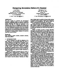
Figure 1: Dieomorphism with non-transversal heteroclinic cycle consisting of a) several saddle xed points, b) two saddle xed points (the simplest cycle). many saddle and stable (if  < 1) or completely unstable (if  > 1) periodic orbits are dense in Newhouse regions; in the multidimensional case, saddle periodic orbits with dierent dimensions of stable manifolds can coexist [5]. Another principle peculiarity of Newhouse regions is the existence of in nitely degenerate systems. In particular, systems with in nitely many arbitrary degenerate periodic orbits as well as systems with in nitely many homoclinic tangencies of any order are dense in Newhouse regions [6{9]. In the case of two-dimensional dieomorphisms close to a dieomorphism with a homoclinic tangency to a saddle xed point with  6= 1, periodic orbits of dieomorphisms from Newhouse regions can have only one multiplier equal to one in the absolute value. In the multidimensional case periodic orbits can have several multipliers on the unit circle (see [5,8]). Newhouse regions also exist near a dieomorphism with a nontransversal heteroclinic cycle consisting of several saddle xed (periodic) points and heteroclinic orbits (Fig.1a). In the main case (codimension one) the heteroclinic cycle contains only one nontransversal heteroclinic orbit with a quadratic tangency of corresponding stable and unstable manifolds and, besides, the saddle values of all xed points of the cycle are dierent from one. The case where all saddle values are either less or greater than one does not dier principally from a homoclinic case. However, if the cycle has at least two xed points such that the saddle value of one of them is less and of another is greater than one, then a new phenomenon arises [10]: near such a dieomorphism Newhouse regions exist in which dieomorphisms having simultaneously in nitely many saddle, stable and completely unstable periodic orbits are dense. This assertion is also true for one parameter families in general position [10]. Moreover, one can

point out one more characteristic peculiarity of the corresponding Newhouse intervals. Namely, in such an interval there are dense values of a parameter within such an interval when a dieomorphism of a family has a heteroclinic cycle "of an initial type": it contains the same saddle xed points which are in the initial cycle, close transverse heteroclinic orbits and new (multi-round) heteroclinic orbit with a quadratic tangency of stable and unstable manifolds. In this situation, it is naturally to speak about Newhouse regions (intervals) with heteroclinic tangencies. Note that in these regions dieomorphisms with homoclinic tangencies are also dense and, consequently, dieomorphisms with above mentioned degenerate periodic and homoclinic orbits are dense . However, since contraction and expansion of areas are observed near the cycle, one can expect that periodic orbits of a "neutral type" can exist in such Newhouse regions, for example, periodic orbits with two multipliers on the unit circle. In this case we can hope that dieomorphisms with in nitely many closed invariant curves will be dense in these Newhouse regions. This paper is devoted to solving this problem.

1 Main results. We study bifurcations of periodic orbits of two-dimensional dieomorphisms close to a dieomorphism with a nontransversal heteroclinic cycle. In general case, such a cycle consists of several saddle (hyperbolic) periodic orbits, O1 ; :::; On, and heteroclinic orbits, ?1;2 ; :::; ?n?1;n and ?n;1 ; such that ?i;i+1  W u (Oi) \ W s(Oi+1 ) ; i = 1; :::; n ? 1; and ?n;1  W u (On) \ W s(O1) ; i = 1; :::; n ? 1; and, besides, tangent heteroclinic orbits exist among pointed out ones (Fig.1a). We consider the case when at least two orbits among O1; :::; On are such that the saddle value of one of them is less and of another is greater than one. We will call such a cycle the mixed type nontransversal heteroclinic cycle. It was established in [10] that Newhouse regions of three types can exist near dieomorphisms with such type cycles. We note especially, that Newhouse regions of the rst type exist always and, moreover, both dieomorphisms having homoclinic tangencies to any point from O1; :::; On and dieomorphisms having simultaneously in nitely many saddle, stable and completely unstable periodic orbits are dense in these regions.1 . Besides, when the dieoomorphism has in nitely many stable and completely unstable, the closure of the sets of these orbits is nonempty: in any case, it contains orbits O1 ; :::; On. Note that Newhouse regions of the second and third types, in contrast to these of the rst type, do not contain dieomorphisms with any homoclinic orbits to some saddles from O1 ; :::; O ; and Newhouse regions of the third type have no dieomorphisms either with stable either with completely unstable periodic orbits (see for details in [10]) 1

n

In this paper we continue to study dynamical properties of dieomorphisms from Newhouse regions of the rst type. Our main result is the following

Theorem A. In any Newhouse region of the rst type there is a dense set

of dieomorphisms having in nitely many stable and in nitely many unstable closed invariant curves, and, moreover, orbits O1; :::; On belong both to the closure of the set of the stable invariant curves and to the closure of the set of the unstable closed invariant curves.

Theorem A characterizes dynamical properties of systems from the Newhouse regions as open regions in the space of two-dimensional dieomorphisms.2 Certainly, the question on the existence of analogous Newhouse regions in the parameter space for general nite parameter unfoldings is more interesting. Note that the existence of Newhouse intervals of the rst type was proved in [10] for one-parameter families of general position containing (at zero value of a parameter) a dieomorphism with a mixed type nontransversal heteroclinic cycle. In the simplest case, such a cycle has two xed saddle (hyperbolic) points O1 and O2 and two heteroclinic orbits ?12  W u (O1) \ W s (O2) and ?21  W u (O2)\W s (O1) such that W u (O1) and W s (O2) intersect transversally at the points of orbit ?12 and W u (O2) and W s (O1) have a quadratic tangency at the points of orbit ?21 (Fig.1b). Let f0 be such a C r -dieomorphism (r  3) with the simplest mixed type nontransversal heteroclinic cycle (i.e. one of the saddle values of points O1 or O2 is less and the other is greater than one), and let f1 be a one parameter C r -family of general position (where, for example, 1 is a parameter governing with the splitting manifolds W u (O2(1 )) and W s (O1(1 )). It was established in [10] that in the interval I = (?"; ") for any " > 0 there is a countable set of intervals j  I of values of 1 such that j ! 0 as j ! 1 and 1) for any 1 2 j dieomorphism f1 has a nontrivial hyperbolic subset (including in nitely many saddle periodic orbits and points O1 and O2); 2) in j there are dense values of 1 at which dieomorphism f1 has in nitely many stable and in nitely many completely unstable periodic orbits whose closure contains points O1 and O2; 3) in j there are dense values of 1 , 1 = 1 , at which dieomorphism f1 has a simplest nontransversal cycle consisting of orbits O1(1 ), O2 (1), ?12 (1 ) and of a nontransversal heteroclinic orbit ?j21 (1 ) in whose points manifolds W u (O2(1 )) and W s (O1(1 )) have a quadratic tangency and the parameter 1 ? 1 split monotonically this tangency. Note that dieomorphisms of theorem A form residual sets in the corresponding Newhouse regions from the space of two-dimensional C -dieomorphisms with C -topology where r  3. In this sense, such dieomorphisms are generic (typical) 2

r

r

In the present paper we consider two-parameter families and study bifurcations of appearance of closed invariant curves. Let now f0 be a C r smooth, r  5, two-dimensional dieomorphism with the simplest mixed type nontransversal heteroclinic cycle. Consider a two-parameter family f where  = (1 ; 2) and the dieomorphism of the family coincides with f0 at 1 = 0; 2 = 0. As 1 we consider a parameter governing with the splitting manifolds W u (O2) and W s (O1). As 2 we choose a parameter which controls the change of the saddle values 1 and 2 of points O1() ¨ O2 ().

Theorem B. On the parameter plane (1; 2) in any neighbourhood of the origin there exist regions
i in which values of  are dense such that diffeomorphism f has simultaneously in nitely many stable and unstable closed invariant curves. The closure of the set of stable closed invariant curves contains points O1 () and O2 (), the same is true for the closure of the set of unstable closed invariant curves. Thus, combining results of [10] and theorems A and B we prove the existence of two-dimensional dieomorphisms with "totally mixed dynamics" in the sense that such dieomorphisms have simultaneously in nitely many hyperbolic periodic orbits of all kinds and in nitely many stable and unstable closed invariant curves and, besides, the sets of orbits of dierent types are not separated from each other. We consider C r -smooth, (r  5), two-dimensional dieomorphism f0 having the simplest nontransversal heteroclinic cycle. That is, f0 has two hyperbolic saddle xed points O1 and O2 whose the invariant manifolds behave as follows: W u (O1 ) and W s (O2) intersect transversally at the points of a heteroclinic orbit ?12 and W u (O2) and W s (O1) have a quadratic tangency at the points of a heteroclinic orbit ?21 . The heteroclinic cycle C consists of the orbits O1 ; O2; ?12 and ?21 . Let i and i be multipliers of the point Oi where ji j < 1; j ij > 1; i = 1; 2 . Denote i the saddle value of Oi , i.e. i = ji i j. We will consider the case where either 1 < 1 < 2 or 2 < 1 < 1 . Thus, the cycle under consideration is the simplest mixed type nontransversal heteroclinic cycle. Dieomorphisms which are C r -close to f0 and have a close nontransversal heteroclinic cycle form a codimension one bifurcation surface H in the space of C r -dieomorphisms. When studying bifurcations of such dieomorphisms one needs, rst of all, to consider one-parameter general unfoldings, as was considered in [10]. But, keeping in mind that our main problem is to study bifurcations of appearance of closed invariant curves, we will consider two parameter families f of general position, where  = (1 ; 2) and the dieomorphism of the family coincides with f0 at 1 = 0; 2 = 0. As

one of the governing parameters, 1 , we choose a parameter of splitting manifolds W u (O2) and W s (O1). As another governing parameter, 2 , we choose a parameter which controls the saddle values 2 and 1 of points O1 () and O2 (). Consider the following positive-valued functional 2  (f ) = ? ln ln 1 We will take as 2 such a parameter that @ (f ) 6= 0 ;  (f ) = 0 :

@2

2 0

In particular, we take directly

2 =  (f ) ?  (f0)

(1)

The sense of this choice will be clear below (see section 4). Contents of the paper. In x 2 general properties of dieomorphisms with the simplest nontransversal heteroclinic cycles are considered; the rst return map are constructed and brought, by rescaling coordinates and parameters, to the generalized Henon map. In x 3 bifurcations of single-round periodic orbits are studied. In x 4 theorem A and B are proved.

2 Construction of rst return maps. Let U be a small xed neighbourhood of the cycle C . It is a union of two discs U1 and U2 containing points O1 and O2 and of a number of discs containing points of orbits ?12 and ?21 which lie outside U1 and U2. Denote by T0l (), l = 1; 2; the restriction of f onto Ul , i.e. T0l()  f U . We will call maps T01() and T02() the local maps. It is well known [11,12] that one can introduce such C r?1 -coordinates (xl ; yl) on Ul that T0l() is written in the form xl = l()xl + fl (xl; yl; )x2l yl ; (2) yl = l()yl + gl(xl; yl; )xlyl2 ; l

where the right sides of (2) are C r?1 (in coordinates and parameters). Then, at all suciently small , the point Ol() has coordinates xl = 0; yl = 0 and the s (Ol ()) and W u (Ol()) are yl = 0 and xl = 0 , respectively. equations of Wloc loc Consider again the dieomorphism f0 . The point O1 is -limit for ?12 and ! -limit for ?21 ; the point O2 is -limit for ?21 and ! -limit for ?12 . Hence, countable sets of heteroclinic points (points of orbits ?12 and ?21 ) s (Ol) and W u (Ol ). Choose two pairs of the heteroclinic points: lie on Wloc loc

M1? (0; y1?) 2 U1 and M2+ (x+2; 0) 2 U2 of the orbit ?12 and M2? (0; y2?) 2 U2 and M1+ (x+1 ; 0) 2 U1 of the orbit ?21 . We assume x+1 > 0; y2? > 0 , for more de niteness. Let n1 and n2 be positive integers such that f0n1 (M1? ) = M2+ and f0n2 (M2? ) = M1+ . Consider suciently small neighbourhoods +l  Ul and ?l  Ul of points Ml+ and Ml? , respectively. Then, the global maps T12()  fn1 : ?1 ! U2 and T21()  fn2 : ?2 ! U1 are de ned at all small . Denote coordinates on +l and ?l as (x0l; y0l) and (x1l ; y1l), respectively. Then, the global maps can be written as follows. Map T12() has the following form (the Taylor expansion near the point x11 = 0; y11 = y1? ()) x02 ? x+2 () = a12()x11 + b12()(y11 ? y1? ()) + : : : y02 = c12()x11 + d12()(y11 ? y1? ()) + : : :

(3)

x01 ? x+1() = a21()x12 + b21()(y12 ? y2? ())+ l02()(y12 ? y2? ())2 + : : : y01 = 1 + c21()x12 + d21()(y12 ? y2? ())2+ l11()x12(y12 ? y2? ()) + l03()(y12 ? y2?())3 + : : :

(4)

where coecients a12; :::; d12 depend on , in general; x+2 (0) = x+2 ; y1? (0) = y1? . Note that points (x+2 (); 0) and (0; y1?()) are the intersection points of the orbit ?12 () with +2 and ?1 . Since W u (O1) and W s (O2) intersect transversally in M2+ at  = 0, it implies that d12(0) 6= 0. Also, the Jacobian J12  a12 d12 ? b12c12 of the map T12 calculated in the point M1? at  = 0 is nonzero since T12 is a dieomorphism. Map T21()  fn2 : ?2 ! U1 can be written in the following form (the Taylor expansion near the point x12 = 0; y12 = y2? ())

where the coecients a21; :::; l03 depend on , in general; x+1 (0) = x+1 ; y2? (0) = y2? ; coecient y2? () is such that the second equation of (4) does not contain the linear in y12 term. Note, that d21(0) 6= 0 since W u (O2) and W s (O1) have a quadratic tangency at point M1+ and J21  ?b21(0)c21(0) 6= 0 since T21 is a dieomorphism. Also, call the attention to the fact that we have written explicitly in (4) some "super uous" high order terms (with coecients l02(); l11() and l03()) because these terms are important (in particular, the Lyapunov values of periodic orbits with multipliers ei' depend on the corresponding coecients, see formulas (10) and (30)). Note that 1 enters in the second equation of (4) as a constant term. It means that 1 is the splitting parameter of manifolds W u (O2()) and W s (O1()) with respect to the point M1+ . It was shown in [11,12] that map T0kl () : +l ! ?l at all suciently large k and small  can be written in the form

x1l = l()k x0l(1 + ^l?k plk (x0l; y1l ; )) (5) y0l = l()?k y1l (1 + ^l?k qlk (x0l ; y1l; )) where ^l?1 = maxf l?1; lg, and functions plk and qlk are uniformly bounded in k along with all derivatives up to order (r ? 2).

It follows from (5) that the set of initial points in +l whose trajectories reach ?l consists of in nitely many strips k0l = +l \ T0?l k ?l , k = kl ; kl +1; :::. s (Ol). Accordingly, the images of the strips  0l These strips accumulate on Wloc k

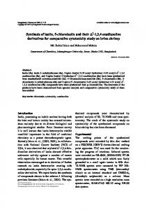
Figure 2: To a geometrical structure of the rst return map Tij . u (Ol). under the maps T0kl are strips k1l  T0kl(k0l)  ?l . accumulating on Wloc We will study, within framework of the family f , bifurcations of single round periodic orbits entirely lying in U . Such an orbit has exactly by one intersection point with +l and ?l ; l = 1; 2. Let  be some single round periodic orbit and let Pl+ and Pl? be its intersection points with +l and ?l , respectively. Then, some integers i  k1 ¨ j  k2 exist such that

P1+ 2 i01 ; P1? 2 i11 ; P2+ 2 j02 ; P2? 2 j12 :

Moreover, the following relations are ful lled

P1? = T01i (P1+ ) ; P2+ = T12(P1? ) ; P2? = T02j (P2+ ) ; P1+ = T21(P2? ) : Thus, point P1+ can be considered as a xed point of a rst return map Tij ()

de ned as the following composition of the local and global maps (Fig.2)

Tij  T21
T02j
T12
T01i : i01 ! 7 +i

(6)

Thus, the study of bifurcations of single round periodic orbits in the family f is reduced to the study of bifurcations of xed points of the rst return maps Tij () for various suciently large i and j . Formulas (3),(4) and (5) admits to nd the explicit form of the map Tij () in the initial coordinates. Below we will rescale these coordinates and parameters to the end to bring the map Tij () to some standard form.

Rescaling lemma. In some rescaled coordinates (X; Y ) the map Tij (1; 2) can be written in the following form X = Y ; (7) Y = M1 ? M2 X ? Y 2 + Ri1j2 XY + Q 1?i 2?j Y 3 + "ij where i h (8) M1 = ?d212d21  + (c21x+2 + : : :)j2 ? (y1? + : : :) 1?i 12i 22j ; M2 = ?b21c21
1 (1 + : : :)i1 1i j2 2j ;

(9)

(10) R = d
d1 [2a21d21 ? 2l02c21 ? l11b21] ; Q = d l03d 12 21 12 21 with
1 = a12d12 ? b12c12; the dots stand for terms which tend to zero as i; j ! 1 (and which are independent of (X; Y )), and "ij denote some functions such that

k"ij (X; Y; M1; M2)kC ?2 = o(j 1?i 2?j j + ji1j2j): In the rescaled coordinates (X; Y ), the domain where the map Tij is de ned includes the disc kX; Y k  Kij where Kij ! +1 as i; j ! +1. r

Proof. Choose some i and j . According to (5), for any point M (x01; y01) 2 i01, the coordinate y01 is uniquely de ned as a smooth function of x01 and y11 where y11 is the y -coordinate of the point T01i M on i11. By virtue of this, we will use (x01; y11) as the coordinates on i01. Analogously, we will use (x02; y12) as the coordinates on the strip j02, where y12 is the y -coordinate of the j -th iteration of the point by the local map T02. Then, by virtue of (5), (3) and (4), the maps T12T01i : (x01; y11) 7! (x02; y11) = and T21T02j : (x02; y12) 7! (=x01; y 11) are written as x02 ? x+2 = a12i1 x01(1 + ^1?ip1i (x01; y11)) + b12(y11 ? y1? ) +O(21i x201 + ji1x01 (y11 ? y1? )j + (y11 ? y1? )2 );

2?j y12(1 + ^2?j q2j (x02; y12)) = c12i1x01(1 + ^1?ip1i (x01; y11)) + d12(y11 ? y1? ) +O(21i x201 + ji1x01 (y11 ? y1? )j + (y11 ? y1? )2 )

and =x

j ?j 01 ? x+1 = a212 x02(1 + ^2 p2j (x02; y12)) + b21(y12 ? y2? ) + l02(y12 ? y2? )2

+O(22j x202 + jj2x02 (y12 ? y2? )j + j(y12 ? y2? )3j); =

=

1?i y 11(1 + ^1?iq1i (=x01; y 11)) =  + c21i1x02(1 + ^2?j h1j (x02; y12)) +d21 (y12 ? y2? )2 + l11i1x02(y12 ? y2? )(1 + ^2?j q2j (x02; y12)) +l03 (y12 ? y2? )3 + O(22j x202 + jj2x02(y12 ? y2? )2 j + (y12 ? y2? )4 ): Let us introduce new coordinates (;  ) de ned as

x01 ? x+1 = 1 y11 ? y1? = 1

x02 ? x+2 = 2; y12 ? y2? = 2:

(11)

The above formulas are rewritten as 2 = a12i1x+1 (1 + : : :) + a12i1(1 + : : :)1 + b12(1 + : : :)1 + 1ij (1; 1);

2?j (2 + y2? )(1 + ^2?j q2j (2 + x+2 ; 2 + y2?)) = c12i1x+1 (1 + : : :) +c12i1(1 + : : :)1 + d12(1 + : : :)1 + 2ij (1; 1); and

(12)

=  1 = a21j2x+2 (1 + : : :) + a21j2(1 + : : :)2 + b21(1 + : : :)2+

l02(1 + : : :)22 + 3ij (2; 2); = = =

1?i ( 1 + y1? )(1 + ^1?i q1i (  1 + x+1 ;  1 + y1? ) =  + c21j2x+2 (1 + : : :)+ (13)

c21j2(1 + : : :)2 + d21(1 + : : :)22 + l11j2(1 + : : :)22 + l11x+2j2(1 + : : :)2 + l03(1 + : : :)23 + 4ij (2 ; 2); where the dots stand for the constant (i.e. independent on  and  ) terms which tend to zero as i; j ! 1. Note that when deriving (12) we took into account that 21i  i1 ^1?i, 22j  j2 ^2?j . For simpli cation of formulas we have introduced the following notations. By 1ij , 2ij , 3ij and 4ij we denote the

functions of the following orders: ij i ?i 2 i 2 1 (1; 1) = O(j1 ^1 j1 + j11 1j + 1 ); ij ?i 2 (1; 1) = O(ji1 ^1 j12 + ji11 1j + 12); ij j ?j 2 j 3 3 (2 ; 2) = O(j2 ^2 j2 + j22 2j + j2 j); ij j ?j 2 j 2 4 4 (2; 2) = O(j2 ^2 j2 + j222 j + j2 j):

Besides, we will not change the notations for these functions, although the functions, in principle, will changed by transformations of coordinates. Let us substitute into the left-hand side of the second equation of (12) the expression for 1 which is given by the rst equation of (12), and into the = left-hand side of the second equation of (13) the expression for  1 from the rst equation of (13). If we dierentiate both sides of the obtained second equation of (13) with respect to 2, then the resulting equation, since d21 6= 0, = de nes 2 uniquely as a smooth function of 2 and  1 : = 2 = '(2;  1 ) = O(j 1 ^1j?i + j2jj ): It is easy to see then, that if we write, schematically, equations (12) and the rst equation of (13) in the form =

2 = 1(1; 1); 1 = 2(2; 1);  1 = 3 (2; 2) (we may do it since d12 = 6 0),then the system 2 = '(2; 1); 2 = 1 (1; 1); 1 = 2(2; 1); 1 = 3(2 ; 2); will have a unique solution (1 ; 2; 1; 2) where 1 ; 2 = O(j 1 ^1j?i + j2jj ); 2; 1 = O(j 2j?j + j1ji ): By construction, the following shift of the origin of the coordinates:

1new = 1 ? 1; 1new = 1 ? 1; 2new = 2 ? 2 ; 2new = 2 ? 2; brings the system (12) and (13) to the form

2 = a12i1 (1 + : : :)1 + b12(1 + : : :)1 + 1ij (1 ; 1);

2?j (2 + ^2?j h2(1; 1; 2)) = c12i1(1 + : : :)1 + d12(1 + : : :)1 + 2ij

(14)

and

=  1 = a21j2(1 + : : :)2 + b21(1 + : : :)2 + l02(1 + : : :)22 + 3ij

1?i(=1 + ^1?ih1(2; 2; = 1)) = [ + c21j2x+2 ? 1?i y1? + : : :]

+c21j2(1 + : : :)2 + d21(1 + : : :)22 + l11j2(1 + : : :)2 2 +l03(1 + : : :)23 + 4ij (2; 2); (15) respectively, where the functions h1;2 are uniformly bounded, as i; j ! +1, along with their derivatives, and h1 (2; 2; 0)  0; h2 (1 ; 1; 0)  0;

h1 = =1 j2O(2) + O(j=1 j + j2j) 



?




; h2 = 2 i1 O(1) + O(j2j + j1j) :

(16) Note that we have now nulli ed the constant (zero order) terms in (14) and in the rst equation of (15), and the linear ( rst order) in 2 term in the second equation of (15) is also made zero now. All zero order terms in the second equation of (15) are collected in the square brackets. It is obvious that we may de ne a new variable h i 1new = 1 + d (11+ : : :) c12i1(1 + : : :)1 + O(i1 ^1?i12 ; i11 1) 12 in such a way that the right side of the second equation of (14) would become independent of 1 , so the system will take the form (where
1 = a12d12 ? b12c12 is the Jacobian of the map T12 at the point M1? ):

2 = d
1 i1(1 + : : :)1 + b12(1 + : : :)1 + 1ij (1; 1); 12 and

2?j (2 + ^2?j h2 (1 ; 1; 2)) = d121 + O(12)

(17)

=

 1 = a21j2(1 + : : :)2 + b21(1 + : : :)2 + l02(1 + : : :)22 + 3ij (2; 1); =

=

1?i ( 1 + ^1?i h1(2; 2; 1 )) = [ + c21j2x+2 ? 1?i y1? + : : :] (18) c 12 j i 2 ? i  +c21 2(1 + : : :)2 + d b21(1 + : : :) 1 12 + d21(1 + : : :)2 12 +l11j2 (1 + : : :)22 + l03(1 + : : :)23 + 3ij (2 ; 1)24)

with some new functions h1 and h2 which satisfy (16). If we now write the second equation of (17), schematically, as

1 = '(1; 1; 2) = O( 2?j ); then it is easy to see that the equation

1 = '(0; 1; 2) de nes 1 uniquely as a function of 2: 1 = (2) = d (11+ : : :) 2?j 2 + O(j 2 ^2 j?j ): 12 Denote by S (1; 1) the right side of the rst equation of (17). By construction, if we make the coordinate transformation

2new = 2 ? S (0;  (2 )) ;

the new 2 will vanish identically at 1 = 0. Thus, after this coordinate transformation, the equations take the form 2 = d
121 i1 (1 + : : :)1 + O(ji1 ^1?i j12 + ji11 1j); (19) ? j ? j 2

2 (2 + ^2 h2 (1; 1; 2)) = d121 + O(1 ); =  1 = a21j2(1 + : : :)2 + b21(1 + : : :)2 + l02(1 + : : :)22 + 3ij (2; 2); = =

1?i ( 1 + ^1?i h1(2; 2;  1 )) = [ + c21j2x+2 ? 1?i y1? + : : :]

j (1 + : : :)

+c21 2

2 + ij 2 + d21(1 + : : :)22

(20)

+l11j2(1 + : : :)22 + l03(1 + : : :)23 + 4ij (2; 2); where ij = O(j 1?ii1j + j 2?j j2j). Like we did it before, we may shift the the coordinates 1 , 2 , 1 and 2 to some small values of order O(j 1?ii1j + j 2?j j2j), O(j 1?i21ij + j 2?j j2i1 j), O(j 1?ii1 2?j j + j 2?2j j2j) and O(j 1?ii1 j + j 2?j j2j), respectively, in such a way that the term ij 2 in the last equation of (20) would vanish, while the rest of the system (19),(20) will retain its form (without constant terms). Now, we rescale variables as follows

1 = 1u1 1 = 1v1 2 = 2u2 2 = 2 v2;

where

?i ?2j ?i ?j 1 = ? d1 d22 (1 + : : :); 2 = ? d1 d2 (1 + : : :); 21 12?j 21 12 ?j ? i i ?i
b b

1 = ? 21d 1d 2 (1 + : : :); 2 = ? 1 21d1d 21 2 (1 + : : :): 21 12 21 12 = We obtain the following system (using that h1 = O(  1 ), h2 = O(deta2 )): u2 = u1 + O( 1?i 2?j ^1?iu21 ; 1?i 2?2j u1 v1);

v2 + O(^ 2?j 1?i 2?j jv2 jjv2j + ju1j + j 2?j v1 j)) = v1 + O( 1?i 2?2j v12); l02 =u a21
1 i j 1 = d 12(1 + : : :)u2 + v2 ? d d b 1?i 2?j (1 + : : :)v22 12 12 21 21

(21)

+O(21i jj2 1?i 2?j ^2?j ju22 + j 1?i 2?j i1 j2u2 v2j + 1?2i 2?2j jv2 j3); =v = ?j ?j = 1 + O(^ 2 1?i 2 j v 1 j(jv2j + j 2j?j v 1 + ji1u2 j)) = M1 ? M2u2 ? v22

(22)

? l11d b21d
1 i1j2(1 + : : :)u2v2 + d l03d 1?i 2?j (1 + : : :)v23 21 12 21 12 where

+O(21ijj2 ^2?j ju22 + j 1?i 2?j i1 j2u2 jv22 + 1?2i 2?2j v24);

M2 = ?b21c21(a12d12 ? b12c12)(1 + : : :)i1 1?i j2 2?j i h M1 = ?  + c21j2x+2 ? 1?i y1? + : : : d212d21 12i 22j : Let us substitute the values of u2 and v2 given by (21) into (22). Then, we obtain that map Tij is written in the form l02 =u a21
1 i j 1 = d 12u1 + v1 (1 + : : :) ? d d b 1?i 2?j v12+ 12 12 21 21 o(j 1?i 2?j j + ji1j2j); =v = M (1 + : : :) ? M (1 + : : :)u ? v 2(1 + : : :) 1 1 2 1 1

? l11d b21d
1 i1j2u1v1 + d l03d 1?i 2?j v13 + o(j 1?i 2?j j + ji1j2j): 21 12 21 12

By the change of variables

U = u1 ;

V = a21d
1 i1 j2(1 + : : :)u1 + v1; 12

(23)

we nullify the linear in u1 term in the right side of the rst equation It gives

U = V (1 + : : :) ? d dl02 b 1?i 2?j V 2 + o(j 1?i 2?j j + ji1j2j); 12 21 21 V = M1 (1 + : : :) ? M2 (1 + : : :)U + a21
1 i1j2V ? V 2 (1 + : : :) (24) d12 ? l11d b21d
1 i1j2UV + d l03d 1?i 2?j V 3 + o(j 1?i 2?j j + ji1j2j): 21 12 21 12 The new linear in V term in the second equation can be immediately killed by a small shift of variables to a constant value of order O(i1j2 ). Then, after an additional rescaling of the coordinates U = Unew (1 + :::); V = Vnew (1 + :::),

system (24) is brought to the following form

U = V ? S1 1?i 2?j V 2 + o(j 1?i 2?j j + ji1j2j); V = M1 ? M2U ? V 2 ? S2 i1j2UV + S3 1?i 2?j V 3 + o(j 1?i 2?j j + ji1j2 j);

where

(25)

  S1 = d dl02 b ; S2 = l11d b21d
1 ? 2 a21d
1 ; S3 = d l03d ; 12 21 21 21 12 12 21 12

(26)

M2new = ?b21c21
1i1 1i j2 2j (1 + : : :); h i M1new = ?  + c21j2 x+2 ? 1?iy1? + : : : d212d21 12i 22j :

Next, by a coordinate transformation of the kind

X = U ? S1 1?i 2?j (V ? M1); Y = V + S1 1?i 2?j M2U + o( 1?i 2?j );

we bring system (25) to the form X = Y;

Y = M1 (1 + S1 1?i 2?j M2) ? M2 X ? Y 2 + S3Y 3

(27)

+(2S1 1?i 2?j M2 ? S2 i1j2)XY + o(j 1?i 2?j j + ji1j2j): According to (26), S i j ? 2S ?i ?j M =
1 [2a d ? 2l c ? l b ] i j (1 + : : :); 2 1 2

1 1 2

2

d12d21

21 21

02 21

11 21 1 2

hence the obtained equations coincide with (7). The lemma is proven. Remark: It follows from (25), that in the dissipative case (1 < 1 and 2 < 1) the rst return maps Tij in the rescaled coordinates is asymptotically C r?2 -close to the "parabola map" of the form

X = Y;

Y = M ? Y 2

i h where M = ?  + c21j2x+2 ? 1?i y1? + : : : d212d21 12i 22j .

3 Bifurcations of xed points in the generalized Henon map. By the rescaling lemma, bifurcations of single-round periodic orbits in the family f1 ;2 , or, that is the same, bifurcations of xed points of maps Tij with various suciently large i and j , can be studied if to know the structure of bifurcations of xed points of the generalized Henon maps of form (7). These bifurcations for map (7) with small coecients Ri1j2 6= 0 and Q 1?i 2?j were studied in [13,14] for the orientable case M2 > 0. We present here some most important results to use their next. The map (7) is asymptotically C r?2 -close to the standard Henon map3 X = Y ; Y = M1 ? M2 X ? Y 2 (28) Then, the generalized Henon map (7) will possess (as the Henon map) on the parameter plane (M1 ; M2) three bifurcational curves corresponding to bifurcations of the xed points. Namely, these curves are L+ij ; L?ij and L'ij . The map (7) has a xed point with the multiplier +1 at (M1 ; M2) 2 L+ij ; with the multiplier ?1 at (M1 ; M2) 2 L?ij ; and with the multipliers ei' ("weak focus") at (M1; M2) 2 L'ij where 0 < ' <  . The equations of the curves are as follows 2 a) L+ij : M1 = ? (1 + 4M2) (1 + :::) ; 2 b) L?ij : M1 = 3(1 +4M2 ) (1 + :::)

c)

L'ij

:

(

(29)

M1 = cos2 ? 2 cos + ::: ; M2 = 1 ? Ri1j2 cos (1 + :::)

It is necessary at least C 3 -closeness for studying bifurcations (for example, period doubling bifurcations, bifurcations of appearance of closed invariant curves etc.) Therefore, we consider C -smooth dieomorphisms with r  5. 3

r

Figure 3: Elements of the bifurcation diagram for generalized Henon map on the half-plane M2 > 0 in the case Ri1j2  0. where the ellipsis denote terms tending to zero as i; j ! 1. Note that the curve L'ij has been written in the parameter form (where the angle argument , 0 < <  , of multipliers of the "weak focus" is the parameter). The bifurcations curves on the half-plane M2 > 0 are shown in the Fig.3 for the case where Ri1j2 < 0. Also we shown here some elements of reconstructions of phase portraits at transition across the bifurcation curves. Note that the following formula [13] i j R G1 = 16(1 ?1cos2 ) (1 + :::)

(30)

takes place for the rst Lyapunov value of the "weak focus" at (M1 ; M2) 2 L'ij . It means that in the case Ri1j2 < 0 a stable invariant closed curve is born at transition (from left to right) across the curve L'ij (see Fig.3). In the case Ri1j2 > 0 an unstable invariant closed curve is born at the transition from right to left across the curve L'ij .

Figure 4: Elements of the bifurcation diagram near the point B ?? . We can nd on the parameter half-plane M2 > 0 four points which are (at least) codimension two bifurcation points, Bij++ , Bij?? , Bij2=3 and Bij=2 , such that the map has a xed point with multipliers 1 = 2 = +1, 1 = 2 = ?1, 1;2 = ei2=3 and 1;2 = ei=2 , respectively. It was established in [13,14] that the rst three points are nondegenerate if R 6= 0 and the point Bij=2 is nongenerate if R 6= 0 and R ? 2Q
(b21c21
1 )?1 6= 0. The point Bij?? will be of a special interest for us. In the case Ri1j2 < 0 the bifurcation diagram for the restricted ow normal form (so-called "HorozovTakens normal form") in a small neighbourhood of the point Bij?? will be such as in gure 4 [15,16]. Here stable and unstable limit cycles will coexist at values of parameters M1 and M2 from the regions (4) and (5) (the shaded regions in gure 4) adjoining to the point Bij?? . In the case Ri1j2 > 0 analogous regions of the parameters exist where the Horozov-Takens normal formich possesses stable and unstable limit cycles, see, for example, [17]. It can be shown that there exist subregions in (4) and (5) adjoining to the point Bij?? and such that the map (7) has, at corresponding values of the parameters, stable and unstable closed invariant curves. We will denote these regions as Dijsuc .

Thus, in the case of the generalized Henon map with R 6= 0 we can always detect on the half-plane M2 > 0 of the parameters (M1; M2) three domains Dijs , Diju and Dijsuc such that the map has a stable xed point at (M1 ; M2) 2 Dijs , a completely unstable xed point at (M1; M2) 2 Diju and stable and unstable closed invariant curves at (M1; M2) 2 Dijsuc .

4 On the structure of bifurcation sets for singleround periodic orbits of the family f  . 1 2

Now we are able to recover a bifurcation picture for single-round periodic orbits in the case of the family f1 2 . We can use formulas (8) and (9) to nd relations between the initial and rescaled parameters, i.e. between (1 ; 2) and (M1 ; M2). By such a way we can construct bifurcation curves L+ij ; L?ij and L'ij on the plane (1 ; 2). Note, that a xed point of the rescaled map Tij corresponds to a single-round periodic (of period (i + j + n1 + n2 )) orbit of f1 ;2 and a closed invariant curve of the rescaled map corresponds to a periodic closed invariant curve of f1 ;2 : let Cij be such a curve and Cij0 be its connected components on i01, then, fi+1 ;j +2 n1 +n2 (Cij0 ) = Tij (Cij0 ) = Cij0 .

Proposition 1 Let f1;2 be the two-parameter family under consideration and f0 be the orientable dieomorphism. Let S be a small neighbourhood of the origin on the parameter plane (1 ; 2). Then, a countable set of curves L+ij ; L?ij and L'ij exists in S for any  > 0. Curves L+ij and L?ij accumulate on the segment I  S of the axis 1 = 0. Moreover, for any point 2 2 I there are in nite sequences fin(2 )g and fjn (2 )g of integers such that curves L'i j accumulate at 2 as in ! 1 and jn ! 1. n n

Proof. Consider the equation (29a) for the curve L+ij and rewrite it in the initial parameters (1 ; 2). Parameters M1 and 1 are connected by formula (8). In order to establish a relation between M2 and 2 consider equation (9). In the orientable case this equation can be written in the form

(31) M2 = A1i 2j ; where A = jb21c21
1(1 + : : :)j, l = jl l j; l = 1; 2. Thus, M2 > 0 in this case.

Take the logarithm from both sides of (31). One has 1 ln M2 = i + j ln 2 () : ln 1 A ln 1 () Since   ln  (0) ln  (  ) 2 2 2 = ? ln  () ? ? ln  (0) =  () ? 0 ; 1

1

(32)

by virtue of (1), we can rewrite (32) as follows 2 = ji ? 0 ? j ln1 ln MA2 : 1 Thus, we can rewrite (33) in the form

(33)

(34) M2 = A1i?j(0 +2 ) ; and, by virtue of (29), the equation of curve L+ij takes the following form

i?j (0 +2 2 1 = 1?i y1? ? c21j2x+2 + rij + (1 + A1 4d2 d ) (1 + :::) 1?2i 2?2j ; (35)

12 21

where rij = o(jj2j + j 1?ij). Analogously, the equation of curve L?ij can be written in the form i?j (0 +2 ) 2 1 = 1?iy1? ? c21j2 x+2 + rij ? 3(1 + A1 4d2 d ) (1 + :::) 1?2i 2?2j ; 12 21 (36) + ? It is easily to see from these formulas that curves Lij and Lij accumulate on the segment j2 j   of the axis 1 as i ! 1 and j ! 1. Concerning curves L'ij , these curves absent in S for some i and j . Indeed, formulas (34) and (29) show that the following relation has to be ful lled for parameter 2 on any curve L'ij or

1 ? Ri1j2 = A1i?j (0 +2 ) ;

2 = ji ? 0 + j lnlnA + O(i1j2)

(37)

1

Since j2 j <  , the equality (37) can be ful lled only for such i and j that

j ji ? 0j < 

This inequality has in nitely many integer solutions in i and j for any  > 0. It implies that a countable set of curves L'ij exists in S . Moreover, formula (37) shows that every point (0; 2) 2 S is a limit point for some set of curves L'ij . Indeed, let in and jn be in nite integer-valued sequences such that the fractions in =jn converge to (2 + 0 ). It follows from (37) that curves L'i j accumulate at the point (0; 2) as n ! 1. This completes the proof of proposition 1. Formulas (8) and (9) allow us to construct on the parameter plane (1 ; 2) bifurcation curves L+ij ; L?ij and L'ij and as well as to detect the domains Dijs , Diju and Dijsuc for various i and j . As a direct consequence of proposition 1 we obtain that in nitely many domains Dijsuc lie in S , and, in particular, the following proposition holds n n

Proposition 2 On the parameter plane (1; 2) in any neighbourhood of ori-

gin there exists a countable set of domains Dijsuc , accumulating at (0; 0) as i ! 1 and j ! 1, such that the dieomorphism f1 ;2 has at (1 ; 2) 2 Dijsuc the stable and unstable closed invariant periodic curves.

Propositions 1 and 2 are valid in the case where f0 has a non-orientable heteroclinic cycle, but the proofs are slightly dierent. Namely, we act here as follows. If one of the saddle points O1 or O2 is non-orientable, i.e., it has one negative multiplier, then we take the integers i and j of an appropriate parity. If one of the global maps, T12 or T21, has negative Jacobian, we nd, using [10], in the Newhouse region
i a dense subset of parameters corresponding to the existence of a orientable nontransversal heteroclinic cycle (for example, with orientable two-round global maps T^12 = T12T01n T21T02m T12 or T^21 = T21T02q T12T01p T21 for suciently large integers n; m; p and q). Evidently, propositions 1 and 2 are valid for such the heteroclinic cycles.

5 The proof of main theorems. We give the proofs of theorems A and B in the following order: rst we prove theorem B and, next, we show that theorem A follows from theorem B. The proof of theorem B. First of all, we note that regions
i from theorem B are Newhouse regions of the rst type (with heteroclinic tangencies) on the parameter plane (1 ; 2). The existence of such regions can be deduced from the proof of main theorem from [10] (see theorem 4 there) by a simple repetition of arguments for the case of two-parameter families. The main characteristic property of regions
i is as follows. Values of (1 ; 2) are dense in
i such that dieomorphism f1 ;2 of the family has a simplest nontransversal heteroclinic cycle containing the points O1 () and O2 () and the family unfolds generally this heteroclinic tangency.

After this, theorem B is deduced easily from our results by means of the embedded disks method. Indeed, let 1 2
i . Arbitrary closely to 1 there exists a value  = 1 2
i such that dieomorphism f1 has a simplest nontransversal heteroclinic cycle containing points O1(1 ) and O2 (1). This cycle is of mixed type. By proposition 2, in any neighbourhood of 1 in
i there is an open neighbourhood 1 such that dieomorphism f at  2 1 has stable and unstable invariant closed curves (1 corresponds to some region suc ). Further, we nd inside 1 such  =  that f has a from regions Djk 2 2 simplest mixed type nontransversal heteroclinic cycle. Again by proposition 2, a neighbourhood 2  1 exists such that dieomorphism f at  2 2 has two stable and two unstable invariant closed curves, etc. Thus, we obtain a

countable sequence of embedded discs

1  2  :::n  :::

(38)

such that at  2 n dieomorphism f has n stable and n completely unstable invariant closed curves. It completes the proof of theorem B. Remark. In nite sequence (38) can be supplemented by embedded disks corresponding to the existence of stable, completely unstable and saddle periodic orbits. Thus, we obtain that in regions
i values of parameters  are dense corresponding to dieomorphisms with in nitely many stable, completely unstable and saddle periodic orbits as well as stable and completely unstable invariant closed curves. The proof of theorem A. Let a dieomorphism g have hyperbolic saddle periodic orbits P1 ; :::; Pn and let ?~ ii+1  W u (Pi ) \ W s (Pi+1 ) ; ?~ n1  W u (Pn) \ W s(P1 ) ; i = 1; :::; n ? 1 . We can suppose, without of loss of genericity, that all pointed out intersections are transverse and only one of them, let us say the intersection of the manifolds W u (Pn ) and W s (P1 ) , is nontransversal. Moreover, we cam suppose that W u (Pn ) and W s (P1) have a quadratic tangency in the points of the heteroclinic orbit ?~ n1 . Let this cycle be of neutral type. Then, we will nd near g a dieomorphism with a simplest neutral non-transversal heteroclinic cycle. Let q be such an integer that the points of periodic orbits P1 ; :::; Pn are xed points for the map g q . We choose up to one point, Oi ; i = 1; :::; n , from every orbit Pi and consider for the map g a heteroclinic cycle consisting of the xed points O1 ; :::; On and heteroclinic orbits ?ii+1  ?~ ii+1 , ?n1  ?~ n1 , where orbits ?ii+1 of dieomorphism g consist of taken in q iterations corresponding points of orbits ?~ ii+1 of g . Thus, the dieomorphism g q has the heteroclinic cycle such that the intersection of manifolds W u (Oi ) and W s (Oi + 1) ; i = 1; :::; n ? 1; along the orbit ?ii+1 is transverse and W u (On ) has a quadratic tangency with W s (O1) in the points of the orbit ?n1 . By hypothesis of the theorem, saddle values of at least two points from the set fO1; :::; Ong lie in dierent sides from one. First, we consider the case where these points are O1 and On . Since the intersections of W u (Oi ) and W s (Oi + 1) ; i = 1; :::; n ? 1; are transverse, it follows, by virtue of the C r --lemma that there is a heteroclinic orbit ?1n , ?1n  U , along which manifolds W u (O1) and W s (On ) intersect transversally. Let us consider the heteroclinic cycle C = fO1; On; ?1n ; ?n1 g . Evidently, it is the simplest structurally unstable heteroclinic cycle. Consider now the case where saddle quantities of the points O1 and Oj , j 2 f2; :::; n ? 1g , are in the dierent sides from one. Let us take some heteroclinic orbit ?1j  U along which manifolds W u (O1) and W s (Oj ) intersect transversally . Consider a non-transversal heteroclinic point M1+ 2

s (O1) \ W u (On ) and its a neighbourhood + . Denote by lu a connected Wloc 0 1 piece of the set W u (On) \ +1 which contains the point M1+ . It follows again from the C r --lemma that an in nite number of curves wk from the set W u (Oj ) \ +1 lies in +1 and these curves accumulate on l0u as k ! 1 .

Thus, we can split the initial heteroclinic tangency in such a way that some s (O1) \ + . curve wk (with large k) will have a quadratic tangency with Wloc 1 Respectively, the new dieomorphism g~q has a nontransversal heteroclinic orbit ?jk at whose points the manifolds W u (Oj ) and W s (O1) have a quadratic tangency. Thus, the cycle C~ = fO1; Oj ; ?1j ; ?jn g is the simplest neutral nontransversal heteroclinic cycle. Theorem B can be applied to this cycle, that completes the proof. The authors thank D.V.Turaev for helpful discussions. This work was supported in part by the grant of INTAS No. 2000-221 and by the grant of RFBR No. 99-01-00231.

References [1] S.E.Newhouse, Publ. Math. IHES., 1979, v.50, 101{151. [2] S.V.Gonchenko, D.V.Turaev, and L.P.Shilnikov, Russian Acad. Sci.Dokl.Math., 1993, 47(2), 268-273. [3] J.Palis, M.Viana, Ann.Math., 1994, v.140, 207{250. [4] N.Romero, Ergod.Th. & Dynam.Sys., 1995, v.15, 735{757. [5] S.V.Gonchenko, D.V.Turaev, and L.P.Shilnikov, Russian Acad. Sci. Dokl. Math., 1993, 47(3), 410-415. [6] S.V.Gonchenko, D.V.Turaev, and L.P.Shilnikov, Soviet Math.Dokl., 1992, 44(2), 422-426. [7] S.V.Gonchenko, D.V.Turaev, and L.P.Shilnikov, Physica D, 62(1-4), 1-14. [8] S.V.Gonchenko, D.V.Turaev, and L.P.Shilnikov, Chaos, 1996, 6(1), 15-31. [9] S.V.Gonchenko, D.V.Turaev, and L.P.Shilnikov, Proc. of Int.Conf. dedicated to 90-th of L.S.Pontryagin, VINITI, 1999, 67-129. [10] S.V.Gonchenko, D.V.Turaev, and L.P.Shilnikov, Proc. of the Steklov Inst. of Math., 1997, v.216, 7-118. [11] S.V.Gonchenko, L.P.Shilnikov, Ukr. Math.J., 1990, 42(2), 134-140. [12] S.V.Gonchenko and L.P.Shilnikov, Russian Acad. Sci. Izv. Math., 1993, 41(3), 417-445. [13] S.V.Gonchenko and V.S.Gonchenko, Preprint No.556, WIAS,Berlin, 2000. [14] S.V.Gonchenko and V.S.Gonchenko, to be published (Proc. of Math.Steklov Inst., Moscow). [15] F.Takens, Comm.Math.Inst., Rijkuniversitet Utrecht, 1974, 2, 1-111. [16] E.Horozov, Proc.Petrovskii Seminar, Moscow Univ., 1979, 5, 163-192. [17] Yu.A.Kuznetsov, Elements of Applied Bifurcation Theory, Applied Mathematical Sciences, v.112, 1995, Springer-Verlag.