workweek length of labor, maybe another important cause of drop in output if you consider a nation of workaholics like Japan. In this paper, I have tried to bring ...
Accounting for the ‘Lost Decade’ in Japan
Suparna Chakraborty Department of Economics, University of Minnesota 1035 Heller Hall, Minneapolis, MN 55455 and Research Department, Federal Reserve Bank of Minneapolis 90 Hennepin Avenue, Minneapolis, MN 55401
____________________________________ I thank V V Chari for his continuous support and advice. I also thank Michele Boldrin and Fumio Hayashi for their help with my research. I have also benefited greatly from conversations with the participants of the Economic Growth and Development workshop at University of Minnesota and the participants at the 2004 Midwest MacroEconomics Meetings held at Iowa State University, Ames, Iowa. The remaining errors are mine. The views expressed herein are those of the author and not necessarily those of the Federal Reserve Bank of Minneapolis or the Federal Reserve System.
Abstract There is no debate amongst economists that Japan performed poorly during the1990s. This can be seen in falling growth rates of GDP per capita, investment per capita and mounting problems of non performing loans and ballooning Government deficit. A lot of models have tried to come up with an explanation for the Lost Decade. However, none of them have yet been able to clearly account for the growth slump. At this point, it is necessary to revisit all possible distortions that might have caused the dismal performance during the 1990s. This would help us to correctly identify the possible problem areas and search for more specific causes of downturn of the economy in a considerably narrowed field. In this paper, I have tried to bring together the different proposed theories in a consolidated way to help isolate promising theories from not so promising ones. To do so, I applied the Business Cycle Accounting procedure developed by V V Chari, Ellen R McGrattan and Patrick Kehoe to the Japanese case. I find that efficiency wedge is important in explaining the dismal performance of the Japanese economy during the 1990s but labor wedge is not very important except for a brief span of time during 1996 to 1997. My most important result is that investment wedge played a major role in the performance of the Japanese economy during the 1990s. So, any model that tries to focus on what went wrong in Japan in 1990s would do well to focus on frictions on productivity and investment financing that might be at the root of the dismal performance of the Japanese economy.
2
Introduction
Japanese economy has performed very well from after the 2nd World War to about the 1980s. The average growth rate of the GDP per capita was a stellar 8.09% from 1955 to 1973; it stabilized to about 3.02% from 1973 to 1991, which was much more than the average growth rate of GDP per capita of 2% in United States. However, in the 1990s the performance of the Japanese economy was dismal. The average growth rate of GDP/capita fell to .72%, an all-time low since 1955. If we look at the average growth rates of investment during the above periods, investment per capita grew at an average rate of 14.06% during 1955 to 1973, then it stabilized at 2.19% from 1973 to 1991; but the average growth rate of investment fell to -.04% during 1991 to 2001. Japan’s enviable growth rate till about the late 1980s has attracted much attention. As explained by Professor Anne O Krueger in her article “East Asian Experience and Endogenous Growth Theory”1, Japan’s productive capacity was seriously impaired after the 2ndWorldWar. Japanese Government used a policy of quantitative restriction on imports and promotion of exports to promote production. This policy was gradually liberalized over the years. However, as analyzed by Lawrence in 1991, restrictions may have taken the form of industrial organizations like the Keiretsu. Also, during the 1980s there is evidence to suggest preferential credit rationing, with substantial credit going to exporters. The labor market institutions with strong job
1
East Asian Experience and Endogenous Growth Theory published in “Growth Theories in
Light of the East Asian Experience” edited by Takahasi Ito and Anne O Krueger
3
protection, intensive on-the-job training and enterprise helped Japan to utilize imported technology rapidly and successfully. All these policies led to the phenomenal growth rate of Japan’s GDP per capita during the recovery period after the 2nd World War till about 1980s.The question is what caused the dismal performance of Japanese economy in the 1990s after about 50 years of exemplary growth? Many theories have been forwarded to explain the Japanese slump during the 1990s. The slump has been blamed on inadequate fiscal policy, the over-investment in the earlier years resulting in depressed investment later on; and problems of financial intermediation. In a recent article2, Edward Prescott and Fumio Hayashi proposed an alternative explanation. They have claimed that the reasons for the downturn in 1990s was not any problems of investment financing, but rather slump in total factor productivity and fall in workweek hours.
In this paper, I shall attempt to explain which factors might have been important in explaining the downturn of Japanese economy in 1990s. I shall use the Business Cycle Accounting approach3 developed by V V Chari, Ellen Mcgrattan and Patrick Kehoe to try to account for the drop in downturn by a drop in productivity factor, drop in work-week hours or any investment frictions.
2
3
‘The 1990s in Japan: A Lost Decade’ –Review of Economic Dynamics, 2002 Volume 5 “Business Cycle Accounting” NBER Working Paper No. w 10351, March 2004
4
The plan of the paper is as follows.
In Section 1, I shall first provide some facts about the Japanese economy before and during the downturn in 1990s.
Section 2 is an exposition on the Business cycle accounting methodology. I provide a summary of theoretical equivalence results proposed by V V Chari, Ellen Mcgrattan and Patrick Kehoe.
In Section 3, I provide a model for Business Cycle Accounting used by me in this paper.
In section 4, I provide the results generated by applying the Business Cycle Accounting procedure to the Japanese case.
5
Section 1
Facts about the Japanese Economy during the ‘Lost Decade’
1.1 Poor Performance in the 1990s
We begin with an examination of the Japanese National Income Accounts data for 1955 to 2001. As already stated in the introduction, Japanese economy has performed very well from after the 2nd World War to about the 1980s. This was evident in the average growth rate of GDP per capita which stood at 8.09% from 1955 to 1973; it then fell to about 3.02% from 1973 to 1991. This growth rate was still much more than the average growth rate of GDP per capita of 2% in United States. However, in the 1990s the performance of the Japanese economy was dismal. The average growth rate of GDP/capita fell to .72%, an all-time low since 1955. Another indicator of this dismal performance is the average growth rates of investment during the above period.
Investment per capita grew at an average rate of 14.06% during 1955 to 1973, then it stabilized at 2.19% from 1973 to 1991; but the average growth rate of investment fell to -.04% during 1991 to 2001. In this scenario, Government tried to keep the pace of the domestic economy by a steady expenditure over the periods. Government expenditure stood at an average of 3.3% during 1955 to 1973; the average rate of growth of per capita government spending then fell to 2.6% from 1973 to 1991. During 1991 to 2001, the average rate of growth of per capita government spending was 1.6%. Refer to Figure 1 for a graphical exposition of these trends.
Looking at the above figures, it seems like the Japanese economy was doing very well up to the 1980s poised to catch up with the United States, but something went wrong in the 1990s. After
6
maintaining decades of high growth rates, the GDP per adult in 2001 fell to 83.9% of what it should have been if the average growth rate of 3.02% during the 1980s could have been maintained in 1990s.
1.2 Workweek falls in 1988-1993 period
Japan’s strong labor market was credited for its role in the remarkable recovery and high growth rate of Japanese economy after the Second World War Aside from the fact that in-the-job training and job protection resulted in a skilled labor force, the hours worked per week averaged at 44 hours during 1980 to 1992. However, during 1988 to 1993 due to huge support amongst the Japanese population, the Labor Standards Law was modified. The new legislation reduced workweek from 6 to 5 days a week, it added one day to paid vacation and increased the number of national holidays by three. The result of this change in legislation was a fall in average hours worked to 40 hours per week during the 1990s. This is what Figure 2 depicts. However, during the period of 1980 to 2001, we notice a slight increase in the employment to working population (people aged 15-64) ratio from .7 in 1980 to .74 in 2001. This trend is illustrated in Figure 3. Hence even though the modified Labor Standards Law did have an effect on the workweek hours, the negative impact on overall man hours worked was to some extent reduced due to slight increase in employment.
1.3 Investment per working population in 1990s
The investment to GDP ratio in Japan has always been higher than in United States. The average investment to GDP ratio during 1955 to 1973 stood at .17 in US as opposed to.23 in Japan. During 1973 to 1991, the investment to GDP ratio was .17 in US but increased to .29 in Japan. It
7
remained at .19 in US and .3 in Japan during 1992-2001. So, investment has always been a big part of GDP in Japan. But, during the slump of 1990s, investment per working population fell by an average of .04%. This has caused some concern and has generated many theories. A majority of these theories credit a fall in bank loans as causing the fall in credit availability, which caused a fall in investment. Taking a closer look at investment finance done by firms from the period 1984 to 2000, Prescott and Hayashi are of the view that supply of loans did not decline, as there were other sources of finance apart from bank loans that acted as a buffer against the drop in bank loans. Alongside this observation, if there was also enough demand for loans for investment, then we should see investment growing. However, data on investment during this period seems to suggest the contrary.
Aggregate investment comprises of three components: investment in Plant & Machinery by private sector, investment in dwellings by private sector and investment by public sector. During the 1980s in Japan land prices were soaring before it crashed during the 1990s. So, we might expect people to anticipate crashing value of investment value of land in future, and thus decrease investment in land and dwellings.
However, if there are ample investment opportunities and no credit crunch, we should see enough investment in plant and machinery by private sector. This necessitates a look at breakdown of investment to look at what happened?
Aggregate Investment = Gross Fixed Capital Formation (Plant & Equipment+Dwellings+Public investment) +Change in inventories.
8
The average growth rate of investment in dwellings per working population stood at 1.92% (1980:1991) and it fell to -2.1% (1992:2001). The average growth rate of investment in plant & equipment per working population stood at 7.05% (1980:1991) and it fell to -.07% (1992:2001). This was compensated by the average growth rate of public investment per working population. The growth rate was .29% (1980:1991) but it increased to 1.88% (1992:2001). Figure 4 depicts the share of investment to GDP by type of investment.
There seems to be 3 distinct trends in investment. Investment in Plant & Equipment to GDP ratio increased from 1980 to 1991, then slumped during 1992 to 2001 except for a brief period of increase from 1996 to 1998.
Investment in dwelling to GDP ratio and Investment in public sector to GDP ratio follow a similar trend. They both fell from 1980 to 1985 and grew from 1986 to 1990 and again fell from 1996 to 2001; except for 1991 to 1996 when Investment in dwelling to GDP ratio falls and Investment in public sector to GDP ratio rises, which suggests that when the slump hit the economy around 1991-1992, and there was a fall in investment, government increased public investment. This suggests that even if supply of funds for investment was not constrained, but investment did not take place at the same rate as it had during 1980 to 1991. This opens up the possibility that even though supply of funds was not constrained to firms but demand of funds for investment by private sector was constrained. In a later paper, we explore the option that if firms offer land as collateral to banks to borrow funds for investment, then crashing land prices would decrease the value of collateral and thus constrict funds that are available for investment. This might explain the fact that even if there are enough investible funds in supply, but collateral constraints prevent these funds from being channeled to promising investment projects.
9
Section 2
Business Cycle Accounting
In the paper .Business Cycle Accounting., VV Chari, Ellen R Mcgrattan and Patrick Kehoe show that large classes of business cycle models are equivalent to a prototype growth model with time-varying wedges that, at least at face value, look like time-varying labor taxes, investment taxes and productivity.
The authors refer to these wedges as labor wedges, investment wedges and efficiency wedges. Different theories have been forwarded to explain a fall in output during depression: it can be caused by a fall in productivity, which can be due to a negative shock to technology or input financing frictions that result in movement of inputs to inefficient firms rather than efficient firms. Output can also fall if there are increased wedges due to unionization or any other labor market frictions that make labor costly. Investment frictions affect output by making investment more expensive. In a theoretical exposition, the authors show how a model with input financing frictions can be mapped into a model with efficiency wedge. The authors also show similar equivalence results between models with labor-unions and a growth model with labor taxes; and a model of investment frictions (Carlstrom & Fuerst 1997) with a growth model which incorporates investment taxes. These equivalence results propose a method of accounting for economic fluctuations using a business cycle model with
10
appropriate taxes incorporated in it. The method is to use a parameterized growth model to measure the wedges from the data. The wedges are then fed back into the growth model individually and in various combinations to assess what fractions of the output movement can be attributed to each wedge separately and in different combinations. The goal is to identify what kind of frictions should be considered to deliver the quantitatively relevant types of wedges that are observed in the prototype growth economy.
2.1 The Model
I am using a prototype growth model with time varying efficiency, labor taxes and investment taxes to account for the output slowdown of Japan during the 1990s. I shall refer to the time varying efficiency as an efficiency wedge; the time varying labor tax as a labor wedge and the time varying investment tax as an investment wedge. My aim is to identify wedges that can significantly explain the drop in GDP per working population in Japan during the 1990s. For details, please refer to “Business Cycle Accounting”, VV Chari, Ellen Mcgrattan and Patrick Kehoe.
This procedure would thus suggest types of models that would be promising in explaining the lost decade of Japanese economy in 1990s. For example, if we find that investment wedge is relevant in explaining the drop of output per working population then we have to look for models that can provide a channel or investment friction, the likes of Carlstrom & Fuerst -1997, or Bernanke & Gertler - 1989. The prototype economy is a growth model with three stochastic variables: the efficiency wedge At ; the labor wedge τ nt ; the investment wedge τ xt .
11
The economy every period consists of N t identical agents. The representative agent chooses per capita consumption ct ; per capita investment xt ; per capita labor lt ; to maximize present discounted value of lifetime utility.
Thus the representative consumer’s problem can be stated as: ∞
Max
ct , xt ,lt
E0 ∑ N t β t u (ct ,1 − l t ) t =0
subject to : 1. N t (ct + xt (1 + τ xt )) ≤ N t ( wt l t (1 − τ nt ) + rt k t + Trt ) ∀t 2. N t +1kt +1 ≤ N t ( xt + (1 − δ )kt ) ∀t 3. ct ≥ 0; kt +1 ≥ 0; 0 ≤ lt ≤ 1 ∀t where subscript t denotes the time period t, kt is the beginning of the period capital stock, τ nt is the tax rate on labor income, which we shall refer to as labor wedge, τ xt is the tax rate on investment, which we shall refer to as the investment wedge, wt is the wage rate, rt is the rental rate on capital, Trt is the per capita transfer from the government. We shall assume that population grows at a constant rate of g n ; and technology grows at a constant rate of g z and the depreciation rate of capital stock is δ .
There is a representative firm in the economy, which produces the final good using labor and capital. The firm chooses per capita labor lt and per capita capital kt to maximize profits every period given production technology of the final output, yt .
12
Thus the representative firm’s problem can be stated as:
Max
k d t ,l d t
yt − wt l d t − rt k d t
subject to : 1. yt ≤ At F (kt , (1 + g z )t lt ) ∀t 2. yt ≥ 0; ∀t
where At is the time-varying productivity that we shall henceforth call efficiency wedge. Notice that if the economy were on a balanced growth path, then At should be constant over time. Shocks to At would cause output to deviate from its value on a balanced growth path.
I assume that government balances its budget every period, so that N t ( g t + Trt ) ≤ N t (τ nt wt lt + τ xt rt xt ) ∀t
where gt is the per capita government expenditure. I shall further assume that government expenditure on goods is wasted every period and does not enter representative agent’s utility function.
Every period the resource constraint is satisfied: 1.N t yt ≥ N t (ct + xt + gt ) ∀t 2. ltd ≤ lt ∀t 3. ktd ≤ kt ∀t
13
Notice that if there are no wedges, i.e. we set the time varying efficiency wedge to a constant value and assume no taxes on labor income or investment expenditure, i.e. τ nt =constant; τ xt =constant ∀t ; then the economy would be on a balanced growth path. However, if there are shocks to either the productivity wedge, or any labor market friction or investment financing friction, then it would distort the margin such that marginal rate of substitution between leisure and consumption will diverge from the marginal productivity of labor; and the intertemporal marginal rate of substitution of consumption would diverge from the marginal productivity of capital; also the output would diverge from the balanced growth path output; thus the time-varying efficiency factor At along with the taxes on labor income τ nt and investment the economy to move away from the balanced growth path.
14
2.2 How the model works, the technical and algebraic details:
Denote any variable zˆt =
zt (1 + g z )t
i.e. a variable zt discounted by the long term growth rate of technological development. Solving the above problem we get the following equations:
At =
yˆt F (kt , (1 + g z )t lt )
un (ct , (1 − lt )) = (1 − τ nt ) At Fl (kt , (1 + g z )t lt ) uc (ct , (1 − lt ))
(1) (2)
β Et uc (ct +1 , (1 − lt +1 )){ At +1 Fl (kt +1 , (1 + g z )t +1 lt +1 ) + (1 + τ xt +1 )(1 − δ )} = (1 + g z )t (1 + τ xt )uc (ct , (1 − lt )) (3) cˆt + (1 + g n )(1 + g z )kˆt +1 − (1 − δ )kˆt + gˆ t ≤ yˆt (4)
Now given the state of the economy described by the wedges, st = ( At , τ nt , τ xt , gˆ t ) and the capital stock, kˆt we can get solutions to the decision variables:
yˆt = yˆt ( st , kˆt ) cˆ = cˆ ( s , kˆ ) t
t
t
(5) (6)
t
lt = lt ( st , kˆt ) kˆ = kˆ ( s , kˆ ) t +1
15
t +1
t
t
(7) (8)
Section 3
Measuring the wedges
3.1 Data availability
In my accounting procedure, I use data to estimate the stochastic process for the wedges and then measure the realized wedges once the parameters of the stochastic process are known. I shall concentrate on the period from 1980 to 2001. My assumption is that in 1980 economy is poised to be on a balanced growth path. If we look at the growth rate of GDP per working population, it had stabilized to about 3.02% during 1973 to 1991.This seems to suggest that Japanese economy was poised on a balanced growth path during 1973 to 1991. Throughout I am using annual data for Japanese variables in 1995 constant prices in US dollars. I have the data on GDP, Gross Fixed Capital Formation (private enterprises and public), Net change in inventories (private enterprises and public) Private Consumption Expenditure, Government Consumption Expenditure and Net Exports. I construct Gross Capital Formation as the sum of Gross Fixed Capital Formation (private enterprises and public) and Net change in inventories (private enterprises and public). An accounting convention that I follow throughout this paper is to include the Government investment in total Investment of the economy; and to include net exports to private consumption to give me a measure of domestic consumption. We also have data on population by age, employment
16
and monthly hours of work. The data is available from SourceOECD or Japan Statistical Yearbook; and the Japan Population Census. The ILO-LABORSTA gives the data on monthly hours worked (these data are adjusted for discrepancies in estimates of Labor Force Survey and Establishment Survey).
Our working population, N t =Population aged 15 to 64.
I can therefore calculate the per capita GDP ( yt ), Gross Capital Formation ( xt ), Consumption ( ct ), Government ( gt ) and Net Exports.
The accounting convention I follow is:
Ct = Private consumption +Net Exports
X t = Gross capital formation (private and public enterprises)
Gt = Government Consumption Expenditure. Hence, GDP Yt = Ct + X t + Gt
Per capita variable zt =
Zt . We can construct the capital stock series, given X t ; Nt
and the initial capital stock k0 by the Perpetual Inventory Method, kt +1 = xt + (1 − δ )kt
17
3.2 Estimating the Stochastic Process for the Wedges
The first step in my analysis is to estimate the efficiency, labor and investment wedge every period from the model equations and the data. So, given the data on consumption, labor, capital stock and an estimate of the parameters of the model, we can use equations (1)-(4) to estimate the wedges. Equation (1) would give me the efficiency wedge series At and Equation (2) would give me the labor wedge series τ nt . It should be noted that investment wedge cannot directly be calculated from the given equations because we need to specify expectations over future values of consumption, the capital stock, and wedges and so on. The decision rules from my model implicitly depend on these expectations and therefore on the stochastic process driving the wedges. Thus, the estimated stochastic process is important only for measuring the investment wedge.
We estimate the stochastic process for wedges as follows. We shall assume that production function has the form At F ( kt ,1 − lt ) = At ktθ ((1 + g z )t lt )1−θ ; the utility function has the form u (c,1 − l ) = log c + ψ log(1 − l ) . We choose θ = .36; β = .972; δ = .089 and ψ = 1:13 (the parameters are from Edward Prescott and Fumio Hayashi). The time endowment is taken as 5000 hours annually.
18
Using the production function and the utility function specified before, we can reduce equations (1)-(4) to:
At =
ψ 1−θ
β Et
*
yˆt θ 1−θ ˆ kt lt
(9)
cˆt l * t = (1 − τ nt ) (10) yˆt 1 − lt
1 θ kˆt +1 1 + (1 + τ xt +1 )(1 − δ )} = (1 + g z ) *(1 + τ xt ) * (11) { cˆt +1 yˆt +1 cˆt cˆt + (1 + g n )(1 + g z )kˆt +1 − (1 − δ )kˆt + gˆ t ≤ yˆt (12)
We first need to figure out the stochastic process for the wedges. We know the data on yt , ct , lt and g t . So, the government wedge gt is taken from the data. We can figure out the efficiency wedge At and labor wedge τ nt from equations 9 and 10. So, if we can figure out investment wedge τ xt we can figure out the stochastic process for wedges. To do this, we first need a procedure to solve my non-linear model. I shall use the Method of Log Linearization suggested by King, Plosser and Rebelo (1988)4. The method involves writing the model equations that solve the decision variables, solve for the steady state of the model and log linearizing
4
Robert King, Charles Plosser, Sergio Rebelo (1988), “Production, growth, and
business cycles: The basic neoclassical model”, Journal of Monetary Economics 21(2), pp. 195-232.
19
the model equations around the steady state. Finally, I shall use the Method of Undetermined Coefficients to solve for the decision rules. Notice that given my functional form specifications and my model, in the absence of distortionary wedges, the economy would be on a balanced growth path with output per capita, consumption per capita, investment per capita all growing at the rate of technological progress, g z and labor would be constant over time. So, to solve for a steady state for the model, I need to discount all variables on the balanced growth path by their growth rate on the balanced growth path, g z . This is what is depicted in equations (9) to (12). Then we can get the steady state values of the variables by solving equations (13) to (16). The first step is to find the steady state values of the wedges. I shall choose the initial condition for the wedges such that in the starting year, one that I choose to be 1980, the economy would be on a balanced growth path, at its observed initial value for consumption, investment, government consumption, capital stock and employment. Hence the 1980 values of yt , ct , lt and g t detrended by the growth rate of technology, g z are taken as the steady state values of these variables. Given these steady state values, we can figure out the steady state values of the wedges from the following steady state equations:
20
A= (1 − τ n ) =
ψ 1−θ
*
yˆ1980
(13)
1−θ θ kˆ1980 l1980
cˆ1980 l * 1980 (14) yˆ1980 1 − l1980
yˆ1980 θ kˆ1980 (1 − τ n ) = (15) (1 + g z ) − β *(1 − δ ) cˆ1980 + ((1 + g z )(1 + g n ) − (1 − δ ))kˆ1980 + gˆ1980 ≤ yˆ1980 (16)
β *θ *
Now, we can log-linearize the system of equations (9)-(12) around the steady state values of the variables, which we get from equations (13) to (16).
Log-linearizing the set of equations (9)-(12) around steady state we get: A�t = y�t − θ k�t − (1 − θ )l�t (17)
τn 1 � τ�nt = y�t − c�t − ( )lt (18) 1−τ n 1− l β *θ *
y y Et ( y�t +1 − k�t +1 ) + β *(1 − δ ) *τ x Etτ�x ,t +1 − β *{θ * + (1 − δ )(1 + τ x )}Et c�t +1 k k = (1 + g z ) *τ xτ�x ,t − (1 + g z ) *(1 + τ x )c�t (19) yy� = cc� + (1 + g ) *(1 + g ) * kk� − (1 − δ )kk� + gg� (20) t
t
n
z
t +1
t
t
To measure the investment wedge, I need to specify a stochastic process as already discussed earlier. Let us denote s�t = { A�t , τ�n ,t , τ�x ,t , g� t } . Let us specify a vector AR1 process for the log-linearized wedges: s�t +1 = P0 + Ps�t + Qε�t +1
21
I assume that the errors follow a lognormal distribution. Further, I assume the errors to be contemporaneously correlated across equations but identically and independently distributed across time.
I shall use the Method of Undetermined Coefficients along with the equations (17)-(20) and the stochastic process for the wedges to estimate the decision rules:
y�t = y�t ( s�t , k�t ) (21) c� = c� ( s� , k� ) (22) t
t
t
t
l�t = l�t ( s�t , k�t ) (23) k�t +1 = k�t +1 ( s�t , k�t ) (24)
3.3 Estimating the investment wedge
For an initial estimate, we write the equations (13) to (16) in a state-space model. Doing this allows us to use the Kalman Filter algorithm to get an initial estimate of the parameters of the stochastic process. Then we use the state series i.e. the predicted investment wedge series, generated by the Kalman Filter, and the other wedges that we estimated directly from our model equations and estimate the initial parameters P0 , P1 and Q of the stochastic process by the SVAR method. Now, using the parameters of the stochastic process thus estimated and the loglinear equations (17) to (20), we can estimate the decision rules for the control variables. We can then use the decision rules thus estimated and the data to update our investment wedge series. That is, we let investment wedge be whatever it has
22
to be so that the decision rule for income generate the data. Now, using the new investment wedge series along with the other wedge series we estimate parameters of the stochastic process again; we repeat the steps till model simulations match the data for the decision variables.
23
Section 4
Decomposition
Our accounting procedure decomposes movements in variables from an initial date with an initial capital stock into four components consisting of movements driven by each of the four wedges away from their values at the initial date. We construct these components as follows. Define the efficiency component of the wedges by setting s�1t = { A�t , τ�n ,1980 , τ�x ,1980 , g�1980 } . So, s�1t is the vector of wedges in which in period t, the efficiency wedge takes on its period t value while the other wedges stay at their initial i.e. year 1980 value. We can define the other components analogously. Thus, using s�1t = { A�t , τ�n ,1980 , τ�x ,1980 , g�1980 } and the initial period capital stock, k1980 , we can generate the capital stock series by
k�t +1 = k�t +1 ( s�1t , k�t ) where k�t +1 ( s�1t , k�t ) is the estimated decision rule of the capital stock next period. Then, using the vector of wedges, s�1t = { A�t , τ�n ,1980 , τ�x ,1980 , g�1980 } , the estimated capital stock series and the decision rules estimated, we can get the movements in the decision variables due to the efficiency component only.
24
Thus, we can get y�t = y�t ( s�1t , k�t ) c� = c� ( s� , k� ) t
k�t +1
t
1t
t
l�t = l�t ( s�1t , k�t ) = k� ( s� , k� ) t +1
1t
t
We can analogously get movements in decision variables due to other components like labor or investment wedge, also in different combinations of the wedges. For example, we can define efficiency and labor component as: s�2t = { A�t , τ�n ,t , τ�x ,1980 , g�1980 } . Then using s�2t = { A�t , τ�n ,t , τ�x ,1980 , g�1980 } and the decision rules estimated, we could get the movements in the decision variables due to the efficiency and labor component only. Thus, we can get5 y�t = y�t ( s�2t , k�t ) c� = c� ( s� , k� ) t
k�t +1
5
t
2t
t
l�t = l�t ( s�2t , k�t ) = k� ( s� , k� ) t +1
2t
t
For more details, see the technical appendix that is available upon request.
25
4.1
Accounting Findings
4.1.1 Trends in output per capita, investment per capita and labor
(as observed in data)
In Figure 5 we plot the decision variables as observed in the data to observe their trends. We find that output per capita (detrended at 2%) rises by 12.68% from 1980 to 1991 but falls by 4.39% from 1991 to 1995. It rises briefly by 1.21% during 1995 to 1997 but again falls by 5.59% during 1997 to 2001.
Investment per capita (detrended at 2%) turns out to be more volatile than output per capita (detrended at 2%). It rises by 26.75% during 1980 to 1991. It falls by 14.4% from 1991 to 1995 then rises by 4.27% during 1995 to 1997 only to fall by 13.35% during 1997 to 2001.
During the same span of time, labor also shows similar trend. It rises by .013% during 1980 to 2001 but then falls by 4.39% during 1991 to 1995. It rises by .96% during 1995 to 1997 but then falls again by 4.02% during 1997 to 2001.
Our aim is to see which component, efficiency, labor or investment can best replicate this trend when inserted into our model individually, or in different combinations.
26
4.1.2 Output per capita and estimated wedges
In Figure 6 we plot the estimated wedges during the period 1980 to 2001. During the same period, efficiency wedge rises by 1.24% from 1980 to 1991 but falls by 4.75% during 1991 to 1995. It continues to fall by .26% during 1995 to 1997 and by 3.62% during 1997 to 2001. We also find tax on labor income rises by 3.98% during 1980 to 1991 and it again rises by 2.12% during 1991 to 1995 and 3.59% during 1997 to 2001 except for a small decline by .1% during 1995 to 1997. Tax on investment also follows a similar trend. It falls by 25.86% during 1980 to 1991. It then rises by 11.24% by 1991 to 1995; then it rises by 4.06% during 1995 to 1997 and again rises by 10.05% during 1997 to 2001. As opposed to this trend, government spending rises throughout. It rises by 7.01% during 1980 to 1991; by 4.52% during 1991 to 1995; by .12% during 1995 to 1997 and by 6.99% during 1997 to 2001. Thus, just by the pattern of the wedges, it seems suggestive that efficiency, labor as well as investment wedge had a role to play in the trend in output. It would be instructive to inject the wedges one by one and in various combinations to see what proportion of drop in output can they explain.
27
4.1.3 Estimated Output per capita by feeding the wedges one at a time in our model
(How well do they compare to data?)
In Figure 7 we plot output per capita from data detrended at 2% ( yˆ t ). Also, we plot the output per capita that we get from the model with efficiency, labor and investment wedge, each put in the model one at a time. If we put only efficiency wedge in, with other wedges fixed at their 1980 level, we see efficiency wedge can explain 7.48% of the increase in output per capita during 1980 to 1991; it can explain 75.17% of the drop during 1991 to 1995 and 41.87% of the drop during 1997 to 2001. However, during 1995 to 1997, it suggests a drop in output by .12% as opposed to an increase in output per capita as evidenced from data.
Investment wedge, with other wedges fixed at their 1980 level, explains 79.5% of increase in output during 1980 to 1991. It explains 19.82% of the drop in output per capita during 1991 to 1995; it would also explain 102.71% increase during 1995 to 1997 and 39.57% of the fall during 1997 to 2001.
Labor wedge, put in the model by itself produces some interesting result; It suggests a drop in output per capita by .67% during 1980 to 1991; and an increase by .07% during 1991 to 1995; it however can explain 22.03% of the increase of output per capita during 1995 to 1997 and 5.36% of the fall in output per capita during 1997 to 2001.
28
Looking at how these wedges perform individually, we find that efficiency and investment wedge out perform the labor wedge. The labor wedge gives us opposite trends from what is observed in the data from 1980 to 1995. It does not explain much of the data except for a brief period of 1996 to 1997. However, the investment and efficiency wedge generate output per capita that closely follows the trend in the data, though they tend to overestimate or in majority of cases underestimate the output per capita as opposed to the data. However, it is yet too soon to conclude that efficiency and investment wedge in unison are the ones we should focus upon.
To conclude that one wedge is more important than another, it is important to look at other decision variables and how the wedges perform with respect to predicting the other variables, when put one at a time in the model. I shall look at labor ( lt ) and investment per capita (detrended at 2%) ( xˆt ).
4.2 Estimated investment per capita by feeding the wedges one at a time in our model
(How well do they compare to data?)
In figure 8 we plot investment per capita from data (detrended at 2%) ( xˆt ). Also, we plot the investment per capita that we get from the model with efficiency, labor and investment wedge, each put in the model one at a time.
If we put only efficiency wedge in, with other wedges fixed at their 1980 level, we see efficiency wedge suggests a -1.2% drop in investment per capita during 29
1980 to 1991; it also suggests 3.55% increase during 1991 to 1995 and .03% drop during 1995 to 1997. However, during 1997 to 2001, it suggests an increase in investment per capita by .88% .The trend of investment per capita as suggested by data is quite the opposite.
Investment wedge, with other wedges fixed at their 1980 level, suggests a 61.67% increase in investment per capita during 1980 to 1991; it also suggests 20.5% drop in investment during 1991 to 1995; it also suggests 7.65% increase in investment per capita during 1995 to 1997; and a 12.1% drop during 1997 to 2001. So, investment per capita (detrended at 2%) generated by the model by putting just investment wedge in the model is more volatile than the investment per capita from data.
At the same time, if we just put labor wedge in the model by holding all other wedges at their 1980 level, we find that labor wedge suggests a 7.17% increase in investment per capita during 1980 to 1991.The trend becomes opposite to that suggested by data from 1991. It suggests a 2.3% increase during 1991 to 1995; a .97% drop during 1995 to 1997 and an increase by 3.85% during 1997 to 2001.
So, as far as investment per capita is concerned, investment wedge seems to perform the best as far as generating investment per capita from model closest to the data is concerned
30
4.2.1 Estimated labor by feeding the wedges one at a time in our model
(How well do they compare to data?)
Our model does not do well as far as labor is concerned. During 1980 to 1991, data suggests an increase in labor by .013%, efficiency wedge alone suggests a drop by .69%, labor wedge alone suggests a drop by 3.36% whereas investment wedge alone suggests an increase in labor by 4.38%. However, the picture is even worse from 1991 onwards. Whereas data suggests a drop in labor by 2.48% during 1991 to 2001, efficiency wedge suggests an increase by 1.36% during 1991 to 2001; labor wedge suggests an increase by 3.68% during 1991 to 2001; and investment wedge suggests an increase in labor by 2.5% during 1991 to 2001. This is what is depicted in Figure 9.
4.2.2 Summary
We have inserted all our wedges one at a time into our model. We have thus estimated each of the decision variables using one wedge at a time in our model and holding other wedges constant at their 1980 values. So now we are in a position to evaluate how each component (efficiency wedge, labor wedge and investment wedge) performs in generating decision rules as close as possible to data.
31
We can conclude that even though the model does not perform very well as far as labor is concerned, it does pretty well as far as output per capita and investment per capita is concerned. The labor wedge does not look very promising as far as predicting output per capita, labor or investment per capita is concerned. However, the efficiency and investment wedge seems more promising. So, the next step would be to include efficiency and investment wedge in the model and hold labor wedge at 1980 level to see how well efficiency and investment wedge in unison explain the pattern of movement in output per capita (detrended at 2%), investment per capita (detrended at 2%) and labor from 1980 onwards.
4.3 Accounting Findings
(Including efficiency and investment wedge in unison in our model holding labor wedge fixed at 1980 value)
Suppose now we include the efficiency and investment wedge in the model and hold the labor wedge at its 1980 level. We would like to see how well the model predicts the data.
4.3.1 Estimated Output per capita
(Including efficiency and investment wedge in unison in our model holding labor wedge fixed at 1980 value)
How well do they compare to data? Our model which includes the efficiency and investment wedge does very well as far as output per capita is concerned. Refer to
32
Figure 10. During 1980 to 1991, the model can explain 87.77% of the increase in output per capita; it also explains 94.3% of the drop in output per capita during 1991 to 1995; 93% of the increase in output per capita during 1995 to 1997 and 80.52% of the drop in output during 1997 to 2001.
4.3.2 Estimated Investment per capita and labor
(Including efficiency and investment wedge in unison in our model holding labor wedge fixed at 1980 value)
How well do they compare to data? Now we would like to see how a model with efficiency and investment wedge perform on the other decision variables, namely, investment per capita (detrended at 2%) and labor. Refer to Figure 11 for investment per capita and Figure 12 for labor.
The model does moderately well with investment per capita (detrended at 2%) albeit it overestimates the trend in investment per capita. During 1980 to 1991, data shows an increase in investment per capita by 26.75% whereas model predicts an increase by 60.36%; similarly, during 1991 to 1995, data shows a decrease in investment per capita by 14.4% whereas model predicts a decrease by 18.03%; during 1995 to 1997, investment per capita increases by 4.27% but data predicts an increase by 7.55%; finally during 1997 to 2001, investment per capita falls by 13.35% whereas model suggests a fall by 11.15%;
Model, however, does not perform well when we look at labor. Data suggests an increase by .013% in labor during 1980 to 1991, but model predicts a 5.7%
33
increase; during 1991 to 1995, data suggests a fall by 4.39% in labor but model predicts a fall in labor by 2.19%; situation is similar during 1995 to 1997, data suggests an increase in labor by .96% but model predicts an increase by 1.03% and during 1997 to 2001, data suggests a fall in labor by 4.02% but model predicts a fall in labor by 1.13%.
Conclusion
There is no debate amongst economists that Japan performed poorly during the 1990s. In fact when we compare Japan’s performance since the reconstruction period after the Second World War to about 1991, the performance of the economy since 1992 seems even more startling in contrast. This earned 1990s the name of a “Lost Decade” when referred to in the context of the performance of the Japanese economy.
However, debates rule the day when trying to explain what went wrong during the 1990s in Japan. A lot of models have come up trying to explain the fall in growth rate of output per capita during the 1990s in Japan. Explanations range from financial system’s insulating decisions about capital allocation from market signals that caused the input financing frictions to fall in bank profitability due to non performing loans to Japan reaching the technological frontier so that it can no longer use its legendary power of efficient imitation of technology at a cheap cost. Dr. Hayashi and Dr. Prescott have explored along with the role played by shocks to productive efficiency, the role of the Labor Standards Law that restricted the
34
workweek length of labor, maybe another important cause of drop in output if you consider a nation of workaholics like Japan.
In this paper, I have tried to bring together the different factors that may have an effect on the economy in a consolidated model. The idea stems from the works of Dr. V V Chari, Dr. Ellen R Mcgrattan and Dr. Patrick Kehoe. They show that different types of frictions in an economy can be replicated in a growth model with time-varying productivity, labor tax and investment financing tax. Then, it is a simple accounting procedure to see which wedge or wedges in combination seems to be most promising in generating decision rules that can closely replicate the data. The advantage is that in a consolidated way, you can at least isolate promising areas from not so promising ones. I applied the same procedure to the Japanese case. I found that efficiency wedge is important in explaining the dismal performance of the Japanese economy during the 1990s.
This result further supports the conclusions reached by Dr. Hayashi and Dr. Prescott. However, my result also suggests that labor wedge is not very important except for a brief span of time during 1996 to 1997.
My most important result is that investment wedge seems to have played a major role in the performance of the Japanese economy during the 1990s. It does well in replicating the output per capita as well as investment per capita suggested by data. So, ignoring investment wedge when trying to explain what went wrong in Japan in 1990s would be a serious flaw.
35
In conclusion, any model that tries to focus on what went wrong in Japan in 1990s would do well to focus on frictions on productivity and investment financing that caused the dismal performance of the Japanese economy in the 1990s.
In future research, I hope to explore this path.
36
References
Amaral, Pedro and MacGee James (2002), “The Great Depression in Canada and the United States: A Neoclassical Perspective”, Review of Economic Dynamics 5(1), pp. 45-72
Bernanke, B. and Gertler, M (1987), “Financial Fragility and Economic Performance”, NBER Working Paper, 3487
Bernanke, B and Gertler, M (1989), “Agency Costs, Net Worth, and Business Fluctuations”, American Economic Review 79(1), pp. 14-31
Backus, David K; Kehoe, Patrick J. and Kydland, Finn E (1992), “International Real Business Cycle”, Journal of Political Economy 100(4), pp. 745-775
Bergoeing, Raphael; Kehoe, Patrick J; Kehoe, Timothy J and Soto, Raimundo(2002), “A Decade Lost and Found: Mexico and Chile in the 1980s”, Review of Economic Dynamics 5(1), pp. 45-72
Blomstrom Magnus, Corbett Jennifer, Hayashi, Fumio and Kashyap Anil (edited) “Structural Impediments to Growth in Japan”, NBER
Burnside, Craig; Eichenbaum, Martin and Rebelo, Sergei (1993), “Labor Hoarding and the Business Cycles”, Journal of Political Economy 101(2), pp. 245-273
37
Carlstrom, Charles and Fuerst, Timothy S (1997), “Agency Costs, Net Worth and Business Fluctuations: A Computable General Equilibrium Analysis”, American Economic Review 87(5), pp. 893-910
Chari, V V; Kehoe, Patrick J. and MacGrattan, Ellen R (2002), “Accounting for the Great Depression”, FederalReserve Bank of Minneapolis Quarterly Review, Volume 27, Number 2
Cole, Harold L. and Ohanian, Lee E (1999), “The Great Depression in the United States from a Neoclassical Perspective”, Federal Reserve Bank of Minneapolis Quarterly Review, Volume 23, pp. 2-24
Cooley, Thomas F (edited) “Frontiers of Business Cycle Research”
Gan, Jia (2004), “Collateral Channel and Credit Cycle: Evidence from the Land-Price Collapse in Japan” Working Paper
Hayashi, F. (1997), “Understanding Savings: Evidence from the United States and Japan”, Cambridge: MIT Press.
Hoshi, T. and Kashyap, A (1999), “The Japanese Banking Crisis: Where Did It Come From and How Will It End?” NBER Macro Annual, 129-201
38
Hoshi, T. and Kashyap, A (2003), “Japan’s Economic and Financial Crisis: An Overview”, Journal of Economic Perspectives, Forthcoming Winter 2004
Ito, Takahashi and Krueger Anne O (edited), “Growth Theories in Light of the East Asian Experience”, NBER-East Asia Seminar on Economics
Marimon, Ramon and Scott Andrew (edited), “Computational Methods for the Study of Dynamic Economies”, Oxford
McGrattan, Ellen R (1996), “Solving the Stochastic Growth Model with a Finite Element Method”, Journal of Economic Dynamics and Control, pp. 19-42
Miranda, Mario J and Fackler Paul L, “Applied Computational Economics and Finance”, MIT Press.
Prescott, Edward C (1999), “Theory Ahead of Business Cycle Measurement”, Federal Reserve Bank of Minneapolis Quarterly Review, 23(1), pp. 25-31
Prescott, Edward C and Hayashi, Fumio (2002), “The 1990s in Japan: A Lost Decade”, Review of Economic Dynamics 5(1), pp. 206
Robert King, Charles Plosser, Sergio Rebelo (1988), “Production, growth, and business cycles: The basic neoclassical model”, Journal of Monetary Economics 21(2), pp. 195-232.
39
Figure 1
40
Ratio of employment to working population 0.76
0.75
Ratio
0.74
0.73
Ratio (E/N)
0.72
0.71
0.7 1980
1982
1984
1986
1988
1990
1992
Years
Figure 2
41
1994
1996
1998
2000
2002
Average hours worked per week 45
44
43
Hours worked
42
41
Weekly hrs
40
39
38
37 1980
1982
1984
1986
1988
1990
1992
Years
Figure 3
42
1994
1996
1998
2000
2002
Figure 4
43
Output (detrended at 2%), Investment (detrended at 2%), Labor per working population
130 125 120
Index (1980=100)
115 110 y x l
105
100 95 90 85
80 1980
1982
1984
1986
1988
1990
1992 Years
Figure 5
44
1994
1996
1998
2000
2002
Detrended Output per working population and wedges 120
115
110
Index (1980=100)
105
100
Y(t) A(t) Taun(t) g(t) Taux(t)
95
90
85
80
75
70 1980
1982
1984
1986
1988
1990
1992 Year
Figure 6
45
1994
1996
1998
2000
2002
Detrended Output per working population (data and models with efficiency, labor and investment wedge) 114
112 110
Index (1980=100)
108 106 Eff-y data-y Labor-y Investment-y
104 102
100 98
96 94 1980
1982
1984
1986
1988
1990
1992
Years
Figure 7
46
1994
1996
1998
2000
2002
Detrended Investment per working population -data and model with wedges inserted one at a time 170
160
150
Index (1980=100)
140
data-inv eff-inv lab-inv inv-inv
130
120
110
100
90
80 1980
1982
1984
1986
1988
1990
1992
Years
Figure 8
47
1994
1996
1998
2000
2002
labor from data and model with one wedge at a time 115
110
Index (1980 = 100)
105
100
eff-l data-l labor-l inv-l
95
90
85
80 1980
1982
1984
1986
1988
1990
1992 Year
Figure 9
48
1994
1996
1998
2000
2002
Detrended Output per working population -data and model (efficiency and investment wedge) 114
112
110
Index (1980=100)
108
106 y-data y-model 104
102
100
98
96 1980
1982
1984
1986
1988
1990
1992
Years
Figure 10
49
1994
1996
1998
2000
2002
Detrended Investment per working population -data and model (efficiency+investment wedge) 170
160
150
Index (1980=100)
140
130 x-data x-model 120
110
100
90
80 1980
1982
1984
1986
1988
1990
1992 Year
Figure 11
50
1994
1996
1998
2000
2002
Labor -data and model (efficiency+investment wedge) 108
106
104
Index (1980=100)
102
100 l-data l-model 98
96
94
92
90 1980
1982
1984
1986
1988
1990
1992
Years
Figure 12
51
1994
1996
1998
2000
2002