Deadbeat Control. • Is there a need for a theory for computer-controlled systems?
17th April 2014 ... Direct design of a digital controller for a discretised plant.
TU Berlin
Discrete-Time Control Systems
1
Introduction to Discrete-Time Control Systems Overview
• Computer-Controlled Systems • Sampling and Reconstruction • A Naive Approach to Computer-Controlled Systems • Deadbeat Control • Is there a need for a theory for computer-controlled systems?
17th April 2014
TU Berlin
Discrete-Time Control Systems
2
Computer-Controlled Systems
• Implementation of controllers, designed in continuous-time, on a micro-controller or PC (digital realisation of an ‘analogue’ controller)
Clock
r(t)
e(t)
e[k] ADC
u[k] Computer
DAC & ZOH
u(t)
y(t) Plant
Controller
ADC - Analog-Digital-Converter (includes sampler), DAC - Digital Analogue Converter, ZOH - Zero Order Hold 17th April 2014
TU Berlin
Discrete-Time Control Systems
3
• Direct design of a digital controller for a discretised plant – or for identified time-discrete models – or for inherently sampled systems (e.g. control of neuro-prosthetic systems) – enables larger sampling times compared to the digital realisation of ‘analogue’ controllers – enables other features that are not possible in continuous time control (e.g. deadbeat control, repetitive control)
Clock
r[k]
e[k]
u[k] Computer
DAC & ZOH
u(t)
y(t) Plant
y[k] ADC
Dicretised Plant
17th April 2014
TU Berlin
Discrete-Time Control Systems
4
• Components – A-D converter (ADC) and D-A converter (DAC) – Algorithm – Clock – Plant
• Contains both continuous and sampled, or discrete-time signals → sampled-data systems (synonym to computer-controlled system) • Mixture of signals makes description and analysis sometimes difficult. • However, in most cases, it is sufficient to describe the behaviour at sampling instants. → discrete-time systems
17th April 2014
TU Berlin
Discrete-Time Control Systems
5
• ADC samples a continuous function f (t) at a fixed sampling period ∆ sequence {f [k]} of numbers • {f [k]} denotes a sequence f [0], f [1], f [2], . . . f [k] = f (k∆), k = 0, 1, 2, . . . • Sampling times / sampling instants k∆ or short only k if sampling period is constant. • Quantisation effects by the ADC (due to limited resolution) are not taken into account at the moment.
• DAC and Zero-Order-Hold approximately reconstructs a continuous from a sequence of numbers.
17th April 2014
TU Berlin
Discrete-Time Control Systems
6
Sampling
• Sampling frequency needs to be large enough in comparison with the maximum rate of change of f (t). • Otherwise, high frequency components will be mistakenly interpreted as low frequencies in the sampled sequence.
Example:
f (t) = 3 cos 2πt + cos 20πt + for ∆
π
!
3
= 0.1 s we obtain f [k]
= 3 cos(0.2πk) + cos 2πk +
f [k]
= 3 cos(0.2πk) + 0.5
π
!
3
The high frequency component appears as a signal of low frequency (here zero). This phenomenon is known as aliasing. 17th April 2014
TU Berlin
Discrete-Time Control Systems
7
17th April 2014
TU Berlin
Discrete-Time Control Systems
8
S HANNON ’ S SAMPLING THEOREM A continuous-time signal with a spectrum that is zero outside the interval
(−ω0 , ω0 ) is given uniquely by its values in equidistant points if the sampling angular frequency ωs = 2πfs in rad/s is higher than 2ω0 . The continuous-time signal can be reconstructed from the sampled signal by the interpolation formula
f (t) =
∞ X
f [k]
k=−∞
sin(ωs (t − k∆)/2) ωs (t − k∆)/2
• The frequency ωN = ωs /2 plays an important role. This frequency is called the Nyquist frequency.
• A typical rule of thumb is to require that the sampling rate is 5 to 10 times the bandwidth of the system.
• The Shannon reconstruction given above is not useful in control applications as the operation is non-causal requiring past and future values.
17th April 2014
TU Berlin
Discrete-Time Control Systems
9
17th April 2014
TU Berlin
Discrete-Time Control Systems
10
Sprectra of continuous-time band-limited signal and sampled signal for ωs
> 2ω0 (ωN > ω0 ).
Spectrum of the continuous-time signal
−ωs
−ωs /2 −ω0
0
ω0 ωs /2
Spectrum of the sampled signal
−ωs
−ωs /2 −ω0
0
ω0 ωs /2
ωs
ω
Ideal low-pass filter for signal reconstruction
ωs
ω
• Original signal could be reconstructed by ideal low-pass filter. • Zero order hold is a not so good approximation of an ideal low-pass filter, but simple to
implement and therefore often used (risk that higher frequencies created by sampling remain in the control system).
17th April 2014
TU Berlin
Discrete-Time Control Systems
11
Sprectra of continuous-time band-limited signal and sampled signal for ωs
< 2ω0 (ωN < ω0 ).
Spectrum of the continuous-time signal
−ωs
−ωs
−ω0
−ω0
−ωs /2
0
ωs /2
ω0
Spectrum of the sampled signal
−ωs /2
0
ωs /2
ωs
ω
Ideal low-pass filter for signal reconstruction
ω0
ωs
ω
• Original signal cannot be reconstructed filter due to aliasing. • A signal with frequency ωd > ωN appears as signal with the lower frequency (ωN − ωd ) in the sampled signal.
17th April 2014
TU Berlin
Discrete-Time Control Systems
12
Preventing Aliasing
• The sampling rate should be chosen high enough. • All signal components with frequencies higher than the Nyquist frequency must be removed before sampling.
Anti-aliasing filters
ω02 s2 + 2ω0 ζs + ω 2
ω02 s2 + 2ω0 ζs + ω 2
y(t)
Anti-aliasing analog filter
∆a A/D converter (acquisition frequency)
Anti-aliasing digital filter
y[k] ∆ Down-sampling (∆ = n · ∆ a )
17th April 2014
TU Berlin
Discrete-Time Control Systems
13
Time dependence
• The presence of a clock makes computer-controlled systems time-varying.
Clock
u(t) ADC
Computer algorithm
Continuous-time system
y[k]
DAC & ZOH
ys(t)
y(t)
17th April 2014
TU Berlin
Discrete-Time Control Systems
14
17th April 2014
TU Berlin
Discrete-Time Control Systems
15
A Naive Approach to Computer-Controlled Systems
• The computer controlled system behaves as a continuous-time system if the sampling period is sufficiently small!
Example: Controlling the arm of a disk drive
uc
u Controller
Amplifier
y Arm
17th April 2014
TU Berlin
Discrete-Time Control Systems
16
• Relation between arm position y and drive amplifier voltage u: G(s) =
c Js2
J - moment of inertia, c - a constant • Simple servo controller (2DOF, lead-lag filter): U (S) =
bK a
Uc (s) − K
s+b
Y (s) s+a
• Desired closed-loop polynomial with tuning parameter ω0 : P (s) = s3 + 2ω0 s2 + 2ω02 + ω03 = (s + ω0 )(s2 + ω0 s + ω02 ) • Can be obtained with a = 2ω0 , b = ω0 /2, K = 2
Jω02 c
17th April 2014
TU Berlin
Discrete-Time Control Systems
17
Reformulation of the controller:
U (s)
= =
u(t) dx(t) dt
bK a K
Uc (s) + KY (s) + K
(a − b)
Y (s) (s + a) !
a Uc (s) − Y (s) + X(s) b
= K
b
!
uc (t) − y(t) + x(t) a
= −ax(t) + (a − b)y(t)
Euler method (approximating the derivative with a difference):
x(t + ∆) − x(t) ∆
= −ax(t) + (a − b)y(t) 17th April 2014
TU Berlin
Discrete-Time Control Systems
18
The following approximation of the continuous control law is then obtained:
u[k] x[k + 1]
= K =
b
!
uc [k] − y[k] + x[k] a
x[k] + ∆((a − b)y[k] − ax[k])
Computer program periodically triggered by clock:
y: = adin(in1) {read process value} u: = K*(a/b*us-y+x); daout(u); {output control signal} newx: = x+Delta*((b-a)*y-a*x)
17th April 2014
TU Berlin
Discrete-Time Control Systems
19
∆ = 0.2/ω0
17th April 2014
TU Berlin
Discrete-Time Control Systems
20
∆ = 0.5/ω0
17th April 2014
TU Berlin
Discrete-Time Control Systems
21
∆ = 1.08/ω0
17th April 2014
TU Berlin
Discrete-Time Control Systems
22
Deadbeat control
• The previous example seemed to indicate that a computer-controlled system will be inferior to a continuous-time example.
• This is not the case: The direct design of a discrete time controller based on a discretised plant offers control strategies with superior performance!
• Consider this controller structure u[k] = t0 uc [k] − s0 y[k] − s1 y[k − 1] − r1 u[k − 1] with the long sampling period ∆
= 1.4/ω0 .
• Sampling can initiated when the command signal is changed to avoid extra time delays due to the lack of synchronisation.
17th April 2014
TU Berlin
Discrete-Time Control Systems
23
Deadbeat control
17th April 2014
TU Berlin
Discrete-Time Control Systems
24
Anti-aliasing revisited - disk arm example
Sinusoidal measurement ‘noise’:
n = 0.1 sin(12t), ω0 = 1, ∆ = 0.5 17th April 2014
TU Berlin
Discrete-Time Control Systems
25
Difference Equations
• The behaviour of computer-controlled systems can very easily described at the sampling instants by difference equations.
• Difference equations play the same role as differential equations for continuous-time systems. Example: Design of the deadbeat controller for the disk arm servo system
• The disk arm dynamics with a control signal, that is constant over the sampling intervals, can be exactly described at sampling instants by
y[k] − 2y[k − 1] + y[k − 2] =
c∆2 2J
(u[k − 1] + u[k − 2]).
(1)
• The Closed-loop system thus can be described by the equations y[k] − 2y[k − 1] + y[k − 2] u[k] + r1 u[k − 1]
=
c∆2
(u[k − 1] + u[k − 2])
2J = t0 uc [k] − s0 y[k] − s1 y[k − 1] 17th April 2014
TU Berlin
Discrete-Time Control Systems
26
• Eliminating the control signal (e.g. by using the shift-operator and α =
c∆2 2J
) yields:
y[k] + (r1 − 2 + αs0 )y[k − 1] + (1 − 2r1 + α(s0 + s1 ))y[k − 2] + (r1 + αs1 )y[k − 3] =
αt0 2
(uc [k − 1] + uc [k − 2])
• The desired deadbeat behaviour 1 y[k] = (uc [k − 1] + uc [k − 2]) 2 can be obtained by choosing
r1 = 0.75, s0 = 1.25/α, s1 = −0.75/α, t0 = 1/(4α).
17th April 2014
TU Berlin
Discrete-Time Control Systems
27
Is there a need for a theory for computer-controlled systems? Examples have shown:
• Control schemes are possible that cannot be obtained by continuous-time systems. • Sampling can create phenomena that are not found in linear time-invariant systems. • Selection of sampling rate is important and the use of anti-aliasing filters is necessary. These points indicate the need for a theory for computer controlled systems.
17th April 2014
TU Berlin
Discrete-Time Control Systems
28
Inherently Sampled Systems
• Sampling due to the measurement – Radar – Analytical instruments (Glucose Clamps) – Economic systems
• Sampling due to pulsed operation – Biological systems
17th April 2014