computed by use of the inverse of a filter obtained by autoregression analysis of the pre-stimulus EEG epoch. Single estimations of the impulse were.
Brain Topography, Volume 2, Number 4, 1990
293
Inverse Filter Computation of the Neural Impulse Giving Riseto the Auditory Evoked Potential James J. Wright*, Alexei A. Sergejew*, and Hans G. Stampfer **
Summary: An impulse response hypothesis for evoked potentials is tested. The auditory evoked potential (AEP)is shown to be the consequence of an impulse (the arrival of sensory signals in cortex) giving rise to an impulse response (the resonation of electrocorticalactivity in the form of group linear waves). To demonstrate this, pre- and post-stimulus EEG activity was recorded from subjects engaged in performance of an auditory odd-ball experiment. For each stimulus, the impulse required to account for the single auditory evoked potential (AEP) as a linear impulse response, was computed by use of the inverse of a filter obtained by autoregression analysis of the pre-stimulus EEG epoch. Single estimations of the impulse were then averaged. The average impulse exhibits a time course and topology consistent with the arrival of neural volleys in the cortex. The physical validity of the hypothesis is supported by a high lag correlation of the following values of the AEP to the average impulse. A further test calculation supports the linear additivity assumptions of the hypothesis. Key words: EP; EEG;Impulse response; Wave linearity; Additivity; Averaging.
Introduction We h a v e better u n d e r s t a n d i n g of the physiological basis of the early c o m p o n e n t s of e v o k e d potentials than of the later c o m p o n e n t s (Shaw 1988). Taking auditory e v o k e d potentials (AEP) as an example, the cortical auditory e v o k e d potential (CAEP) is associated with the earliest arrival of neural volleys in the auditory cortex (Hall and Barbely 1970; Shaw 1988). H o w e v e r , potentials in the m i d d l e auditory e v o k e d potential (MAEP) - the Pa wave and related events - are less clearly understood, as to both the sites of their generation, and the p a t h w a y s critically involved (Picton et al. 1974; Knight et al. 1985; Shaw 1988). Late e v o k e d potential (EP) components, including N100, P300 etc. are e v e n less well localised and
*Department of Psychiatry and Behavioural Science, School of Medicine, University of Auckland, New Zealand. **Departmentof Psychiatry and Behavioural Science,University of Western Australia, School of Medicine, Perth, Western Australia, Australia. Accepted for publication: May 28,1990. Supported by the New Zealand Medical Research Council, and the Auckland Medical Research Foundation. Acknowledgements: The authors are grateful for the technical contributions made by J. A. West, N. Hawthorn and D. S. Brown. Correspondence and reprint requests should be addressed to J. Wright, Department of Psychiatry and Behavioural Science,University of Auckland, Schoolof Medicine,Private Bag,Auckland, New Zealand. Copyright © 1990Human SciencesPress, Inc.
understood, although their close correlation to cognitive and behavioural events has been extensively studied (e.g., Sutton et al. 1965; Pritchard 1986). A factor complicating physiological analysis of the EP is uncertainty as to the most appropriate signal detection p a r a d i g m (Jervis et al. 1983). The conventional averaging m e t h o d assumes a stationary noisy b a c k g r o u n d EEG activity and an invariant additive signal p r o d u c e d by each stimulus. There is n o reason to believe either ass u m p t i o n is correct in m o s t situations (Sayers 1974; Squires and Donchin 1976; Van der Tweel et al. 1980; Jervis et al. 1983; Stampfer and Basar 1988). A n alternative set of assumptions has been a d v a n c e d b y Sayers (1974), w h o suggested that the late c o m p o n e n t s of the EP w e r e not separable f r o m the b a c k g r o u n d EEG at all, but represented an influence of the input signal in resetting the phases of the b a c k g r o u n d EEG rhythms. This app r o a c h has in turn been criticised because an additive signal against b a c k g r o u n d noise w o u l d also exhibit the phase-locking described b y Sayers, as well as explaining the changes observed in the e n e r g y content of the EEG spectrum w h e n the pre- and post-stimulus epochs are c o m p a r e d (Jervis et al. 1983). There remains a significant unexplained feature - the similarity of spectral content in EP and b a c k g r o u n d EEG (Stampfer and Basar 1988) w h i c h m a y p r o v i d e an i m p o r t a n t clue as to the type of additive m o d e l p r o p e r l y applicable to EEG, and EP. Three quite different additivity assumptions need to be distinguished (McGillem and A u n o n 1987). Figure I
294
illustrates each of these models and indicates that certain physical assumptions have been made about EEG, partly to fit practical application. Firstly, in the "classic" paradigm used in signal averaging, it is assumed that the signal is completely invariant, and that both signal and noise pass through time-invariant filters. Next, in the more general Kalman filter and related approaches, both the signal and the background EEG are treated as timevarying additive signals (Childers et al. 1970, 1987; Gevins and Morgan 1986; Heinze et al. 1988; Ohshio 1981; Walter 1969). Finally, in the model introduced by Salomon and Barford (1977), the EEG and EP are treated as the output of a single time-varying filter, driven by noise, plus a time-locked input. It is contended here that the third (Salomon and Barford) alternative is physically valid, and incidentally, reconciles the different interpretations of the Sayers and Jervis findings. A biophysical justification for this approach is implied in at least three independent theoretical approaches to the EEG. The first of these (Lopes da Silva et al. 1974) focuses u p o n origin of alpha rhythm from resonance of local cortical circuitry. The second (Nunez 1981) emphasises cortical resonance induced by correlated cortico-cortical association-fibre activity. The third (Wright 1990) emphasises a permissive role of diffuse noise input from the reticular formation in generating rhythmic cortical wave activity from specific sensory input. While these three theoretical approaches differ significantly from each other, they all predict that electrocortical activity is a_ linear wave phenomenon generated by group activity of cortical neurones, and imply that time-locked sensory inputs m a y be treated as an impulse, that s u b s e q u e n t l y generates an impulse-response, within the electrocortical resonant system. If this view is correct, then by appropriate means, the EP (and in particular the AEP) should permit us to compute correctly the impulse signal arriving at cortical level from specific sensory inputs, by an application of the Salomon and Barford model, using an inverse filter based u p o n autoregression (Lopes da Silva and Mars 1987; Jazwinski 1970). This paper describes a preliminary calculation of the impulse signal, and critical tests for the linear impulse response hypothesis. These tests show that the AEP exhibits a "following" response to a specific neural impulse, a n d that w a v e a d d i t i v i t y a s s u m p t i o n s are justifiable, within the impulse-response model.
Wright, Sergejew, and Stampfer
"'predictive filter" technique (Jazwinski 1970), an inverse filter method which permits iterative forward computation of the impulse starting from the immediate prestimulus filter state. (Section (4) below). It will be shown that the AEP must exhibit lag correlation with the preceding values of the impulse, if the model is valid. We then reverse the calculations, and use the averaged input, and pre-stimulus filter characteristics, to recalculate the averaged AEP. ~Comparison of this recalculated AEP and the real AEP, tests assumptions of signal linearity. Brief consideration is given to the topology and context dependence of the impulse.
(a) Comparisons of autoregression models Autoregression (AR) fits the EEG signal to a linear-filter model of the form. p
X(t) =
ajX( t - j ) * E( t) j=l
where E(t) is a white noise input signal (plus a measurement error component) at time t, X(t) is the EEG signal, p is the order of the model, and aj are the AR coefficients. Application of this procedure can describe the EEG as a resonant process, driven by a white noise (Zetterberg 1969; Lopes da Silva and Mars 1987; Franaszczuk and Blinowska 1985), in which case it defines the transfer function corresponding to the EEG state prior to stimulation without ambiguity, in all of the three additive models. Averaging values of X(t) at a given value of t, from many pre-stimulus epochs Eq (1) leads to X ( t )= zero for all pre-stimulus t. It is useful to contrast the appropriateness of a poststimulus AR model, in the "classical", and "linear response" models of Figure 1. For this purpose the classical averaging method can be used to represent properties of the Kalman type of model, also. For the linear response model, post-stimulus,
p
X(t)-A(t)-E(t)=~_aj
X (t-j)
j=l
Methods and Materials (1) M e t h o d overview
To test the linear impulse-response model, we used the
where A(t) is a time-locked impulse, delivered as a driving signal to the resonant system. Whereas, for the classical averaging m o d e l post-stimulus
Inverse Filter Computation of the Neural Impulse
295
P
X( t ) - A ( t ) - E ( t)= ~.aj[X( t - j ) - A ( t - j ) ]
From Eq (4)
j=l p
since A(t) is not a driving signal of the same system as the noise. (For simplicity in comparing the two models, a filter operation on A(t), required to maintain strict comparability with Figure 1, is omitted in Eq (3) and in subsequent discussion of the classical model.) The average post-stimulus model of the linear response type is given by
P
X( t ) - A ( t)= ~ ajX( t - j ) j=l
and correspondingly for the classical type, the average is simply the time-locked input A ( t ), at all post-stimulus t, since in all cases r a n d o m variables tend to zero, as the sample number tends large.
X(t)=~
where wj are weights derived from AR coefficients (see Appendix). This relation describes the way the impulse response "follows" the sequential discrete input steps, starting from t=o. Thus for a stable dissipative signal (such as EEG), the average computed input A ( t ) is correlated with the evoked potential, X ( t + d~ t ) at a later (lagged) time, At. The other additive models do not imply this relationship. If the linear impulse model is invalidly applied to parallel independent additive signals, then the invalid model cast in form analogous to Eq (5) is given by
p
X(t)
(b)
(c)
,,It/I-4 F' it I EIt/I AIt/I I E(t)
F,It/ I /t/I
I"I w j A ( t - n ) n=oj =o
(b) Test for model validity (a)
n
AVERAGING
KALMAN (ADAPTIVE) FILTER
n
= Y__,] - I w j B ( t - n ) n =oj = o
AVERAGE
x(t)
BRIEF EPOCH SIGNAL DETECTION
ESTIMATE
I
i Fol'/ i
AR ESTIMATION and INVERSE FILTERS
Fo (t) AVERAGE
A(t)
Figure 1: Additive techniques for computation of the signal-locked component in the EEG. A(t) is a time-locked signal, E(t) a white noise. X(t) is the output recorded as EEG. Assumptions about signal transformation within the brain are represented as filter processes, F. (a) The classical ERP averaging model (b) The most general additive model (c) The linear impulse model.
296
Wright, Sergejew,and Stampfer
where
B( t ) = A ( t ) - a l A (
t-1)
i.e., in this case, since A(t) is not a driving signal, but a parallel signal, X(t) does not "follow" the input, and B(t) cannot be lag correlated with later values of X(t). Thus, the presence of a strong lag correlation between values of the average computed impulse (computed iterafively from antecedent data) and the following AEP, is a test of the physical validity of the linear impulse response model. Where p, the model order, is low the lag of correlation should be correspondingly short.
(c) A subsequent check on wave linearity Given the average value of the impulse A ( t ), and the pre-stimulus AR coefficients, Eq (2) can be used to recalculate a "noise-free" value of the EP for each recording sweep. These can in turn be averaged, and compared to the real AEP. i.e. since
P A ( t) = ~_, a j X ( o b s ) ( t - j ) j=o and
P A(t)-- ~ ajX(calc)(t-j)
j=o
where X(obs)(t) and X(calc)(t) are the real EP and recalculated EP values respectively, then X ( obs ) ( t ) = X (calc ) ( t ) only if the AR coefficients were errorlessly calculated and X ( obs ) ( t ) is a linear sum of underlying wave processes. It is useful to distinguish static non-linearities (in which the waves summate at all times according to the same non-linear function of total voltage) from dynamic non-linearities, in which the interaction of waves is also a function of time. The ratio
( calc ) ( t ) would act as a direct measure of the error X ( o b s ) ( t) attributable to a static non-linearity of waves, but the present method does not permit discrimination from errors due to a dynamic non-linearity. However a close
match of real and recalculated EPs would confirm that the assumption of linear signal superposition upon which the modelling has been based, is justified.
(2) Subjects These were five normal volunteers, aged between 19 and 26 years. Four were male, one female. All were right-handed. All gave fully informed consent.
(3) Recordings and experimental task Subjects were seated on a comfortable chair in a darkened soundproof room. Auditory stimuli consisting of 50 msec tone bursts were delivered through head phones at a comfortable 70dB above individual subject hearing threshold (previously measured). Two different tones were used: 1550 Hz "'target" tones and 1500 Hz "non-target" tones, each of which was delivered by gating in the appropriate one of two free-running oscillators by a monophase pulse. Subjects were asked to count mentally the number of target tones and to ignore the non-target tones. This task was preferred for the present experiments because it was felt that attentional distractions, extraneous motor acts, etc. would be likely to disturb the stationary EEG state required for forward prediction, using stationary-state linear models (see Discussion). Short recording runs w e r e p r e f e r r e d , a g a i n ( h o p e f u l l y ) to o p t i m i s e stationarity. Target tones were randomly interspersed with non-target tones. The inter-stimulus interval varied randomly between 1.54 - 8.0 seconds. Each experiment consisted of 80 stimulus presentations of which up to 30 % were target tones. Blocks of stimuli were each delivered to either the right or the left ear. Subjects underwent both left and right testing, and all correctly completed the target tone count. A Sieman's source derivation EEG machine was used to obtain data from 19 electrodes placed in accordance with the 10-20 system for electrode placement. This machine computed the EEG at each channel by calculation of a nearest neighbour Laplacian derivative (Hjorth technique), as an embodiment in hardware. Linked earlobes were used as reference. The analogue filter bandwidth was set to 0.1-70 Hz. Each "sweep" (single stimulus epoch) of 256 pre- and 256 post-stimulus samples of data was acquired at a sampling rate of 3 msec. Real time microprocessor controlled artefact rejection based on voltage limits was carried out by software during every sampling interval. Artefact contaminated sweeps were rejected and flagged on a VDU. The timing
Inverse Filter Computation of the Neural Impulse
297
pre'stimulus epoch) by application of the Schwartz Information Criterion (Schwartz 1978) after analysis at orders 2-30. The optimum model (typically of order 4 or 6) was used for all subsequent calculations. These results accord closely with those found for EEG using Akaike criterion (Lopes da Silva and Mars 1987). Given the (pre-stimulus) computed values of aj, and the p last values of X(t) in each "sweep's" pre-stimulus epoch to initialise the computation, the impulse (noise plus time-locked input) for the post-stimulus epoch was computed by forward iteration of Eq (2) (the "discrete prediction filter") (Jazwinski 1970). Each post-stimulus impulse thus computed was then averaged, over all sweeps from a single subject, channel, target condition, and side of stimulus. These averages (subsequently called "average impulse"), could then be pooled to demonstrate common features of side of stimulus, etc., as well as for computing the tests of hypothesis given in Methods l(b) and 1(c).
-6- -0.31
(11
~o-
o_
E
"0
o U.I
6
0.3-,
0
(msec)
7()0
Figure 2: The grand average AEP obtained from channel CZ over all subjects, for left and right, target and non-target stimuli, shown contrasted with the grand average impulse. Note the twenty-fold difference in amplitude scale. Smooth line- averaged auditory potential Jagged line - averaged impulse.
and identity of presented stimuli was charted in parallel with eye m o v e m e n t activity recorded continuously during each experiment. Final off-line rejection of artefact contaminated sweeps was carried out by visual inspection of hard copy single sweep data and associated paper chart records of eye movement. In addition to this selection, data associated with some non-target tones was discarded, to balance the sampling. In every instance this was done by rejection of non-target data furthest separated in time from a target tone, leaving a total of 277 "sweeps" approximately equally divided between subjects, side of stimulus, and target condition. All data were stored in computer core memory as single sweeps, then transferred to magnetic media, and ultimately underwent analysis on a DEC Microvax II computer.
(4) Computing methods
Analysis was carried out on all nine "inner" channels of EEG. AR coefficients were estimated by the Maximum Entropy Method of Burg (1967) described by Andersen (1974). The optimum model order was found (for each
Results The averaged AEP results showed typical changes associated with target/non-target conditions, including P300 accentuation to target signals, as described elsewhere (Sutton et al. 1965; Stampfer and Basar 1988). We here concentrate on those results directly bearing upon hypothesis. Figure 2 shows the grand average evoked potential, for channel CZ - all subjects, in both target and non-target conditions, and from stimuli delivered to either the left or right ear. CZ was selected as the most representative channel, because of the lateralisation effects apparent with side of stimulus - see below. Superimposed upon this trace, at a scale of twenty times the amplitude of the AEP, is the corresponding grand average impulse. It is seen that inflections of the average impulse precede the inflections of the average AEP, throughout the time course of the events. The average impulse magnitude most closely approaches that of the AEP during the earliest part of the post stimulus period, and is relatively attenuated in events after 50 msec poststimulus. A lag correlation analysis showed that maxim u m correlation between the impulse and evoked response is found at a lag of 18 msec. for which r = 0.8865. The lag of 6 times the sampling interval of the recording, matches the low order of the optimum pre-stimulus AR models, as expected. Tables 1-3 show the results of lag correlation by channel and for differing subjects, side of stimulus and target condition. Figures 3(a) and 3(b) show the average result over all subjects, displayed for each channel for selected stimulus conditions - left-sided target tones have been chosen as representative of the
298
Wright,Sergejew, and Stampfer
Table I: Matrix of lag correlation maxima for AEP versus average impulse. Data averaged by channel. (Lag is measured by msec lead of impulse over AEP, at m a x i m u m correlation, risthe correlation coefficientat that lag, and n isthe number of "sweep" samples). Correlation was performed using data points 3-600 msec, and lags of 3-300 msec. 3
Z
4
r = 0.8562
r = 0.8436
r = 0.8657
lag = 15
lag = 18
lag = 18
Table 3: Lag correlation maxima for data averaged over
all subjects/channels, by side of stimulus and target condition.
Left
n = 277
Right C
r = 0.9121
r = 0.8865
r = 0.9028
lag = 15
lag = 18
lag = 18
r = 0.8959
r = 0.8620
r = 0.8747
lag --- 15
lag = 15
lag = 15
Table 2: Lag correlation maxima for channel CZ, by sub-
Target
Non-target
r = 0.7700
r = 0.8042
lag = 9
lag = 15
n = 51
n = 68
r = 0.7826
r = 0.7708
lag = 15
lag = 21
n = 70
n = 88
conditions. Numerical errors in the recalculation could account for less than .01% difference. Errors in the estimates of AR coefficients will have contributed to the total error. A high degree of static non-linearity in the EEG and EP is not indicated by these results, for which the upper bound of error is 9.1% at t = 108 msec.
ject. Subject
r
lag
n
0.6455
12
44
0.8117
27
40
0.7972
12
62
0.7608
18
78
0.7550
15
53
principal features of importance. Figure 4 shows frontolateral leads over all conditions. It is seen from Figures 3 and 4 that while the c o m p u t e d impulse generally precedes the evoked potential response, the positive inflections of the impulse at 6-9 and 18-27 msec. show a sensitivity to side of stimulation and target condition. The net effect is that the fronto-lateral leads opposite the side of stimulation best show anticipation of evoked response by the computed impulse, during target-tone responses, for the earliest time intervals. A more widespread association of impulse and AEP is apparent for later events. These trends were apparent in the data of all individuals. Figure 5 shows the grand average of the recalculated AEP superimposed upon the true grand average AEP, pooled in this case over all subjects, channels, and target
Discussion Although the sample of subjects and data is small in this study, intersubject and interchannel consistency and significance appears high. Therefore the Salomon and Barford, or linear impulse, hypothesis is supported. The computed impulse precedes the AEP in the fashion expected for a following response, generated in a resonant wave system. The early components in the average impulse clearly precede wave forms within the first 50 msec. of the AEP, which we take to be the CAEP and MAEP, though the wave forms are imperfectly resolved at the sampling rate and sites, of recording applied. This we take as evidence of the arrival of sensory pathway neural volleys at special sensory cortex, and the shift of early impulse inflections with change of side of stimulus supports this. The relatively high-voltage N100, P300, and other peaks in the AEP are seen to be accounted for by quite small after-oscillations in the late phases of the impulse. These late phases of the impulse are amplified considerably in the AEP, presumably by the developing resonant response in the extended cortex. The match of the reversed computation of the AEP to the averaged impulse, supports the validity of assuming electrocortical signal linearity, with background "white" noise driving. These findings do not exclude the possibility of
Inverse FilterComputation of the Neural Impulse
299
i t s
.
I I
I
I
J
[
2.3-
I
I
I
CZ
C4
/ ~
~
I
I
.~
~uV
-0.5-
I
I
I
I
I
I
P4
// //
I
I
I
I
I
I
[
45msec
0
F4
FZ
6,5
I
I
I
I
I
I
I
I
-
pV
-5.0 -
I
b
P4
P3
I
I
-1
0
i
i
600 msec
Figures 3(a) and (b): The average AEP a n d average impulse for left ear target tones, pooled over subjects, for e a c h channel. For clarity,the s a m e data are represented on a restricted time-base, (Figure 3(a)) a n d a m o r e extended one, (Figure 3(b)). Figure 3(a) - impulse solid, AEP dotted line Figure 3(b) - impulse jagged, AEP smooth line. In e a c h instance the impulse isshown at two times itstrue amplitude to the AEP a n d the voltage scale isthat of the AEP.
300
Wright, Sergejew, and Stampfer
-6 l F3
FZ
/ t
/ ~
F4
TARGET
x
_
TARGET
i
,
,
,
0
'i
0 > 1,1
/
,/
/
/
-1.2
pV
NO.TARGET
1.8
6 0
I
msec
45 reset,
Figure 4: The average AEP and average impulse, pooled over subjects and displayed for frontal channels, for all four conditions of side of stimulation, and subject response to target and non-target tones. Voltage scales are according to the convention of 3(a) and 3(b).
distortions in the computed impulse, attributable to timevariation in filter state from pre-stimulus, to poststimulus epochs. All three linear models for electrocortical activity cited earlier (Lopes da Silva et al. 1974; Nunez 1981; Wright 1990) are supported by these findings, which meet an explicit prediction of the third model. The linear impulse model also reconciles the Sayers (1974) and Jervis et al. (1983) viewpoints, by indicating that EPs fit a type of additive model in which input signals act to organise amplitude and phase relations in ongoing EEG activity, and this, in turn raises questions about the mechanisms of endogenous EEG generation. The ongoing EEG may be best conceived of as a sum of internally and externally generated linear impulse responses (Franaszczuk and Blinowska 1985; Wright 1990). The linear impulse technique of analysis of the ERP has a number of consequences for further w o r k if it is found to be generally valid. It permits the specific sensory input (impulse) to be distinguished from the resonant response characterising the brain's state at the time the signal is delivered. Both the impulse, and the resonant response appear to be set dependent, as suggested provisionally by the very early differences seen in the computed impulse for target and non-target tones, in the present data. This may permit useful distinction of a global brain set, from a state of input filter set exerted upon the sensory pathways. Further, the present models
660
Figure 5: A comparison of the real grand average AEP (for all channels and conditions of stimulation), and its recalculated form, obtained using the average impulse and individual pre-stimulus AR coefficients to generate individual post-stimulus impulse responses, which have then been averaged. Solid line - real AEP. Dotted line - recalculated AEP.
could be extended to include consideration of time-variation in electrocortical filter state. We suspect that EP task paradigms involving marked shift of attention or arousal during the task will require application of time-varying models (Gersch 1987), to account for the EP phenomena then observed. Finally, the present teclxnique has implications for the analysis of P300 abnormalities in conditions such as schizophrenia. These will be reported elsewhere.
Appendix Consider a special case of Eq(2), the response function for unit impulse -
i.e. , P X(t)=~,aj j=l
X(t-j)+A(t)+E(t)
where E(O = 0 for all t, A(O) = 1, A(t) = 0 for t ¢ 0
inverse Filter Computation of the Neural Impulse
Then b y definition,
X X X X
(O) = aoA (O) = A (O) (1) = al A (0) (2) = alal A(O) + a2A (0) (3) = alala I A(O) + ala 2 A(O) + a2al A(O) + a3 A(O) etc.
That is, each X(t) is equal to A(O), multiplied b y a different linear combination of p r o d u c t s of the AR coefficients. Also, for t = n, n = O...p, X(t) m a y be represented as
n
X ( n )= I-I w j A ( O ) j=O w h e r e Wo = 1, and w j = X (j ) / X (j - 1 ) , f o r j = 1 ...n, for the unit impulse case. Thus wj are ratios of linear combinations of products of AR coefficients, and are i n d e p e n d e n t of the particular input. It follows f r o m the principle of superposition in linear systems, that for the general input A(t),
p
X(t)=
Z n=0
r/
I'IwjA(t-n) j=0
and the time-locked average for signals in w h i c h E(t) * 0 is given b y Eq (5).
References Andersen, N. On calculation of filter coefficients for maximum entropy spectral analysis. Geophysics, 1974, 39: 69-72. Burg, J.P. Maximum entropy spectral analysis. Paper presented at the 37th Annual International Society of Exploration Geophysicists Meeting, Oklahoma, Oct. 31, 1967. Childers, D.G., Varga, R.S., Doyle, T.C. and Perry, N.W. Experimental evaluation of Weiner filtering of visual evoked responses. Paper presented at the Second Southern Symposium on System Theory. University of Florida, March 16-17, 1970. Childers, D.G., Perry, N.W., Fischler, I.A., Boaz, T. and Arroyo, A.A. Event related potentials : a critical review of methods for single trial defection. C.R.C. Critical Rev. in Biomed. Eng., 1987, 14: 185-200.
301
Franaszczuk, P.J. and Blinowska, K.J. Linear model of brain electrical activity. EEG as a superposition of damped oscillatory modes. Biol. Cybern., 1985, 53: 19-25. Gersch, W. Non-stationary multichannel time-series analysis. In: A.S. Gevins, and A. Remond (Eds), Methods of Analysis of Brain Electrical and Magnetic Signals. EEG Handbook (revised series Vol.1). Elsevier, Amsterdam, 1987: 261-296. Gevins, A.S. and Morgan, N.H. Classifier directed signal processing in brain research. IEEE Trans. on Biomed. Eng., 1986, 33: 1054-1068. Hall, R.D. and Barbely, A.A. Acoustic evoked potentials in the rat during sleep and waking. Exp. Brain Res. 1970,11:93-110. I-Ieinze, I-I.J., Kunkel, H. and Scholz, M. Iterative estimation of single trial evoked potentials. In: E.Basar (Ed.), Dynamics of Sensory and Cognitive Processing by the Brain. SpringerVerlag, Berlin, 1988: 321-332. Jazwinski, A.H. Stochastic Processes and Filtering Theory. N.Y. Academic Press, 1970: 43. Jervis, B.W., Nichols, M.J. Johnson, T.E., Allen, E. and Hudson, N.R. A fundamental investigation of the composition of auditory evoked potentials. IEEE Trans. on Biomed. Eng. 1983, 30: 43-49. Knight, R.T., Brailowsky, S., Scabini, D. and Simpson, G.V. Surface auditory evoked potentials in the unrestrained rat: component definition. Electroenceph. Clin. Neurophysiol., 1985, 61: 430-439. Lopes da Silva, F.H., Hoeks, A., Smits, H. and Zetterberg, L.H. Model of brain rhythmic activity. The alpha rhythm of the thalamus. Kybemetic. 1974,15: 27-37. Lopes da Silva, F.H. and Mars, N.J.I. Parametric methods in EEG analysis. In : A.S. Gevins and A. Remond (Eds.), Methods of Analysis of Brain Electrical and Magnetic Signals. EEG Handbook (revised series Vol.1). Elsevier, Amsterdam, 1987: 243-260. McGillem, C.D. and Aunon, J.I. Analysis of event-related potentials. In: A.S. Gevins and A. Remond (Eds), Methods of Analysis of Brain Electrical and Magnetic Signals. EEG Handbook (revised series, Vol.1). Elsevier, Amsterdam, 1987: 131-169. Nunez, P. Electric Fields of the Brain. The neurophysics of EEG. Oxford University Press, Oxford, 1981. Ohshio, T. Weiner filtering and Kalman filter. In: N. Yamaguchi and K. Fujisawa (Eds.), Recent Advances in EEG and EMG Data Processing. Elsevier/North Holland Biomedical Press, Amsterdam, 1981: 357-362. Picton, T.W., Hillyard, S.A., Krausz, H.I. and Galambos, R. Human auditory evoked potentials. 1 : Evaluation of components. Electroenceph. Clin. Neurophysiol., 1974, 36:179190. Pritchard` W.S. Cognitive event-related potential correlates of schizophrenia. Psych. Bull. 1986, 100: 43-66. Salomon, G. and Barford` J. Model of the generation of EEG and evoked potentials. J.Acta.Oro-larangol., 1977, 83: 200. Sayers, B. The mechanism of auditory evoked EEG responses. Nature 1974, 247: 481-483. Schwartz, G. Estimating the dimensions of a model. Annals of Statistics, 1978, 6: 461-464. Shaw, N.A. The auditory evoked potential in the rat - a review. Progress in Neurobiology, 1988, 31: 19-45. Squires, K.C. and Donchin, E. Beyond averaging : the use of
302
discriminant functions to recognise event related potentials elicited by single auditory stimuli. Electroenceph. Clin. Neurophysiol., 1976, 41: 449-459. Stampfer, H.G. and Basar, E. An analysis of preparation and response activity in P300 experiments in humans. In: E.Basar (Ed.), Dynamics of Sensory and Cognitive Processing by the Brain. Springer-Verlag, Berlin, 1988: 275-286. Sutton, S., Braren, M., Zubin, J., and John, E.R. Evoked potential correlates of stimulus uncertainty. Science 1965, 150: 11871188. Van der Tweel, L.H., Estevez, O., and Strackee, J. Measurement
Wright, Sergejew, and Stampfer
of evoked potentials. In : C.Barber (Ed.), Evoked Potentials. MTP Press, Lancaster, 1980. Walter, D.O. A posteriori "Weiner filtering" of average evoked responses. Electroenceph. Clin. Neurophysiol., 1969, Suppl.27: 61-70. Wright, J.J. Reticular activation and the dynamics of neuronal networks. Biol. Cybern., 1990, 62: 289-298. Zetterberg, L.H. Estimation of parameters for a linear difference equation with application to EEG analysis. Math. Biosci., 1969, 5: 227-275.