2 Whole-Body Modelling with the Skeleton Algorithm ... angles) or points has the only limit of the time complexity for modelling the whole ... the DH table change as described above, allowing the motion of the control point. ... (c). Fig. 2 The control point (small circle) on the skeleton, automatically computed as the closest to a.
Inverse Kinematics of Robot Manipulators with Multiple Moving Control Points Agostino De Santis and Bruno Siciliano PRISMA Lab, Dipartimento di Informatica e Sistemistica, Università degli Studi di Napoli Federico II, Via Claudio 21, 80125 Napoli, Italy, e-mail: {agodesa, siciliano}@unina.it
Abstract. The growing research area of physical Human–Robot Interaction (pHRI) claims for safe robot control algorithms in the presence of humans. Managing kinematic redundancy via fast techniques is also mandatory for interaction tasks with humans. It is worth noticing that control points on a manipulator can change, e.g., depending on possible multiple collisions (intentional or accidental) with the interacting users. An approach is presented for changing the control point in real time with corresponding proper inverse kinematics. Whole-body modelling is adopted for such a task. A simulation case study is proposed. Key words: multiple-point control, inverse kinematics, skeleton algorithm, whole-body modelling.
1 Introduction A central idea in physical Human-Robot Interaction (pHRI) for anthropic domains [1] is the possibility of safely controlling the motion of an arbitrary part of the articulated structure of a robot, via direct touch or remote operation. Eventually, every point on such a robot can collide with a human user, resulting in (even severe) damages. In addition, the different postures that robots assume during their motion can scare the users, leading to sudden movements and forcing the robot control architecture to react properly to such unexpected behaviours. Multiple control points have then to be considered. The approach presented in [2] takes into account the cited issues via multiple fixed control points. The inherent limitation of this solution is the fact that the control points have to be chosen manually before the experiments. This drawback has been solved in [4], according to the following criteria: geometric environment modelling for analytic computation, multiple-point approach both for multiple inputs and multiple outputs of the robot, arbitrary selection of the control points on the robot, reactive real-time control for safety. The resulting whole-body modelling is completed in this paper, where the following additional issues are suggested and developed in detail: inverse kinematics, Jadran Lenarˇciˇc and Philippe Wenger (eds.), Advances in Robot Kinematics: Analysis and Design, 429–438. © Springer Science+Business Media B.V. 2008
430
A. De Santis and B. Siciliano
1.5
z
1 R
0.5
L T
0 −0.20 x 0.2
(a)
−1
−0.5
0
y
0.5
1
(b)
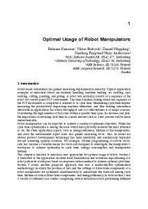
Fig. 1 For the DLR Justin manipulator (a), a skeleton can be found (b) by considering the axes of the arms and the spine of the torso. Segments are drawn between the Cartesian positions of some crucial joints.
management of possible discontinuities, fast Jacobian computation via symbolic description and its consequences.
2 Whole-Body Modelling with the Skeleton Algorithm As briefly introduced, an approach which automatically selects a control point on a whole kinematic structure, based on sensor information and analytical computation, is useful for pHRI applications. In addition, the control points should be computed fast, based on a model of the environment which leads to simple distance computation and trajectory determination. These considerations lead to the so-called “skeleton algorithm” developed for collision avoidance applications (see [4] and references therein) whose steps include: building a proper model of the robot, namely the skeleton, useful for analytical computation; finding the control points along the skeleton, via distance computation or explicit user’s decision; generating trajectories and corresponding joint commands for the controller.
2.1 Skeleton-Based Modelling The problem of analyzing the whole volume of the parts of a manipulator is simplified by considering a skeleton of the structure, and proper volumes surrounding it. With reference to the DLR Justin manipulator [3], such a skeleton is reported in Figure 1.
Inverse Kinematics of Robot Manipulators with Multiple Moving Control Points
431
If segments are built that “span” the kinematic structure of a manipulator (see Figure 1), its whole shape can be modelled. The underlying idea is that a solid of revolution can express the shape of a link, but this can be partially modified using properly the distance functions from every point of the link, resulting in a bounding volume around the point. These multiple volumes form a virtual region which has to approach the real volume of the considered part of a manipulator. Automatic skeleton building from Denavit–Hartenberg (DH) parameters is possible. In fact, a standard DH table gives the possibility of computing the Cartesian position of each joint. These positions can constitute the ends of the segments of the skeleton (nodes), and some of these possible nodes will be discarded if they coincide with other nodes already present in the skeleton. It is important to consider segments which cover the spine of all the mechanical parts: this has a reflex on DH tables when manipulator links have parts on both sides of a revolute joint as, e.g., for counterbalances or for allocating motors. Building the skeleton, the focus is then on distance evaluation from the segments on the robot (bounding volumes) to the environment: this is the basis for motion control in an unstructured domain. The complete environment has to be modelled with geometric figures. In the design of the skeleton, some heuristics can help in discarding useless computation; nevertheless, the general case of computing all possible distances between simple objects like segments, regions of a plane (circles, rectangles) or points has the only limit of the time complexity for modelling the whole operation environment. The distances between these simple objects can be obtained via analytical formulas [5].
3 Inverse Kinematics with Multiple Control Points Every point on the structure can be considered a control point, identified by a set of DH parameters. The proposed symbolic approach is based on the consideration that, if one considers a manipulator and its direct kinematics equation, changing the value of its DH parameters results in the kinematics equations of another manipulator, whose end-effector is located before the real end-effector: that is equivalent to moving the control point of the structure. In detail, since control points always lie on the spine of the robot links, the direct kinematics and the Jacobian computation can be carried out in a parametric way for a generic point p i , which is located after the i-th joint. Considering the homogeneous transformation relating the (i − 1)-th frame (corresponding to the i-th joint) to the next frame, by simply replacing the DH parameter corresponding to the link length with the distance to the considered control point, a new “shorter” manipulator is considered for control. The values of direct kinematics and Jacobian for the specified control point have then to be considered by setting to 0 the DH values corresponding to frames located below the control point in the kinematic chain. If the
432
A. De Santis and B. Siciliano
displacements on the links vary continuously and sequentially, from the tip of the robot towards the base and vice versa, the whole skeleton can be spanned. In order to generate proper reference motion for the control points, in general, potential fields or different techniques can be used in order to generate the forces or velocities which will produce the desired motions. In [4] it is discussed how, e.g., repulsion forces can be derived from a potential function. These forces can be naturally used to compute avoidance torques at the manipulator joints via the Jacobian transpose. Nevertheless, it should be pointed out that suitable repulsion velocities could be likewise generated in lieu of forces. The interesting implementation in velocity control will be presented, since the differential kinematics equation has an important modification, due to the fact that not only the joint angles, but also other kinematic parameters in the DH table may change during the task. The additional suggested tools for a velocity-level implementation are the choice of a modular Jacobian, and the proper management of a moving control point.
3.1 Modular Jacobian The need for a modular Jacobian comes from the number of matrix multiplications which are necessary for an arbitrary number of degrees of freedom (DOFs). For the purpose of control, the Jacobian matrix is the cornerstone: similarly to the previous discussion, a symbolic Jacobian can be used, where the kinematic parameters in the DH table change as described above, allowing the motion of the control point. The dimensions of such a matrix change, depending on the available DOFs before the control point. The crucial aspect is that derivation of the differential kinematics equation is affected by the motion of the multiple control points. This can be also taken into account in a symbolic expression, as discussed below.
3.2 Differential Kinematics with Moving Points Considering the direct and differential mappings with the standard DH parameters, the usual differential kinematics equation does not take into account the possibility of varying those kinematic parameters other than joint values. A complete model is as follows. The direct kinematics equation can be written in the form pi = k(q i )
(1)
where the vector q i contains the vectors of the standard DH variables d i , a i , θ i , α i . The differential mapping, discarding possible variations of the values in α i , is therefore
Inverse Kinematics of Robot Manipulators with Multiple Moving Control Points
p˙ i =
433
∂k ∂θ i ∂k ∂a i ∂k ∂d i dk = + + dt ∂θ i ∂t ∂a i ∂t ∂d i ∂t
= J θ,i (θ i , a i , d i )θ˙ i + J a,i (θ i , a i , d i )a˙ i + J d,i (θ i , a i , d i )d˙ i .
(2)
Given a control point pi , the matrices J a,i and J d,i in (2) are the Jacobians which express the contribution to the motion of the control point of the variations of the DH values which characterise the control point. Moreover, θ i expresses the vector of the joint values which contribute to the motion of the control point. Notice that J θ,i is the ordinary Jacobian up to the control point, for a given set of DH parameters. There are proper ways [6] for reducing the number of nonnull values in the d i and a i vectors of DH parameters. Often, this is intrinsically forced by the manipulator’s design. As a simple case, consider a manipulator kinematics where only some values in the vector d i change. In this situation, the way to compute the joint variables for a moving point on the skeleton of the robot is the following: θ˙ i = J †θ,W ,i (p˙ i − J d,i (θ i , a i , d i )d˙ i )
(3)
where the subscript W for the pseudoinverse of the Moore–Penrose Jacobian matrix J †θ,W,i (corresponding to the control point p i ) is referred to possible joint involvement weighing. Based on these simple modifications, multiple-point control, which has shown to be central in interaction with robots, can be accomplished easily both in force and velocity control. The main issue is that the control points, with the associated Jacobian, move on the robot; therefore, this motion is taken into account in the differential kinematics.
3.3 Continuity of Moving Control Points When a control point is computed automatically, e.g., via distance evaluation from the closest obstacle (or goal) to the skeleton of the manipulator, there is the possibility that its position changes in a discontinuous fashion. Consider as an example the case of multiple obstacles approaching an articulated robot. Moreover, some heuristics or the need for a reduced number of control points can result in some sudden change of control point, and therefore of the corresponding DH values. In order to avoid this problem, the DH values for the control point have to be forced to vary with continuity and in the right sequence: this corresponds to moving to the next control point always lying on the skeleton. This can achieved, e.g., via spline interpolation resulting in moving the current control point towards next node of the skeleton, and then from there to the new control point, via a sequence of Cartesian positions of the joints, i.e., the nodes of the skeleton [5]. The sequence of variation of the DH parameters is important for simulating such a motion on the spine of the links, and the use of spline interpolation is suggested for specifying values of the higher-order derivatives of DH values.
434
A. De Santis and B. Siciliano
(a)
(b)
(c)
Fig. 2 The control point (small circle) on the skeleton, automatically computed as the closest to a moving object (big circle), can give a discontinuity to reference trajectories, moving abruptly on a new segment.
In order to reach the new control point via interpolation, a delay is to be considered before the change of the control point is performed. This delay has to be compatible with parameters related to the current motion of the robot such, e.g., the time-to-collision. The possibility of smoothly moving the control point is useful also for forcing its motion on the skeleton in case of distance computation between parallel segments, where the computed closest point can move abruptly from an end to the other of the segment of the skeleton, in case of motion of an obstacle segment passing through a configuration which results in a parallelism with respect to the segment on the manipulator’s skeleton. Both first- and second-order inverse kinematics schemes [7] can be easily modified for taking into account the presence of the moving control point with variable kinematic parameters. In the case of second-order algorithms, the derivatives of the additional Jacobian matrices which have been introduced have to be computed also. With reference to Figure 2, it can be seen that a single control point which is automatically computed as the closest to a collision, based on environment modelling, can move abruptly on the articulated structure. The use of different filters for the motion on the control point depends on the control algorithm too: if the control uses higher order derivatives of the position, motion has to be smooth enough to ensure continuity of these data. Figure 3 shows an example of variation of the DH parameters which identify the control point for a three-link planar manipulator, whose lengths are 0.4 m, 0.3 m, 0.2 m. In such a manipulator, only the values in the vector a i , i.e., ai (1), ai (2), ai (3), change for a control point p i on the skeleton. If the control point moves from the middle of the first link (p 1 ) to the middle of the third link (p2 ), the resulting continuous and sequential change in the DH parameters, obtained via cubic spline
Inverse Kinematics of Robot Manipulators with Multiple Moving Control Points
435
0.45
0.8
0.4
0.7
p
0.6
0.35
a i(1)
2
0.3 0.5
[m]
0.25 0.4
0.2 0.3 a (2)
0.15 0.2
p1
0.1
0
i
0.1
0
0.1
a i(3)
0.05
0.2
0.3 [m]
0.4
0.5
0.6
(a)
0 0
0.05
0.1
0.15
0.2
0.25
0.3
0.35
[s]
(b)
Fig. 3 When a control point’s position is expected to change, e.g. from p1 to p2 (a), the desired new DH parameters are to be reached sequentially and with continuity (b).
interpolation, is reported. The time for reaching the desired final value for each parameter has been set always equal to 0.1 s. This time interval is a parameter for the spline interpolator. In this case, the change of three parameters results in reaching control point after 0.3 s. Meanwhile, the control point is moving on the skeleton and its motion is taken into account as described above.
4 A Simulation Case Study A short example is here reported for simplicity. Consider the case of a 3-link planar manipulator approaching an object located in the position pg . If one just wants that the robot hits the object, the closest point on the object from p g , i.e., the point p c , has to be attracted. Inverse kinematics can be performed as introduced for a single moving control point, which has to be driven towards pg . A velocity is commanded which is proportional to the difference between pg and p c . When the manipulator moves, if p c is automatically computed as the closest to the goal point, its desired location may change abruptly from one link to the other (see Figure 3). For the � �T simulations, the length of each link is 0.2 m, the goal position is p g = 0 −0.2 , and the motion of the control point is limited to the last two links. In order to smoothen the change of control point’s position, a spline interpolation for the DH values of pc is used. This results in a sliding motion of the control point pc on the manipulator up to the new desired one. The resulting Cartesian motion and joint motions corresponding to the moving pc is reported in Figure 4. Notice that a damped-least-squares solution has been adopted in the pseudoinversion of the
436
A. De Santis and B. Siciliano
0.5 0.4
y
0.3 0.2 0.1 0
0
0.2 x
0.4
(a)
2 θ2
1.5 1 [rad]
0.5
θ3
0 −0.5 −1
θ1
−1.5 −2
1000
2000
3000 [ms]
4000
5000
(b) Fig. 4 (a) Time history of the Cartesian motion of control point (thick line) and end-effector (thinline): notice that the control point moves soon to the new desired value. (b) Joint motion in the proposed case study.
Jacobian matrix; notice also that, in the final part of the trajectory, the desired direction for the control point is unfeasible (singular direction). These two last remarks are reported for suggesting the need for more global approaches including proper trajectory planning, in order to avoid local minima during the motion. As a simple example, the desired velocity for reaching the goal point pg can be interpolated for avoiding high speeds in the first part of the motion. From Figure 5 it is possible to observe the progressive modification of the values in the a c vector (according to the notation introduced in Section 3.2), corresponding
Inverse Kinematics of Robot Manipulators with Multiple Moving Control Points
437
0.2 a2
[m]
0.15
0.1
0.05 a
3
0 0
50
100
150 200 [ms]
250
300
Fig. 5 Time history of the values in the vector a.
to the motion of p c , which is initially located at the end-effector (default) and then moves to the second link. Notice that the desired positions of pc during the simulations are reached after fixed time slots, specified for the spline interpolators. During this time, no additional new desired points are computed. If the control point does not change any longer, the scheme coincides with the well-known closed-loop inverse kinematics (CLIK) with no feedforward of velocity.
5 Conclusion An approach to inverse kinematics for possibly moving control points on the kinematic chain of a robot manipulator has been introduced in this paper. It is based on whole-body modelling: analytical computation or explicit choice may be used for setting the control points. Such control points are forced to move smoothly on the spine of the links of the considered robot manipulator. Simulation results have been provided for a simple planar robot manipulator; future work will be aimed at testing the approach on spatial manipulators, such as the DLR Justin manipulator.
Acknowledgements This work is partly a development of a research started when the first author was a visiting researcher at DLR, supervised by Dr. Alin Albu-Schäffer. This work was supported by the PHRIENDS Specific Targeted Research Project, funded under the 6th Framework Programme of the European Community under Contract IST– 045359. The authors are solely responsible for its content. It does not represent the
438
A. De Santis and B. Siciliano
opinion of the European Community and the Community is not responsible for any use that might be made of the information contained therein.
References 1. De Santis, A., Siciliano, B., De Luca, A. and Bicchi, A., An atlas of physical Human–Robot Interaction, Mechanism and Machine Theory 43, 253–270, 2008. 2. De Santis, A., Pierro, P. and Siciliano, B., The virtual end-effectors approach for human-robot interaction, in Advances in Robot Kinematics: Mechanisms and Motion, J. Lenarˇciˇc, B. Roth (Eds.), Springer, pp. 133–144, 2006. 3. Ott, C., Eiberger, O., Friedl, W., Bäuml, B., Hillenbrand, U., Borst, C., Albu-Schäffer, A., Brunner, B., Hirschmüller, H., Kiehlöfer, S., Konietschke, R., Suppa, M., Wimböck, T., Zacharias, F. and Hirzinger, G., A humanoid two-arm system for dexterous manipulation, in Proceedings 2006 IEEE International Conference on Humanoid Robots, Genova, I, IEEE, pp. 276–283, 2006. 4. De Santis, A., Albu-Schäffer, A., Ott, C., Siciliano, B. and Hirzinger, G., The skeleton algorithm for self-collision avoidance of a humanoid manipulators, in Proceedings 2007 IEEE/ ASME International Conference on Advanced Intelligent Mechatronics, Zürich, Switzerland, IEEE, 2007. 5. De Santis, A., Modelling and Control for Human–Robot Interaction, Research Doctorate Thesis, Università degli Studi di Napoli Federico II, Italy, 2007. 6. Sciavicco, L. and Siciliano, B., Modelling and Control of Robot Manipulators, 2nd edition, Springer-Verlag, London, UK, 2000. 7. Caccavale, F., Chiaverini, S. and Siciliano, B., Second-order kinematic control of robot manipulators with Jacobian damped least-square inverse: Theory and experiments, IEEE/ASME Transactions on Mechatronics 2, 188–194, 1997.