AbstractâIn large scale Internet of Things (IoT) systems, statistical analysis is a crucial technique for transforming data into knowledge and for obtaining overall ...
2013 IEEE International Conference on Green Computing and Communications and IEEE Internet of Things and IEEE Cyber, Physical and Social Computing
IOT-StatisticDB: A General Statistical Database Cluster Mechanism for Big Data Analysis in the Internet of Things
Zhiming Ding, Xu Gao, Jiajie Xu, and Hong Wu Institute of Software, Chinese Academy of Sciences Beijing 100190, P.R.China {zhiming, gaoxu, jiajie, wuhong}@iscas.ac.cn such general information is far more important than the individual sampling values collected from the sensors. Another example is traffic flow analysis through GPStracked vehicles (or “moving objects”). Each moving object can sample its motion vectors (including location, speed, and direction) repeatedly through GPS and send them to the data center. However, a motion vector can only reflect the status of a certain vehicle at a certain time instant. To get the traffic flow information of the whole traffic network, statistical analysis should be conducted based on huge numbers of motion vectors. There are many existing works which can be used for statistical analysis on sensor sampling data. However, most of them are implemented outside the database kernel, and focus on the specialized analytic methodologies [1-4], making them unsuited for the IoT environment where both the data types and the statistical queries are heterogeneous and diverse. For instance, in a modern intelligent transportation system, there could be many different kinds of sensors which can collect raw data for traffic flow analysis, like loop sensors, traffic video cameras, GPS sensors, RFID readers, optical sensors, microwave vehicle detectors, and so forth. The sampling data of these sensors have totally deferent formats and semantics. Therefore, each kind of sensors needs a different statistical analysis module, which could be a heavy workload for system developers. On the other hand, if we support generalized statistical analysis in database kernel level, then complicated statistical analysis can be easily expressed in the standard SQL interface. Another limitation for existing statistical analysis methods is that most of them are centralized solutions [510], which are unsuited for big data analysis. For instance, the most effective clustering algorithms, DBSCAN [6], OPTICS [7], BIRCH [8], K-Means and its variations [9-10], are all designed for centralized data analysis environments and can not be directly used in distributed and parallel environments. Besides, a lot of index methods to speed up the statistical analysis are not suited for the IoT environment because the frequent data updates can cause very high index update costs. There are several database management systems which can support statistical analysis on structured data [11-13]. However, only simple statistical functions (like average,
Abstract—In large scale Internet of Things (IoT) systems, statistical analysis is a crucial technique for transforming data into knowledge and for obtaining overall information about the physical world. However, most existing statistical analysis methods for sensor sampling data are implemented outside the database kernel and focus on specialized analytics, making them unsuited for the IoT environment where both the data types and the statistical queries are diverse. To solve this problem, we propose a General Statistical Database Cluster Mechanism for Big Data Analysis in the Internet of Things (IOT-StatisticDB) in this paper. In IOT-StatisticDB, statistical functions are performed through statistical operators inside the DBMS kernel, so that complicated statistical queries can be expressed in the standard SQL format. Besides, statistical analysis is executed in a distributed and parallel manner over multiple servers so that the performance can be greatly improved, which is confirmed by the experiments. Keywords - Statistical Database, Internet of Things, Big Data, Sensor Sampling Data, Spatial-Temporal Data.
I. INTRODUCTION With the recent advances in sensor networks and in the Internet of things (IoT), statistical analysis of massive sensor data becomes a key research issue. In a large scale IoT system, there are numerous sensors and / or monitoring devices connected, which repeatedly send sampling data to the data center. The data center not only needs to store, manage, and query the individual sampling data efficiently, but also needs to conduct statistical analysis in order to extract more general information about the physical world. Such a scenario is a typical big data environment because of the huge volume of data and high frequency of updates. As a result, a lot of challenging problems need to be solved. Statistical analysis of sensor sampling data is one of the most important procedures in IoT systems in order to transform “data” into “knowledge”, and is crucial in a lot of applications like disaster monitoring, emergency management, e-health, intelligent transportation systems, and so forth. As an example, let’s consider the pollution monitoring in a large city. Each pollution sensor can only monitor a small area, and only through statistical analysis we can get more general information over large areas such as “what is the most polluted region of the city”, and “how the most polluted region changes over time”. It is obvious that 978-0-7695-5046-6/13 $26.00 © 2013 IEEE DOI 10.1109/GreenCom-iThings-CPSCom.2013.104
535
min, max, and count) can be supported while spatialtemporal statistical analysis and network-based analysis on large-scale sensor sampling data can not be supported. It is thus critical to investigate the database kernel level, parallel statistical analysis techniques for massive sensor sampling data in the Internet of Things. Under the framework of IoT database cluster, we seek to design some general statistical operators that can be used in SQL such that the complicated statistical analysis requirements can be easily expressed in a generalized manner. In this way, the application designers and the system developers can work collaboratively in different layers, which can significantly improve the efficiency of IoT system development. However, according to literature analysis, there is no existing work in this direction. To solve the above problems, we propose a General Statistical Database Cluster Mechanism for Big Data Analysis in the Internet of Things (“IOT-StatisticDB” for short) in this paper. The remaining part of this paper is organized as follows: Section 2 describes the architecture, the data types, and operators of IOT-StatisticDB, Section 3 presents the parallel statistical analysis methods of IOTStatisticDB, Section 4 discusses implementation issues and performance evaluation results, and Section 5 finally concludes the paper.
analysis methods, designed as statistical analysis operators, as shown in Table 1. TABLE I.
CLASSIFICATION OF STATISTICAL ANALYSIS METHODS IN IOT-STATISTICDB
Euclidean-Based Network-Based
Spatial Aggregation
Parameter Aggregation
spatialAggrEU spatialAggrNet
parameterAggrEU parameterAggrNet
Suppose that we have various kinds of sensor sampling data about Beijing. Euclidean-based spatial aggregations can answer queries like “What is the geographical area in Beijing with air pollution index exceeding the threshold �=300 currently?” (the output of the query is a spatial region with hole, as illustrated in Figure 1), while networkbased spatial aggregations can answer queries like “Tell me the road sections where the vehicle speed is slower than 5 km/h in the WestBeijing area at time t”. Output of the statistical query
Air Pollution Index
II. ARCHITECTURE OF IOT-STATISTICDB AND THE DATA TYPES AND OPERAORS FOR STATICAL ANALYSIS Architecture of IOT-StatisticDB In many applications like environment monitoring, we need to conduct complex statistical analysis to understand the physical world and to explore useful knowledge based on the IoT sampling data. We should notice that many applications require similar or even the same statistical operations at the database level. This observation motivates us to propose a database kernel level statistical analysis mechanism to support high performance common analytics on IoT sampling data. Among the complex statistical analysis operations in demand, we classify some typical ones and implement uniform operators for them. In general, most of the statistical operations in IoT systems can be classified into spatial aggregations and parameter aggregations. For a given data set, spatial aggregations can cluster the geographical values extracted from sensor data to larger groups so that meaningful knowledge about spatial distributions can be extracted. On the other hand, parameter aggregations allow us to get aggregation information like average, minimum, maximum, and count from the sensor sampling values. In addition, both parameter aggregations and spatial aggregations can be further divided into Euclidean-based and network-based. Euclidean-based aggregations do not consider traffic networks while network-based aggregations take the underline traffic networks into account. Therefore, in IOT-StatisticDB, we can have 4 kinds of statistical
600 300 41.2 0 115.4 115.73 116.17
40.8 40.4 116.4
40 116.73 117.17
A.
39.6 117.4 39.2
Figure 1. Euclidean-based Spatial Aggregation
Example Euclidean-based parameter aggregation queries include “What is the average PM2.5 level in Beijing at time t”, and network-based parameter aggregations can answer queries like “Tell me the traffic parameters of every road section in West Beijing”. Network-based parameter aggregations compute the traffic parameters of each road section of a given area by analyzing the GPS trajectories of moving objects or by analyzing the sampling data of traffic flow sensors. To support IoT data statistical analysis efficiently, we adopt a three-layered architecture in IOT-StatisticDB, as shown in Figure 2.
Sampling Recerver
Master Server
IoT-Storage and Statistics Layer
Node Servers Raw Data Storage
Raw Data Storage
Raw Data Storage
Raw Data Storage
Raw Data Storage
Raw Data Storage
IoT-Raw Data Storage Layer
Sersor and Monitoring Device Layer Traffic Sensors Hydrological Sensors
Geological Sensors
Video Monitors
Telemetric Monitors
GPS Sensors
Figure 2. Architecture of IOT-StatisticDB
536
As shown in Figure 2, the sensor and monitoring device layer includes various kinds of sensors and /or monitoring devices (multimedia monitoring devices plus the corresponding vitalization [14] modules are equivalent to sensors, so that they are uniformly called sensors in this paper). All the sampling values (including numeric values and multimedia values) generated from this layer are sent to and kept at the IoT-raw data storage layer. These values can be organized in key-value stores (like Cassandra, MangoDB, and so forth) by taking sensor identifiers as the key. Since data are sampled densely, not all samplings need to be stored at the IoT-storage and statistics layer. Only key sampling values (for numeric sensors) and vitalized values (for multimedia devices) are kept at this layer. The IoT-storage and statistics layer is the key for multimodal data query processing (like spatial-temporal queries, keyword-based queries, and value-based approximate queries) and for statistical analysis. In the following two subsections, we describe the working mechanism of this layer, including the data types and the related operators for storing and analyzing the IoT data.
SamplingValue = (t, loc, npos, schema, value) where t Instant is the sampling time, loc Point is the sampling location, npos String is the network position of the sampling (expressed with an edge identifier, and set to null if not on road network), schema String and value String denote the format and the actual value of the sampling respectively. Through the SamplingValue data type, we can express heterogeneous sensor sampling value in a uniformed manner. Table 2 shows some examples. TABLE II. EXAMPLES OF SENSOR SAMPLING VALUES
Type of Sensor Temperature Sensor GPS Sensor Wind Sensor Vitalized value from Traffic Video Camera
Sensor Sampling Value (t1, (39.5, 145.2), null, “temperature: real”, 27.5) (t2, (39.3, 144.3), e201, “speed: real, direction: real”, (62.5, 22)) (t3, (38.2, 142.8), null, “windspeed: real, winddir: real”, (62.5, 22)) (t4, (39.7, 142.1), e202, “averageSpeed: real, jam: bool”, (62.5, true))
A sampling value can have multiple components. For instance, the GPS sampling value has 2 components: speed (62.5) and direction (22) (node that longitude and latitude are expressed in loc instead of as components). Components of a sampling value can be expressed through the Sampling Value Component data type. Definition 3 (Sampling Value Component) A sampling value component, denoted as SamplingComponent, can be defined as follows: SamplingComponent = (cSchema, cValue) where cSchema and cValue are the schema and the value of the component respectively. For instance, the two components of the GPS sampling value in Table 2 are expressed as (“speed: real”, 62.5) and (“direction: real”, 22) respectively. Definition 4 (Sampling Sequence) For a certain sensor, its sampling sequence, denoted as SamplingSequence, is composed of all sampling values from the sensor for a certain time period, ordered by sampling time, and can be expressed as follows:
B. Data Storage and Distribution at the IoT-Storage and Statistics Layer As shown in Figure 2, the IoT-storage and statistics layer assumes a 2-layered structure. The master server is the coordinator which only keeps global catalogs and global indices, while the node servers store the key sampling values sent from the IoT-raw data storage layer. All key sampling values are sent to the sampling server first, which then distributes them to the corresponding node servers according to their sampling locations. In this subsection, we first describe how traffic network and sampling values are expressed at the IoT-storage and statistics layer of IOT-StatisticDB, and then discuss how they are distributed among multiple servers. Definition 1 (Traffic Network) A traffic network, Net, is defined as follows: Net = (E, N) where E is a set of directed edges and N is a set of nodes. A direct edge (or simply edge) e E is defined as the form e = (eid, geo, len, nids, nide), where eid String is the identifier of e; geo = (p1, p2, …, pn) Polyline is the geometry of e where pi (1d i d n) Point is the ith vertex of the polyline; len Real is the length of e, and nids, nide String are the identifiers of the starting and ending nodes which are connected by edge e. A node n N is defined as the form n = (nid, loc,
n
SamplingSequence=(schema, (ti, loci, nposi, valuei, flagi) i 1 ) where schema is the format of the sampling values; ti, loci, nposi, valuei are the time, location, the network position, and the actual value of the ith sampling respectively; and flagi indicates whether the ith sampling value is a “breaking point” in the sequence. For static sensors, as their loc attribute is a constant value, we can further simplify their SamplingSequence format as:
m
(eidi) i 1 , mat), where nid String is the identifier of n; loc Point is the location of n; eidi (1d i d m) String is the identifier of the ith edge connected by n; and mat is the connectivity matrix of n, which describes the traffic transferability among different edges through the node [15]. Definition 2 (Sampling Value) A sampling value, denoted as SamplingValue, is defined as follows:
n
SamplingSequence=(schema,loc,npos,((ti,valuei, flagi)) i 1 ) Above two different formats for sampling sequences can be differentiated by the database automatically.
537
In implementation, the SamplingSequence data type can be designed and implemented as a pointer in the tuple leading to a file block where the real data are stored. In this way, data updates triggered by new samplings can be conducted quickly without database updates involved. With the above data types, we can create the following table for storing sensor sampling data:
C. Query Operators for Data Retrieval and for Statistical Analysis at the IoT-Storage and Statistics Layer The data types allow us to express sensor sampling data and the underlying traffic network in databases and in file systems. To query the sensor data and to conduct statistical analysis, we need to further define a set of operators so that complicated statistical functions can be expressed in SQL. In defining operators, we use signatures which describe the input and the output data types of the operators [15]. In general, the operators in IOT-StatisticDB can be divided into the following 4 categories.
CREATE TABLE IoTData (SensorID: String, SensorType: String, DeployedBy: String, DepoyedTime: Instant, Samplings: SamplingSequence)
where SensorID, SensorType are the identifier, the type (e.g. VehicleGPS, RFID, etc.) of the sensor; DeployedBy and DeployedTime are the deplorer and time of the deployment; SamplingSquence is the sampling sequence from sensors. Traffic network is not stored as relational tables. Instead, it is directly stored in file system. To speedup the data access, indices are built on traffic network. In the following, we discuss how the sampling data and the traffic network are distributed among the master server and the node servers. In the IoT-storage and statistics layer, sampling data are distributed at the node servers according to their geographical attribute. Each node server node corresponds to a spatial area �(node), which is called the service area of node. Any two service areas do not intersect each other and the union of all services areas is equal to the whole application area G. Therefore, the service areas actually make a spatial partition of G. For any sampling value v = (t, loc, npos, schema, value), if v is from a static sensor, then the sampling receiver simply transfers it to the node server whose service area contains loc. If v is from a mobile sensor (like GPS sensor), the sampling receiver needs to conduct necessary interpolations at the border of service areas, and sends the resultedvalues to the corresponding node server(s), as shown in Figure 3.
(1) Truncation Operators on Sampling Sequences truncateGeo returns part of sampling sequence which is inside a given region spatially, while truncateTime returns part of the sampling sequence which is inside a given time period temporally. atInstant computes and returns a sampling value corresponding to a specified time instant t. If t is not a sampling time, then necessary interpolation is required. The signatures of these operators are as follows: truncateGeo:SamplingSequenceuRegion o SamplingSequence truncateTime:SamplingSequenceuPeriodsoSamplingSequence atInstant:SamplingSequence u Instant o SamplingValue
(2) Projection Operators Projection operators can be further divided into sampling-sequence-based and sampling-value-based. Sampling-sequence-based projection operators include sProjectLines, sProjectPoint, and sProjectNetPos, which project a sampling sequence towards the spatial plane, and sProjectTime which project a sampling sequence towards the temporal axle. Their signatures are as follows: sProjectLines: SamplingSequence o Lines //for moving sensors sProjectPoint: SamplingSequence o Point //for static sensors sProjectNetPos: SamplingSequenceo Set(String) sProjectTime: SamplingSequence o Periods
Sampling-value-based projection operators include vProjectPoint and vProjectNetPos which get the sampling value’s sampling location and the corresponding network position respectively, and vProjectTime which get the sampling value’s sampling time. Their signatures are as follows:
Master Node
node1
node2
node3
node4
Node Servers
t
vProjectPoint: SamplingValue o Point vProjectNetPos: SamplingValue o String vProjectTime: SamplingValue o Instant
breaking points locations of sampling values Service Areas �(node2)
�(node1) �(node4)
(3) Component Extraction Operator The getComponent operator returns the ith component of a sampling value, and its signature is:
�(node3)
getComponent:SamplingValueuintegeroSamplingComponent
(4) Statistical Analysis Operators There are 4 statistical operators as introduced in Table 1. Their signatures are as follows:
Figure 3. Data Distribution at the IoT-Storage and Statistics Layer
The traffic network is also distributed among the node servers. Node server node only keeps the edges and the nodes which are inside or intersect �(node). For the sake of efficiency, the master server needs to store the whole traffic network.
spatialAggrEU: String u String o Region spatialAggrNet: String u String o Lines parameterAggrEU: String u String o Real parameterAggrNet: String u String o Set(String u String)
538
Each statistical operator has two input strings. The first input string is an SQL statement which collects statistical raw data, while the second input string specifies a statistical method and its parameters. For example:
points into a region, and sends the final result to the master server, as shown in Figure 4. �(node2)
�(node1)
Let Q = “SELECT sProjectPoint(Samplings) FROM IoTData WHERE SensorType = “PM25Sensor” AND inside(ssProjectPoint(Samplings), BeijingGeo) AND getComponent(aatInstant(Samplings, t), 1) > 350”
Output region of statistical query
BeijingGeo
Select spatialAggrEU(Q1, “DBScan(distance1, number1)”) �(node3)
The output of the above query is a Region value, which corresponds to the spatial area with PM2.5 level over 350 at time t. Let’s see another example:
Output points of Qdata
�(node4)
Figure 4. Euclidean-Based Spatial Aggregation
When all the participating node servers have returned the query results, the master server needs to merge the results and returns the final result to the querying user. Algorithm 1 describes the processing of the EuclideanBased Spatial Aggregation operator.
Let Q = “SELECT getComponent(aatInstant(Samplings, t2), 1) FROM IoTData WHERE SensorType = “TrafficSensor” AND inside(ssProjectPoint(Samplings), BeijingGeo)”; Select parameterAggrNet(Q, TrafficSensorAnalysis);
Algorithm 1. Processing of the spatialAggrEU(Qdata, cMethodPara) operator
The output of this query is a set of (edgeID, para) pairs, where para is a structured string describing the traffic parameters of edge edgeID, including average speed, traffic jam status, flux, number of vehicles, and so forth.
INPUT: Qdata: String; // Statistical raw data collection query cMethodPara: String; // Clustering method and its parameters; OUTPUT: R: Region;
III. PARALLEL STATISTICAL ANALYSIS ALGORITHMS IN IOTSTATISTICDB
queryRegion = GetQueryRange(Qdata); Nodes = {node | area(node) queryRegion � Ø} FOR node Nodes DO IN PARALLEL StatisticalRawData = Execute(Qdata); R (node) = clusterContour(StatisticalRawData, cMethodPara); 6. SendMaster(R (node)); 7. ENDFOR; 8. Results = {R(node) | node Nodes}; 9. R = regionMerge(Results); 10. Return (R).
1. 2. 3. 4. 5.
In IOT-StatisticDB, all queries are sent to the master server first, which then conducts global execution of the query by coordinating multiple node servers for parallel execution. In this section, we describe the parallel processing mechanism for statistical queries in IOTStatisticDB. A. Euclidean-Based Spatial Aggregation The Euclidean-based spatial aggregation operator takes the form spatialAggrEU(Qdata, cMethodPara) where Qdata String is an SQL statement which collects the statistical raw data and cMethodPara specifies the clustering method and its parameters. The output of the operator is a region. As an example, let’s consider the following query: [Query Q1] Query the area in BeijingGeo where the pollution level is above 450 at time t.
Algorithm 1 first gets the query range queryRegion through the GetQueryRange(Qdata) function, then all node servers whose service areas intersect with queryRegion execute the statistical analysis in parallel. Each related node server first executes Qdata (line 4) to get statistical raw data, and then calls the clustering procedure specified by cMethodPara to cluster the raw data and outputs the contour of the clusters (which is a region value) (line 5), and then sends the result to the master server (line 6). After the master server receives the feedback from all related node servers, it merges the feedbacks into one region through the regionMerge function (lines 8, 9) and returns the final result to the querying user (line 10).
Let Qdata = “SELECT sProjectPoint(Samplings) FROM IoTData WHERE SensorType = “PollutionSensor” AND inside(ssProjectPoint(Samplings), BeijingGeo) AND getComponent(aatInstant(Samplings, t), 1) > 450”; Select spatialAggrEU(Qdata, DBScan(distance1, number1))
When receiving the above query, the master server first sends the query to all node servers whose service areas intersect with the query range BeijingGeo. After a node server receives the above query, it first executes Qdata to collect the statistical raw data, and the result is a set of points. Then it calls the DBScan algorithm (with distance1, number1 as parameters) to cluster the
B. Network-Based Spatial Aggregation Network-based spatial aggregation is similar to Euclidean-based spatial aggregation. The main difference is that the clustering method takes traffic network as the clustering center and the output is a Lines value instead of a
539
Region value (note that a Lines value may contain multiple polylines [15]). As an example, let’s consider the following query: [Query Q2] Query the blocked edge sections (with vehicle speed lower than 5 km/h) at time t in the traffic network of Beijing area (in side the region BeijingGeo).
queryRegion = GetQueryRange(Qdata); Nodes = {node | area(node) queryRegion � Ø} FOR node Nodes DO IN PARALLEL StatisticalRawData = Execute(Qdata); R (node) = netClusterLines(StatisticalRawData, trafficNet, cMethodPara); 6. SendMaster(R(node)); 7. ENDFOR; 8. Results = {R(node) | node Nodes}; 9. R = linesMerge(Results); 10. Return (R). 1. 2. 3. 4. 5.
Let Qdata = “SELECT atInstant(Samplings, t) FROM IoTData WHERE SensorType = “VehicleGPS” AND inside(ssProjectPoint (aatInstant(Samplings, t)), BeijingGeo) AND getComponent(aatInstant(Samplings, t), 1) < 5”
Algorithm 2 is similar to Algorithm 1. The main difference is that the clustering method, netClusterLines, need to use the traffic network to get the output (line 5), and the merging is line-based (line 9).
Select spatialAggrNet(Qdata, DBScanNet(distance1, number1))
In processing this query, the master server first sends the query to the node servers whose service areas intersect the query range BeijingGeo. For each related node server, it first executes the data collection query Qdata which outputs a set of sampling values at time t which satisfying the query condition. For a certain sampling sequence samplings, atInstant(Samplings, t) computes the sampling value corresponding to time t, and the output sampling value includes the location, the speed, and the direction of the corresponding moving object at time t, as shown in Figure 5. �(node1)
C. Euclidean-based Parameter Aggregation The Euclidean-based parameter aggregation operator, parameterAggrEU, can be used to compute the aggregation of a set of raw values, such as average, min, max, and count. Let’s consider the following example: [Query Q3] Query the average pollution level at time t in BeijingGeo. Let Qdata=“SELECT getComponent(aatInstant(Samplings, t), 1) FROM IoTData WHERE SensorType = “PollutionSensor” AND inside(ssProjectPoint(Samplings), BeijingGeo)”;
�(node2)
edge4
edge7
edge6 edge3
edge1 edge8 edge5 �(node3)
Select parameterAggrEU(Qdata, Average)
Output of Qdata
When processing this query, the master server first sends the query to all the node servers whose service areas intersect with the query range BeijingGeo. Each related node server first executes the statistical raw data collection query Qdata, whose result is a set of pollution level values. Then, the node server computes the average of the raw data, and sends the pair (average, number), where average is the average of the raw data and number is the number of raw data, to the master server for merging. The merged final result is sent to the querying user. The general format of the Euclidean-based parameter aggregation operator is parameterAggrEU(Qdata, method). Depending on the aggregation method specified by method, the master server adopts different merging methods. Suppose that the feedback is: (�1, �1), (�2, �2), … (�n, �n). If method = “average”, the merging result R can be computed as follows:
edge2 �(node4)
Figure 5. Network-Based Spatial Aggregation
Then, the node server calls the network-based clustering method, DBScanNet, which takes traffic network as the clustering center. As illustrated in Figure 5, the sampling values returned from Qdata contains location, speed, and direction at time t (see Table 2), so that they can be matched to the right edges easily. The result of the network-based clustering in Figure 5 contains 4 polylines. After the master server receives the feedback from all related node servers, it merges the results and returns the final result to the querying user. The detailed processing of network-based spatial aggregation query is described in Algorithm 2.
n
R
Algorithm 2. Processing of the spatialAggrNet(Qdata, cMethodPara) operator
¦Q
i
uKi
i 1
n
¦K
i
i 1
If method = “Min” or “Max”, then the merging result is simply Min(�1, �2, …�n) or Max(�1, �2, …�n). If method = “count”, then the merging result is:
INPUT: Qdata: String; //Raw data collection query cMethodPara:String; //clustering method& parameters; TrafficNet: Net; //the traffic network; OUTPUT: R: Lines;
n
R
¦Q i 1
540
i
.
intersect with the query range BeijingGeo. Each node server will do the following: (1) First the raw data collection query Qdata is executed and the result is a set of trajectories pieces. (2) Then the node server computes the traffic parameters of each edge based on the trajectory pieces. For instance, from the trajectory, the entering time and exiting time can be obtained, so that the speed of the vehicle can be derived. Detailed calculation methods can be found in [16]. (3) The node server sends the result, which is a set of pairs (edgeID, (para, nv)) where para is the traffic parameters of edge edgeID, and nv is the number of trajectory pieces in the raw data concerning this edge, to the master server for merging. After the master server receives the feed back from all related node servers, it needs to merge the results, since the same edge can cover more than one service areas.
Algorithm 3 describes the detailed processing of Euclidean-based parameter aggregation query. Algorithm 3. Processing of the parameterAggrEU(Qdata, method) operator INPUT: Qdata: String; //Raw data collection query method: String; //aggregation method OUTPUT: R: Real; 1. 2. 3. 4. 5. 6. 7. 8. 9. 10. 11.
queryRegion = GetQueryRange(Qdata); Nodes = {node | area(node) queryRegion � Ø} FOR node Nodes DO IN PARALLEL StatisticalRawData = Execute(Qdata); R (node) = aggregate(StatisticalRawData, method); N (node) = |StatisticalRawData|; SendMaster(R(node), N(node)); ENDFOR; Results = {(R(node), N(node)) | node Nodes}; R = valueMerge(Results, method); Return (R).
�(node1)
In Algorithm 3, the aggregate(StatisticalRawData, method) function computes the aggregation value of the raw data according to the aggregation method indicated by method (line 5), and the ValueMerge(Results, method) function merges the feedback results from the node servers according to method (line 10).
road r1
�(node2)
road r2 road r3
e2
e4
e1
e6
e3
e5
�(node3)
D. Network-based Parameter Aggregation The network-based parameter aggregation operator, parameterAggrNet, can be used to computer the traffic flow parameters of the edges (including average speed, traffic jam status, flux, count of vehicles, and so forth) based on the traffic sensor values collected from GPS sensors and /or from road side traffic sensors. The format of the operator is parameterAggrNet(Qdata, method), where method {“TrajectoryAnalysis”, “TrafficSensorAnalysis”} specifies the traffic flow analyzing method. The output of the operator is a set of pairs (edgeID, para), where edgeID is an edge identifier, and para is a structured string describing the traffic flow parameters of the edge. If method = “TrafficSensorAnalysis”, the statistical raw data are traffic flow values sampled from different road side traffic sensors. Through the traffic sensors distributed all over the city, the overall traffic status can be referred. In the following, we mainly focus on TrajectoryAnalysis method. Let’s consider the following example: [Query Q4] Query the traffic flow parameters at time t for each edge in BeijingGeo.
e8 e7 e9
�(node4)
e10
road r1
Figure 6. One edge covers multiple service areas
As illustrated in Figure 6, the edge e3 covers three service areas, so that three node servers will return its traffic parameters. In this case, multiple feedback values should be merged. Different traffic parameters can have different merging methods. For a certain edge, suppose that the feedback is: ParaSet = {(para1, nv1), (para2, nv2), …(paran, nvn)}. Then the average speed, the flux, the number of vehicles, and the traffic jam status can be computed as follows: n
¦ para .averageSpe ed u nv i
averageSpe ed
i
i 1
n
¦ nv
i
i 1
flux = Max(para1.flux, para2.flux, ... paran.flux) jam =
True (if �(para, nv) ParaSet: para.jam = True) False (Otherwise) n
count
¦ para .count i
i 1
Algorithm 4 describes the processing of network-based parameter aggregation queries. In Algorithm 4, the method) function trafficAnalysis(StatisticalRawData, computes the traffic parameter values for each edge based on the raw data, and returns a set of pairs of the form Set((edgeID:string, para: string)) (line 5). The edgeBasedValueMerge(Results) function merges the feedback results from the node servers (line 9).
Let Qdata= “SELECT sTruncateTime(ssTruncateGeo(Samplings, BeijingGeo), [ t - 5*Minute, t ]) FROM IoTData WHERE SensorType = “VehicleGPS”” Select parameterAggrNet(Qdata, TrajectoryAnalysis);
When executing this query, the master server first sends the query to the related node servers whose service areas
541
INPUT: Qdata:String; //Raw data collection query method: String; //aggregation method OUTPUT: R; //of the form Set((edgeID:string, para: string)) queryRegion = GetQueryRange(Qdata); Nodes = {node | area(node) queryRegion � Ø} FOR node Nodes DO IN PARALLEL StatisticalRawData = Execute(Qdata); R (node) = trafficAnalysis(StatisticalRawData, method); SendMaster(R (node)); ENDFOR; Results = {R(node) | node Nodes}; R = edgeBasedValueMerge(Results); Return (R).
3000
Query Response Tim e(m s) of Q1
IOT-StatisticDB CSA-DSD
2500 2000 1500
IV. EXPERIMENTAL STUDY
1000
The IOT-StatisticDB framework proposed in this paper has been implemented as a prototype based on PostgreSQL8.2.4 (with PostGIS extension for spatial support). The prototype system contains 1 master server and 2~32 node servers. The experimental data set is composed of two parts: (1) The real GPS trajectory data collected from 20,000 taxi cabs in Beijing. The average GPS sampling frequency is 30 seconds. (2) The sampling sequence data of 200,000 static sensors generated through simulation. The average sampling frequency of static sensors is 5 minutes. Therefore, for each experimental test, experimental data set can be derived by mixing above data according to the fixed proportion (we set the ratio between data from moving sensors with that of static sensors as 1:10). In the experiments, we mainly focus on the query response time for statistical analysis. Since most existing statistical analysis methods are implemented outside the database kernel [1-10], we choose the “Centralized Statistical Analysis with Data Source Distributed” method (“CSA-DSD” for short), as the object for comparison. Similar to IOT-StatisticDB, CSA-DSD stores sensor sampling data in a distributed manner among multiple node servers. However, the master server is a statistical analysis server which conducts various kinds of statistics outside the database kernel. The test cases include the queries Q1, Q2, Q3, and Q4 described in Section 3. Figure 7 shows how the query response time of CSADSD and IOT-StatisticDB changes when the number of node servers increases, with the number of sensors fixed to 220,000. From Figure 7 we can see that, in general, IOTStatisticDB has better performance than CSA-DSD. The main reason is that CSA-DSD needs to transfer large volumes of statistical raw data from the database servers to the master server for statistical analysis, which is very time consuming, while in IOT-StatisticDB, only statistical
500 0 2
4
8
16
4500 IOT-StatisticDB CSA-DSD
4000 3500 3000 2500 2000 1500 1000 500 0
32
2
IOT-StatisticDB CSA-DSD
1600 1400 1200 1000 800 600 400 200 0 2
4
8
16
Query Response Time(ms) of Q4
Query Response Time(ms) of Q3 .
2000 1800
4
8
16
32
Number of Node Servers
Number of Node Servers 8000
IOT-StatisticDB CSA-DSD
7000 6000 5000 4000 3000 2000 1000 0 2
32
4
8
16
32
Number of Node Servers
Number of Node Servers
Figure 7. Query response time vs. number of nodes
1200
Query Response Time(ms) of Q2
Q uery Response T im e(m s) of Q 1
Figure 8 shows how the query response time changes when the data size increases, with the number of node servers fixed to 16. IOT-StatisticDB CSA-DSD
1000 800 600 400 200 0 20k
60k
100k
140k
180k
1800 IOT-StatisticDB CSA-DSD
1600 1400 1200 1000 800 600 400 200 0
220k
20k
Query Response Time(ms) of Q3
Number of Sensors 450 IOT-StatisticDB CSA-DSD
400 350 300 250 200 20k
60k
100k
140k
180k
Number of Sensors
60k
100k
180k
220k
220k
4500 IOT-StatisticDB CSA-DSD
4000 3500 3000 2500 2000 1500 1000 500 0 20k
60k
100k
140k
180k
Number of Sensors
Figure 8. Query response time vs. data size
542
140k
Number of Sensors
Query Response Time(ms) of Q4
1. 2. 3. 4. 5. 6. 7. 8. 9. 10.
Query Response Time(ms) of Q2
analysis results, whose sizes are very small compared with that of the raw data, need to be transferred from the node servers to the master server. Another reason is that in CSA-DSD, the whole statistical analysis task is fulfilled by the master server alone, which forms a bottleneck. Therefore, the performance does not change much when the number of node servers increases. In comparison, IOT-StatisticDB conducts statistical analysis at the node servers in parallel, while the master server only needs to merge the statistical results. Therefore, with the number of node servers increases, the performance can be dramatically improved.
Algorithm 4. Processing of the paraAggrNet(Qdata, method) operator
220k
ACKNOWLEDGMENTS The work was partially supported by National Natural Science Foundation of China (NSFC) under grant number 91124001 and by National High-Tech. R&D Program of China (863 program) under grant number 2013AA01A603.
From Figure 8 we can see that, when data size increases, the performance of CSA-DSD decreases rapidly while the performance of IOT-StatisticDB is relatively stable. The main reason is that in CSA-DSD, large volumes of statistical raw data needs to be transferred to and stored at the master server for statistical analysis. Therefore, the query response time is proportional to the whole data size. On the other hand, in IOT-StatisticDB, the main workload is distributed among the node servers, so that the overall performance is less sensitive to the overall data size. To better analysis how the statistical analysis workload is shared by multiple node servers in IOT-StatisticDB, we define the speedup rate speedup as follows: speedup
REFERENCES [1]
[2]
[SNQP
[3]
[IOTStatisticDB
where [SNQP is the query response time of single node query processing, and [IOTStatisticDB is the query response time of IOT-StatisticDB. Table 3 shows the speedup rate of Q1 (Q2 ~Q4 have similar results).
[4]
TABLE III. SPEEDUP RATE OF IOT-STATISTICDB Sensor number (u1000) 4 Node Servers 32 Node Servers
60 2.85 19.25
100 3.05 21
140 3.71 22.36
180 3.81 22.5
[5]
220 3.73 21.85
[6]
We can observe from Table 3 that when the number of node servers is 4, the speedup rate is between 2.85~3.81, and when the number of node servers is increased to 32, the speedup rate is between 19.25~22.36. In general, with the number of node servers increasing, the query response time decreases, since in IOT-StatisticDB, the query response time is main decided by the data size of each node server. V.
[7]
[8]
[9]
CONCLUSIONS
Statistical analysis on sensor sampling data is one of the most important procedures in IoT systems to transform “data” into “knowledge”. In this paper, we propose a General Statistical Database Cluster Mechanism for Big Data Analysis in the Internet of Things (IOT-StatisticDB). The main contribution is as follows: (1) A general statistical database cluster mechanism is proposed, with data types and operators for statistical analyzing provided. The mechanism is a general model which can support complicated statistical queries through standard SQL statements. (2) Four statistical analyzing methods, including Euclidean-based spatial aggregation, Network-based spatial aggregation, Euclidean-based parameter aggregation, and Network-based parameter aggregation, are proposed with detailed algorithms presented. (3) The parallel processing techniques of statistical queries are proposed, so that multiple servers can conduct statistical analysis in parallel and the performance can be greatly improved. As the future work, event detections and data mining techniques based on IoT statistical analysis will be studied.
[10]
[11]
[12]
[13]
[14]
[15]
[16]
543
Wang D, “Clustering Mesh-like Wireless Sensor Networks with an Energy-efficient Scheme,” International Journal of Sensor Networks, vol. 7 No. 4, 2010, pp. 199-206. Chen H, Mineno H, Mizuno T, “A Meta-data-based Data Aggregation Scheme in Clustering Wireless Sensor Networks”. Proc. of Intl. Conf. on Mobile Data Management (MDM’06), IEEE press, May 2006, pp. 154-161. Liu C, Wu K, Pei J, “A Dynamic Clustering and Scheduling Approach to Energy Saving in Data Collection from Wireless Sensor Networks”, Proc. of IEEE Conf. on Sensor, Mesh and Ad Hoc Communications and Networks (SECON’05), IEEE press, Sep. 2005, pp. 374-385. Zhang Y, Wang H, Tian L, “Energy and Data Aware Clustering for Data Aggregation in Wireless Sensor Networks”, Proc. of IEEE 4th Intl. Conf. on Mobile Ad hoc and Sensor Systems (MASS’07), IEEE Press, Oct. 2007, pp. 1-6. Ordonez C, “Statistical Model Computation with UDFs”, IEEE Transactions on Knowledge and Data Engneering (TKDE), vol. 22, Dec. 2010, pp. 1752-1765. Ester M, Kriegel H P, Sander J, Xu X, “A Density-Based Algorithm for Discovering Clusters in Large Spatial Databases with Noise”, Proc. of Intl. Conf. on Knowledge Discovery and Data Mining (KDD’96), Aug. 1996, pp:226-231 Ankerst M, Breunig M, Kriegel H P, Sander J, “Optics: Ordering Points to Identify the Clustering Structure”, Proc. of ACM Intl. Conf. on Management of Data (SIGMOD’99), Jun. 1999, pp. 49-60. Yang Y, Wu L, Guo J, Liu S, “Research on Distributed Hilbert R Tree Spatial Index Based on Birch Clustering”, Proc. of Intl. Conf. on Geoinformatics (Geoinformatics’12), IEEE Press, Jun. 2012, pp. 1-5. Chitta R, Jin R, Havens T, Jain A, “Approximate Kernel k-Means: Solution to Large Scale Kernel Clustering”, Proc. of ACM Intl. Conf. on Knowledge Discovery and Data Mining (SIGKDD’11), Aug. 2011. Zhang Z, Yang Y, Tung A, Papadias D, “Continuous k-Means Monitoring over Moving Objects”. IEEE Transactions on Knowledge and Data Engineering (TKDE), vol 20, May 2008, pp. 1205-1216. Feng X, Kumar A, Recht B, Ré C, “Towards a Unified Architecture for in-RDBMS Analytics” Proc. of ACM Intl. Conf. on Management of Data (SIGMOD’12), May, 2012, pp. 325-336. Hellerstein J, Ré C, Schoppmann F, Wang D, Fratkin E, Gorajek A, et al. “The MADlib Analytics Library or MAD skills, the SQL”, Journal Proceedings of the Very Large Data Base Endowment, vol. 5, issue 12, 2012, pp. 1700-1711. Jampani R, Xu F, Wu M, Perez L, Jermaine C, Haas P, “The Monte Carlo Database System: Stochastic Analysis Close to the Data”, ACM Transactions on Database Systems (TODS), vol 36, Aug. 2011, pp. 18:1-18:41. Xiong Z, Luo W, Chen L, Ni L. “Data Vitalization: A New Paradigm for Large-Scale Dataset Analysis”. Proc. of IEEE 16th Intl. Conf. on Parallel and Distributed Systems (ICPADS’10), Shanghai, China. Dec. 2010. Güting R.H, Almeida V, Ding Z, “Modeling and Querying Moving Objects in Networks”. VLDB Journal. vol 15, issue 2, 2006, pp165190. Ding Z, Huang G, "Real-Time Traffic Flow Statistical Analysis Based on Network-Constrained Moving Object Trajectories", proc. of 20th Intl. Conf. on Database and Expert Systems Applications (DEXA'09), Linz, Austria, August, 2009.