Irreversibility time scale

Irreversibility time scale G.Gallavotti1

arXiv:cond-mat/0601049v2 [cond-mat.stat-mech] 27 Apr 2006

1

I.N.F.N. Roma 1, Fisica Roma1 (Dated: 26 March 2006)

Entropy creation rate is introduced for a system interacting with thermostats (i.e. for a system subject to internal conservative forces interacting with “external” thermostats via conservative forces) and a fluctuation theorem for it is proved. As an application a time scale is introduced, to be interpreted as the time over which irreversibility becomes manifest in a process leading from an initial to a final stationary state of a mechanical system in a general nonequilibrium context. The time scale is evaluated in a few examples, including the classical Joule-Thompson process (gas expansion in a vacuum). PACS numbers: 47.52.+j, 05.45.-a, 05.70.Ln, 05.20.-y

Consider “processes” between stationary out-ofequilibrium states of a system of particles subject to external nonconservative forces whose work is controlled by the concurrent action of thermostats. Relevant for the phenomena are objects like temperature, thermostats and entropy creation. Here a “thermostat” will simply consist of collections of particles external to the system kept at constant total kinetic energy (identified with the thermostat temperature) by a phenomenological force (defined by Gauss’ least constraint principle): this is quite different from what is normally called a “isokinetic thermostat”, keeping constant the total kinetic energy, rather than that of the thermostats. “Entropy creation rate”, (EC), is sometimes identified with “phase space contraction rate”, (CR), i.e. the divergence of the equations of motion; a serious drawback is that it refers to the entire set of particles including the ones in the thermostats. However under general chaoticity assumptions a general law, “Fluctuation Theorem” (FT), has been derived governing asymptotic fluctuations of (CR): hence a connection between (CR) and more satisfactory definitions of (EC) is desirable. (EC) will be, differenly, identified with the rate of entropy increase of the thermostats, regarded as equilibrium systems with fixed temperature as proposed in [1]. It is then shown to satisfy the very same asymptotic symmetry property expected to hold for the total (CR), i.e. the (FT), with the extra feature that (FT) becomes observable on a time scale substantially shorter than the one necessary for observing it for all particles (for which it had been so far proved) including those in the thermostats. With (EC) and thermostats temperature it becomes possible to study processes. A time scale marking the waiting time necessary to realize the irreversible nature of a process is introduced here. Classical quasi static processes through equilibrium states turn out to have an irreversibility time scale +∞ but the time scale makes sense also for non quasi static processes

between stationary states and is discussed here. 1. Forces and thermostats In studying stationary states in nonequilibrium statistical mechanics, [2, 3], it is common to consider systems of particles in a (finite) container C0 forced by non conservative forces whose work is controlled by thermostats consisting of other particles moving outside C0 in containers Ca and interacting with the particles of C0 through interactions across the walls of C0 , [4]. The positions of the N ≡ N0 particles in C0 and of the Na ones in Ca will be def denoted Xa , a = 0, . . . , n, and X = (X0 , X1 , . . . , Xn ). Interactions will be described by a potential energy

W (X) =

n X

Ua (Xa ) +

a=0

n X

Wa (X0 , Xa )

(1)

a=1

i.e. thermostats particles only interact indirectly, via the system. All masses will be m = 1, for simplicity. The particles in C0 will also be subject to external, possibly nonconservative, forces F(X0 , Φ) depending on a few strength parameters Φ = (ϕ1 , ϕ2 , . . .). It is convenient to imagine that the force due to the confining potential determining the region C0 is included in F so that one of the parameters is the volume V = |C0 |. Furthermore the thermostats particles will be also subject to forces ϑ with the property that the motions take place at constant total kinetic energy Ka that (if kB is Boltzmann’s constant) will be written as

Ka =

Na X 1 j=1

2

def

˙ a )2 = (X j

3 def 3 Na kB Ta = Na βa−1 2 2

(2)

and the parameters Ta will define the temperatures of the thermostats. The exact form of the forces that have to be added in order to insure constancy of the kinetic energies should not really matter, within wide limits. A choice of the thermostatting forces that has been employed in numerical simulations has often been to define them according to Gauss’ principle of least effort for the constraints Ka = const, [5]: the simple application

2 of the principle yields a force on the particles of the a-th thermostat, a = 1, 2, . . ., to be, see Eq. (1),(2),

−ϑa = −

La − U˙ a ˙ def ˙a Xa = − αa X 3Na kB Ta

(3)

˙ a is the work done per where La = −∂Xa Wa (X0 , Xa ) · X unit time by the forces that the particles in C0 exert on the particles in Ca . Independently of Gauss’ principle it is immediate to check that Eq.(3) implies that the motion of the particles in Ca conserves the kinetic energy Ka .

T1 T2

Fig1

C0 T3

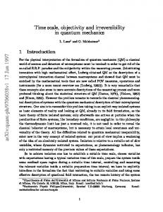
Caption Fig.1: The reservoirs occupy finite regions outside C0 , e.g. sectors Ca ⊂ R3 , a = 1, 2 . . .. Their particles are constrained to have a total kinetic energy Ka constant, by suitable forces ϑa , so that the reservoirs “temperatures” Ta , see Eq.(2), are well defined. Forces and potentials will be supposed smooth, i.e. analytic, in their variables aside from impulsive elastic forces describing shocks, allowed here to model shocks with the containers walls and possible shocks between hard core particles. In conclusion the equations of motion of the system in its phase space F , [6], def

F = (C0N0 × R3N0 ) ×

Y

(CaNa × Ba ) ≡ F0 ×

Y

Fa (4)

a

a≥1 1

where Ba is the sphere or radius (3Na kB Ta ) 2 in velocity space R3Na , can be written as ¨ 0,j = −∂X0,j W + Fj , X ¨ a,j = −∂Xa,j W − ϑa,j , X

j = 1, . . . , N0 j = 1, . . . , Na

(5)

with ϑa given by Eq.(3) and F the external ¿ forces in˙ X) the configutroduced after Eq.(1). Denoting St (X, def ˙ X) = (X ˙ a , Xa )a=0,...,n ration into which initial data (X, evolve in time t, a further condition has to be added that expresses the physical property that thermostats are ef˙ X), except ficient. Namely for all initial data x = (X, possibly for a set of data x of zero volume in F , the limit 1 T →∞ T lim

Z

0

T

˙ X)) dt = f (St (X,

Z

f (y)µ(dy)

(6)

F

exists for all smooth functions f and is independent of ˙ X), thus defining a probability distribution µ on F . (X,

This of course puts restrictions on the kind of forces acting on particles: it has to be stressed that the condition that thermostat forces be “efficient” enough (impeding, for instance, an indefinite build up of the energy) is strong but it has to be assumed. It imposes on the potentials conditions that are not well understood, although they seem empirically (i.e. in simulations) verified with the simplest choices of molecular potentials, [7]. The notion of thermostat just described has evolved in the last decades and, while it will continue to evolve, it seems to me that it has already reached a point in which one can lay down the above precise notion on which to base a few general considerations, [6]. The class of thermostats just considered is general enough for our purposes and is amply used in numerical simulations. The probability distribution µ in Eq. (6) is called the SRB distribution or SRB statistics. Typically one is interested in studying time averages of observables depend˙ 0 , X0 ) and not on ing only on the system coordinates (X the thermostats coordinates: in such case one needs only to know the distribution µC0 obtained by restricting the distribution µ to such observables: also µC0 will be naturally called the SRB distribution for the system. Remarks: (1) The time evolution maps St , acting on the full phase space F , will have the group property St · St′ = St+t′ and the SRB distribution µ will be invariant under time evolution. The SRB distribution µ is said to describe, and is identified with, a stationary state of the system; it depends on the parameters on which the forces acting on the system depend, e.g. |C0 | (volume) and more generally Φ (strength of the forcings), on the parameters that characterize the thermostats like their def phase space surfaces Fa , i.e. βa = (kB Ta )−1 , etc. The collection of SRB distributions obtained by letting the parameters vary defines a nonequilibrium ensemble. (2) Finite thermostats are an idealization of the apparently more appealing infinite thermostats in which the particles have a density ρa and an empirical distribution which asymptotically (at infinity) is Gibbsian with temperatures Ta , [6]: and in such infinite thermostats the temperature should stay necessarily constant because the local interaction between the particles in C0 and those in the thermostats cannot alter the velocity distribution of the thermostat particles at large distance, at least not if the thermostats act as physically expected. (3) One could imagine replacing the forces, Eq. (3), that keep the temperature constant, with other thermostats with which the particles in the containers Ca are in turn in contact: this is a matter of where we decide to stop in our investigation of the properties of what we call “system”. Should we be interested in what really happens in the containers Ca we would have to add them to what we call “system” and model their interactions with other thermostats. In this respect the Gaussian forces that act on the particles in the containers Ca are a model of further thermostats that act on the particles in Ca . If one

3 wants to avoid completely the forces (Gaussian as in Eq. (3) or of some other form) that fix the temperatures of the thermostats then one would be forced to consider infinitely extended Ca ’s. But unless the infinitely extended systems consist of non interacting particles, an important exception, see [8], not only this would lead to several conceptual problems (like existence of solutions to the equations of motion, phase transitions in the thermostats, nature of the statistical properties of the motions inside the thermostats) but it would also be possibly not needed, as in the end we are interested only in the statistical properties of the motions in the region C0 , i.e. on the finite system we started with. In fact the idea of using finite thermostats to study nonequilibrium statistical mechanics, [5], has been the source of the progress in the field in the last decades. Remark: Besides the mentioned relation with the “exactly soluble” case of [8], the above setting is very close to [1] which considers what has become known as transient properties of the fluctuations (see also [9]): and attempts to found on them a study of stationary states of systems like the ones considered here. The (CH) in this reference is present in the form of assumptions on the correlation functions on the stationary states of the system and thermostats. The latter works focus on thermostats which keep their temperature constant because they are infinite (sub)systems rather than finite isokinetic (sub)systems. The finite thermostats, considered here, allow us to look at the problem from a different viewpoint. It becomes possible to define entropy creation rate, to identify it with a contribution to the phase space contraction and to study the mechanism behind the irrelevance of the variations of the very large amount of energy stored in the reservoirs for what concerns the analysis of the large fluctuation relations. In the approach of the present paper the condition of strict positivity of the average phase space contraction plays a key role and the restrictions on the size of the fluctuations which satisfy the (FT) also appears in the results; and the theory of the larger fluctuations (and their exponential tails) could be borrowed from [10]. 2. Processes A process, denoted Γ, transforming an initial stationary state µini ≡ µ0 under forcing Φini ≡ Φ0 into a final stationary state µf in ≡ µ∞ under forcing Φf in ≡ Φ∞ will be defined by a piecewise smooth function t → Φ(t), t ∈ [0, +∞) , varying between Φ(0) = Φ0 to Φ(+∞) = Φ∞ . For intermediate times 0 < t < ∞ the time evolution ˙ X) → x(t) = S0,t x is generated by the equations x = (X, Eq. (5) with initial state in F and Φ(t) replacing Φ: it is a non autonomous equation. The time dependence of Φ(t) could for instance be due to a motion of the container walls which changes the vol˙ X) evolve at ume Vt = |C0 |: hence the points x = (X, time t in a space F (t) which also may depend on t. However here no time dependence of the thermostats temperature will be considered. It could be introduced as in

[1] by imagining that the potential coupling the system and the thermostats is time dependent so that interaction with each termostat could be switched on or off at will: such extra freedom and generality might require extensions of what is done here. During the process the initial state evolves into a state µt attributing to an observable Ft (x) defined on F (t) an average value given by hFt i =

Z

F (t)

def

µt (dx)Ft (x) =

Z

µ0 (dx)Ft (S0,t x) (7)

F (0)

We shall also consider the probability distribution µSRB,t which is defined as the SRB distribution of the dynamical system obtained by “freezing”Vt , Φ(t) at the value that they take at time t and imagining the time to further evolve until the stationary state µSRB,t is reached: in general µt 6= µSRB,t . Of course the existence of µSRB,t has to be assumed a priori and this can be implied by the general Chaotic Hypothesis, [11]: which states that Motions of a chaotic system, developing on its attracting set, can be assumed to follow an evolution with the properties of an Anosov system. This means that in the physical problems just posed, Eq. (5) with F, ϑ time independent, the motions are so chaotic that the attracting sets on which their long time motion takes place can be regarded as smooth surfaces on which motion is highly unstable. More precisely (i) around every point of F three planes Ms (x), Mu (x), Mm (x) can be identified which vary continuously with x, which are covariant (i.e. the planes at a point x are are mapped, by the evolution flow St , into the corresponding planes around St x) and (ii) the planes, called stable, unstable and marginal, with respective positive dimensions ds > 0, du > 0 and dm = 1 adding up to the dimension of F , have the property that infinitesimal lengths on the stable plane and on the unstable plane of any point contract at exponential rate as time proceeds towards the future or towards the past, respectively. The length along the marginal direction neither contracts nor expands (i.e. it varies relative to the initial value staying bounded away from 0 and ∞): its tangent vector is parallel to the velocity in phase space. In cases in which time evolution is discrete, and determined by a map S, the marginal direction is missing. (iii) over a time t, positive for the stable plane and negative for the unstable plane, the lengths contraction is exponential, i.e. lengths contract by a factor uniformly bounded by Ce−κ|t| with C, κ > 0. (iv) there is a dense trajectory. The Ergodic Hypothesis provides us with an expression for the equilibrium averages (as integrals over the normalized Liouville distribution on the energy surface): likewise the Chaotic Hypothesis provides us with the existence and a formal expression for the averages (i.e. for the SRB distribution), [12].

4 Of course the hypothesis is only a “beginning” and one has to learn how to extract information from it, as it was the case with the Liouville distribution once the Ergodic Hypothesis guaranteed it as an appropriate distribution for the study of the statistics of motions in equilibrium, [10]. 3. Heat generation The work La in Eq. (3) will be interpreted as heat Q˙ a ceded, per unit time, by the particles in C0 to the ath thermostat (because the “temperature” of Ca remains constant). The entropy creation rate due to heat exchanges between the system and the thermostats can, therefore, be naturally defined as

˙ X) def σ 0 (X, =

Na X Q˙ a k T a=1 B a

(8)

Remarks: (1) It is natural to define Eq. (8) as “heatexchanges entropy creation” rate because it is the amount of work per unit time that the system performs on the thermostats which nevertheless keep their temperature (identified with the kinetic energy) constant. (2) The above definition of “heat exchanges entropy creation” does not require any definition of entropy itself for the system: it only requires the notion of entropy variation of a reservoir considered as a system able to absorb work without changing it into mechanical work nor into its temperature variations. The latter is the “classical” definition of entropy variation of a reservoir. (3) If the thermostats temperatures are equal, i.e. Ka ∼ 3 −1 and Φ = 0, or Φ is conservative so that its 2 Na β potential can be imagined merged in U0 , it is possible to check that the SRB distribution, if existing, is necessarily −1 −β(K0 +U0 +

P

µSRB (dx) = Z Q e · a>0 δ(Ka −

a>0

Ua +

3Na −1 2β )

P

a>0

Wa )

· dV dX

· (9)

where dx = dV dX = phase space volume element, Ka are the kinetic energies of the various subsystems, a = 0, 1, . . . and Z is a normalization factor. Hence this is a Gibbs distribution in one of the equivalent, if unusual, equilibrium ensembles at temperature (kB β)−1 and denNa , a = 0, . . . , n. This is an important sities ρa = |C a| consistency check, following (and extending) [5]. 4, Irreversibility degree It is one of the basic tenets in Thermodynamics that all (nontrivial) processes between equilibrium states are “irreversible”: only idealized (strictly speaking nonexistent) “quasi static” processes can be reversible. The question that is addressed in the following is whether irreversibility can be made a quantitative notion at least in models based on microscopic evolution, Eq. (5). ¨ = Ξ(X, ˙ Write Eq. (5) as X P X) = Ξ(x) with x = (x1 , . . . , x˙ 1 , . . . , x˙ 3Ntot ), Ntot = a Na . Given a process Γ let

def

σtΓ (x) = − divergence(x) ≡ −

3N tot X

∂x˙ i Ξi (x)

(10)

i=1

which has the meaning of rate at which the phase volume around x contracts because of the forces action. Phase space volume can also change because new regions become accessible (or inaccessible) so that the total phase space contraction rate, denoted σtot,t , in general will be different from σtΓ . It is reasonable to suppose, and in some cases it can even be proved (e.g. in the example considered in remark (3) of Sect.5), that at every time t the configuration S0,t x is a “typical” configuration of the “frozen” system if the initial x was typical for the initial distribution µ0 : i.e. it Q will be a point in F (t) = VtN ×RN × Fa whose statistics under forces imagined frozen at their values at time t will be µSRB,t , see comments following Eq.(7). Since we consider as accessible the phase space occupied by the attractor of a typical phase space point, the volume variation contributes an extra σtv (x) to the phase space variation via the rate at which the volume |Ft | contracts, namely σtv (x) = −

1 d |Ft | V˙ t = −N |Ft | dt Vt

(11)

which does not depend on x as it is a property of the phase space available to (any typical) x. A calculation of the divergence −σ Γ of Eq. (5), see also Eq. (3), shows that (keeping properly into account that the momentum part of phase space is a sphere) ˙ X) = P σ Γ (X,

a>0

˙ a −U˙ a 3Na −1 Q 3Na kB Ta

≃

P

a>0

˙a Q kB Ta

− U˙

(12)

def P (3Na −1) Ua −1 if U = a 3Na kB Ta ; in the last step O(Na ) has been neglected (for simplicity and for consistence with macroscopic thermodynamics where Na are extremely large: it would not be difficult to keep track of it, however). Therefore the total phase space contraction per unit time can be expressed as, see Eq. (3),Eq. (8),

˙ X) = σtot (X,

X Q˙ a V˙ t −N − U˙ kB Ta Vt a

(13)

i.e. there is a simple and direct relation between phase space contraction and entropy creation rate, [6]. Eq. (12) shows that their difference is a “total time derivative”. In studying stationary states N V˙ t /Vt = 0, and the interpretation of U˙ is of “reversible” heat exchange between system and thermostats. In this case, in some respects, the difference U˙ can be ignored. For instance in the study of the fluctuations of the average over time of entropy creation rate in a stationary state the term U˙ gives no contribution, or it affects only the very large fluctuations, [10, 13] if the containers Ca are very large (or

5 if the forces between their particles can be unbounded, which we are excluding here for simplicity, [10]). Even in the case of processes the quantity U˙ has to oscillate in time with 0 average on any interval of time (t, ∞) if the system starts and ends in a stationary state. For the above reasons we define the entropy creation rate in a process to be Eq. (13) without the U˙ term: ˙ X) = ε(X,

X Q˙ a V˙ t −N kB Ta Vt a

(14)

It is interesting, and necessary, to remark that in a stationary state the time averages of ε, denoted ε+ , and of P Q˙ a+ P Q˙ a ˙ a kB Ta , coincide because N Vt /Vt = a kB Ta , denoted 0, as Vt = const, and U˙ has zero time average being a total derivative. On the other hand under very general assumptions, much weaker than the Chaotic Hypothesis, the time average of the phase space contraction rate is ≥ 0, [14, 15], so that in a stationary state: X Q˙ a+ ε+ ≡ ≥0 (15) kB Ta a which is a consistency property that has to be required for any proposal of definition of entropy creation rate. Remarks: (1) In stationary states the above models are a realization of Carnot machines: the machine being the system in C0 on which external forces F work leaving the system in the same stationary state (a special “cycle”) but achieving a transfer of heat between the various thermostats (in agreement with the second law, see Eq. (8),Eq. (15), only if ε+ ≥ 0). P Q˙ a ˙ (2) In a stationary state σtot = a kB Ta − U will satisfy, under the Chaotic Hypothesis of Sec.2, a fluctuation relation, see [11, 16], since the dynamics Eq. (5) is time reversible: the large fluctuations of the quantity RT P ˙a Q ˙ p = ε1+ T1 0 ( a>0 kB Ta + U) dt will be controlled by a rate function ζ(p) satisfying ζ(−p) = ζ(p) − pε+ , see [10, 16]. However the term U˙ will not contribute to the relation because U is bounded, [10]. Therefore the flucRT P ˙a Q tuations of p = ε1+ T1 0 a>0 kB Ta dt will have exactly the same rate function. (3) Note,P however, that U can be very large (being of the order of a>0 Na ) if the thermostats are large and its contribution P to the averages of σtot tends to 0 as slowly as T −1 O( a>0 Na ). Hence the time necessary to see the fluctuation relation satisfied with prefixed accuracy when p is defined as the average of σtot may be enormously larger than the time necessary to see the fluctuation relation satisfied with p defined as the average of P Q˙ a a kB Ta . In the case of infinite reservoirs, considered in [1], this leads to an “apparent” violation of the (FT) as pointed out in [13] quantitatively in a special case and extended in [10] (see the “exponential tails in the latter references). (4) Therefore the Fluctuation Theorem holds for the

P Q˙ a physically interesting a kB Ta as a consequence of its validity for σtot and it becomes visible over much shorter time scale, independent on the size of the thermostats. (5) The above derivation of the (FT) is somewhat unsatisfactory because one cannot turn it into a mathematically complete theorem even if one is willing to make strong assumptions (like the assumption that the system is “Anosov” in absence of external forces and of thermostats): this is because the lack of a boundedness constraint imposed on the kinetic energy in C0 makes phase space unbounded; more physically it is the above “efficiency” assumption on the interaction between thermostats and system which is not properly understood mathematically but which is necessary in the proof. In this respect the results here suffer from some of the drawbacks in the analysis in [1] (see comments after eq. (33) and at the end of Sec. 4 of the latter reference) which also relies on an efficiency assumption on the thermostats. Adding a constraint that the total kinetic energy of the system in C0 (as done in [17]) would trivially solve this problem but it would be physically quite unsatisfactory. Coming back to the question of defining an irreversibility degree of a process Γ we distinguish between the (non stationary) state µt into which the initial state µ0 evolves in time t, under varying forces and volume, and the state µSRB,t obtained by “freezing” forces and volume at time t and letting the system settle to become stationary, see coments following Eq. (7). We call εt the entropy creation rate Eq. (14) and εsrb the entropy creation rate in t the “frozen” state µSRB,t . The proposal is to define irreversibility degree I(Γ) or irreversibility time scale I(Γ)−1 of a process Γ by setting: Z ∞ 2 1 I(Γ) = 2 hεt iµt − hεsrb i dt (16) t SRB,t N 0 If the Chaotic Hypothesis is assumed then the state µt will evolve exponentially fast under the “frozen evolution” to µSRB,t . Therefore the integral in Eq. (16) will converge for reasonable t dependences of Φ, V . A physical definition of “quasi static” transformation is a transformation that is “very slow”. This can be translated mathematically into an evolution in which Φt evolves like, if not exactly, as Φt = Φ0 + (1 − e−γt )(Φ∞ − Φ0 ).

(17)

An evolution Γ close to quasi static, but simpler for computing I(Γ), would proceed changing Φ0 into Φ∞ = Φ0 +∆ by ∆/δ steps of size δ, each of which has a time duration tδ long enough so that, at the k-th step, the evolving system settles onto its stationary state at field Φ0 +kδ. If the corresponding time scale can be taken = κ−1 , independent of the value of the field so that tδ can be defined by δe−κtδ ≪ 1, then I(Γ) = const δ −1 δ 2 log δ −1 because the variation of σ(k+1)δ,+ − σkδ,+ is, in general, of order δ as a consequence of the differentiability of the SRB states with respect to the parameters, [18].

6 5, Comments and examples Remarks: (1) A drawback of the definition proposed in Sec.4 is that although hεsrb t iSRB,t is independent on the metric that is used to measure volumes in phase space the quantity hεt iµt depends on it. Hence the irreversibility degree considered here reflects also properties of our ability or method to measure (or to imagine to measure) distances in phase space. One can keep in mind that a metric independent definition can be simply obtained by minimizing over all possible choices of the metric: but the above simpler definition seems, nevertheless, preferable. (2) It is I(Γ) ≥ 0, but I have not been able to prove (except in the limit of a quasi static process) that I(Γ) > 0: this is a natural question to raise. (3) Suppose that a process takes place because of the variation of an acting conservative force, for instance because a gravitational force changes as a large mass is brought close to the system, while no change in volume occurs and the thermostats have all the same temperature. Then the ”frozen” SRB distribution, for all t, is given by Eq. (9) and hεsrb iSRB,t = 0 (because the ”frozen equations” admit a SRB distribution which has a density, see Eq. (9), in phase space). The isothermal process thus defined has therefore I(Γ) > 0 except, possibly, if it is isentropic, i.e. if initial and final thermodynamic entropies are equal. In fact the latter are cases in which the initial, intermediate and final states are described by a density function ρt (x) on phase space hence, [14], it is hεsrb t iSRB,t = 0 and,[19], R d hεt iµt = − dt ρt (x) log ρt (x) dx. Since the initial and final states are equilibrium states this means that if the initial and final thermodynamic entropies (i.e. Gibbs’) are different it must be hεt iµt 6= 0 on a set of times of positive measure and I(Γ) > 0 and we expect it to be of order δ (see last comment in Sect.4). On the other hand if the thermodynamic entropies are the same and Γ is almost quasi static then the discussion at the end of Sec.4 shows that the irreversibility time scale may tend to +∞ when δ → 0 much faster than in the cases in which the entropies differ (e.g. as δ 3 rather than as δ). (4) The comment (3) shows that if a connection between thermodynamic entropy and irreversibility scale can be established at all it will neither be too direct nor too simple because in the considered isothermal process linking two equilibrium states there is, in general, a non zero entropy variation hence I(Γ) > 0 but, if performed very slowly, it can be close to be reversible both in the classical Thermodynamics and in the irreversibility scale senses. (5) Consider a typical irreversible process. Imagine a gas in an adiabatic cylinder covered by an adiabatic piston and imagine to move the piston. The simplest situation arises if gravity is neglected and the piston is suddenly moved at speed w. Unlike the cases considered so far, the absence of thermostats (adiabaticity of the cylinder) imposes an extension of the analysis. In this case the phase space is the

surface of constant energy in C0N0 × R3N0 rather than the full C0N0 × R3N0 . Therefore if the piston moves at a speed which is too slow (i.e. slower than the maximum velocity of the particles on the energy surface) it will change the total energy of the gas in a way that depends on the special configuration initially chosen. Therefore the simplest situation arises when the piston is moved at speed so large that no energy is gained or lost by the particles because of the collisions with the moving wall (this is, in fact, a ¿ case in which there are no such collisions). This is an extreme idealization of the classic Joule-Thomson experiment. Let S be the section of the cylinder and Ht = H0 + w t be the distance between the moving lid and the opposite base. Let Ω = S Ht be the cylinder volume. In this case the volume of phase space changes only because the boundary moves and it increases by N w S ΩN −1 per unit time, i.e. its rate of increase is N Hwt . L Hence hεt it is −N Hwt , while εsrb is the ≡ 0. If T = w t duration of the transformation (”Joule-Thomson” process) increasing the cylinder length by L, then RT
2 I(Γ) = N −2 0 N 2 Hwt dt −T−→∞ −−→ w H0 (HL0 +L) (18) and the transformation is irreversible. The irreversibility time scale approaches 0 as w → ∞, as possibly expected. If H0 = L, i.e. if the volume of the container is doubled, w then I(Γ) = 2L and the irreversibility time scale of the process coincides with its ”duration”. (6) A different situations arises if in the context of (5) the piston is replaced by a sliding lid which divides the cylinder in two halves of height L each: one empty at time zero and the other containing the gas in equilibrium. At time 0 the lid is lifted and a process Γ′ takes place. In this case V˙ t = V δ(t) because the volume V = S L becomes suddenly double. Therefore the evaluation of the irreversibility scale yields ′

I(Γ ) = N

−2

Z

∞

N 2 δ(t)2 dt ≡ +∞

(19)

0

so that the irreversibility becomes immediately manifest, I(Γ′ ) = +∞, I(Γ′ )−1 = 0. This idealized experiment is rather close to the actual Joule-Thomson experiment. In the latter example it is customary to estimate the degree of irreversibility at the lift of the lid by the thermodynamic equilibrium entropy variation between initial and final states. It would of course be interesting to have a general definition of entropy of a non stationary state (like the states µt at times (t ∈ (0, ∞) in the example just discussed) that would allow connecting the degree of irreversibility to the thermodynamic entropy variation in processes leading from an initial equilibrium state to a final equilibrium state, see [20]. The time scale introduced in Eq.(16) refers to the entire process rather than to what happens to the system only; it might have alternative interpretations: but it seems a quantity of interest in itself.

7 Acknowledgements: I am indebted to F. Bonetto, A. Giuliani and F. Zamponi for many ideas, discussions and for earlier collaborations that preceded and stimulated the de-

[1] [2] [3] [4] [5] [6] [7] [8] [9] [10] [11]

C. Jarzynski, Journal of Statistical Physics 98, 77 (1999). G. Gallavotti, Physica D 112, 250 (1998). G. Gallavotti, cond-mat/0402676 (2004). D. Ruelle, Journal of Statistical Physics 95, 393 (1999). D. Evans and G. Morriss, Statistical Mechanics of Nonequilibrium Fluids (Academic Press, New-York, 1990). G. Gallavotti, cond-mat/0510027 (2005). G.Gallavotti, Open Systems and Information Dynamics 6, 101 (1999). J.P.Eckmann, C. Pillet, and L. R. Bellet, Communications in Mathematical Physics 201, 657 (1999). G. Gallavotti and E. Cohen, Physical Review E 69, 035104 (+4) (2004). F. Bonetto, G. Gallavotti, A. Giuliani, and F. Zamponi, cond-mat/0507672 (2005). G. Gallavotti and E. Cohen, Physical Review Letters 74, 2694 (1995).

velopment of this work and to a referee for pointing out the reference to Jarzynski’s paper, [1].

[12] G. Gallavotti, F. Bonetto, and G. Gentile, Aspects of the ergodic, qualitative and statistical theory of motion (Springer Verlag, Berlin, 2004). [13] R. V. Zon and E. Cohen, Physical Review Letters 91, 110601 (+4) (2003). [14] D. Ruelle, Journal of Statistical Physics 85, 1 (1996). [15] D. Ruelle, Communications in Mathematical Physics 189, 365 (1997). [16] G. Gallavotti, Mathematical Physics Electronic Journal (MPEJ) 1, 1 (1995). [17] G. Gallavotti, Physical Review Letters 77, 4334 (1996). [18] D. Ruelle, Communications in Mathematical Physics 187, 227 (1997). [19] L. Andrej, Physics Letters 111A, 45 (1982). [20] S. Goldstein and J. Lebowitz, Physica D 193, 53 (2004).

REVTEX