Koichi Yamazaki, Hans L. Bodlaender, Babette de Fluiter, Dimitrios M. Thilikos. Department of Computer Science, Utrecht University,. P.O. Box 80.089, 3508 TB ...
Isomorphism for Graphs of Bounded Distance Width� Koichi Yamazaki, Hans L. Bodlaender, Babette de Fluiter, Dimitrios M. Thilikos Department of Computer Science, Utrecht University, P.O. Box 80.089, 3508 TB Utrecht, the Netherlands E-mail: f g koichi,hansb,babette,sedthilk @cs.ruu.nl
Abstract
In this paper, we study the Graph Isomorphism problem on graphs of bounded treewidth, bounded degree or bounded bandwidth. Graph Isomorphism can be solved in polynomial time for graphs of bounded treewidth, pathwidth, or bandwidth, but the exponent depends on the treewidth, pathwidth, or bandwidth. Thus, we look for special cases where ` xed parameter tractable' polynomial time algorithms can be established. We introduce some new and natural graph parameters: the (rooted) path distance width, which is a restriction of bandwidth, and the (rooted) tree distance width, which is a restriction of treewidth. We give algorithms that solve Graph Isomorphism in O(n2 ) time for graphs with bounded rooted path distance width, and in O(n3 ) time for graphs with bounded rooted tree distance width. Additionally, we show that computing the path distance width of a graph is NP-hard, but both path and tree distance width can be computed in O(nk+1 ) time, when they are bounded by a constant k; the rooted path or tree distance width can be computed in O(ne) time. Finally, we study the relationships between the newly introduced parameters and other existing graph parameters.
1 Introduction In this paper, we consider the Graph Isomorphism problem, for graphs for which certain parameters can be assumed to be small constants. We are especially interested in Graph Isomorphism on graphs where either the treewidth, bandwidth, or degree of the graph is bounded, as there are many interesting graph classes which have a bound on one of these parameters (see e.g. [2]). For these parameters, it has been shown that when the parameter is a constant, then Graph Isomorphism is polynomial time solvable (see [12] for bounded degree, and [3] for bounded treewidth and bandwidth). However, in each of these three cases, the exponent of the algorithm grows with the parameter. Thus, a question is, whether algorithms exist for Graph Isomorphism with a running time � The rst author was supported by Ministry of Education, Science, Sports and Culture of Japan as Oversea's Research Scholar. The second and last author were partially supported by ESPRIT Long Term Research Project 20244 (project ALCOM IT: Algorithms and Complexity in Information Technology). The third author was supported by the Foundation for Computer Science (S.I.O.N) of the Netherlands Organisation for Scienti c Research (N.W.O.). The last author was supported by the Training and Mobility of Researchers (TMR) Program, (EU contract no ERBFMBICT950198).
1
O(f (k)nc), c a small constant, k the maximum degree / treewidth / bandwidth / . . . / of the graph; in other words, whether Graph Isomorphism is xed parameter tractable (in the sense of the xed parameter complexity theory of Downey and Fellows, see e.g. [8, 9]), with the maximum degree / treewidth / bandwidth / . . . / as parameter. Thus, we are looking for answers to the questions whether Graph Isomorphism is xed parameter tractable for the case that the parameter is the degree, treewidth or bandwidth of the graph. These questions are apparently hard. In this paper, we are able to solve some interesting special cases of these problems. For this, several natural graph parameters are introduced: the (rooted) path distance width, and the (rooted) tree distance width. The notion of path distance width can be seen to have a close relation to bandwidth; the notion of tree distance width is a natural tree-like generalisation of this notion, with a close relationship to treewidth. This paper is organised as follows. In section 2 we prove that the rooted path (tree) distance width of a graph can be computed in O(ne) time, that computing the path distance width of a graph is NP-hard, but if the path or tree distance width is at most some xed constant k, then the minimum path (tree) distance width can be computed in O(nk+1 ) time. The main results of the paper can be found in Section 3: it is shown that Graph Isomorphism is solvable in O(n2 ) time for graphs with bounded rooted path distance width, thus solving a signi cant special case of Graph Isomorphism for graphs of bounded bandwidth. Furthermore, it is shown that Graph Isomorphism is solvable in O(n3 ) time for graphs with bounded rooted tree distance width, which solves a special case for Graph Isomorphism for graphs of bounded treewidth. In Section 4, the relations between the di�erent considered parameters are investigated.
2 De nitions and Complexity Results for Distance Width The graphs we consider are simple, undirected and connected, and contain no self loops. For a graph G, we denote its set of vertices by V (G) and its set of edges by E (G). Also, we denote as G[S ] the subgraph of G induced by S � V (G). For two graphs G and H , a function f : V (G) ! V (H ) is called an isomorphism (from G to H ) if f is a bijection and for each v; w 2 V (G), fv; wg 2 E (G) i� ff (v); f (w)g 2 E (H ). Two graphs G and H are isomorphic if there is an isomorphism from G to H . The Graph Isomorphism problem is the problem of checking for two given graphs whether they are isomorphic. A graph parameter is a function which maps each graph to a positive integer. We rst review a number of graph parameters. � A tree decomposition of a graph G = (V; E ) is a pair (fXi j i 2 I g; T = (I; F )), where fXi j i 2 I g is a collection of subsets of V and T is a tree, such that { S Xi = V (G), i2I
{ for each edge fv; wg 2 E , there is an i 2 I such that v; w 2 Xi , and { for each v 2 V the set of nodes fi j v 2 Xi g forms a subtree of T. The width of a tree decomposition (fXi j i 2 I g; T = (I; F )) equals max (jXi j , 1). i2I
The treewidth of a graph G is the minimum width over all tree decompositions 2
of G. The corresponding graph parameter (which is the function that maps each graph to its treewidth) is denoted by T W . A (linear) layout of a graph G is a one-to-one function f : V (G) ! f1; : : : ; jV (G)jg.
� The bandwidth of a layout f of a graph G is de ned as fu;vmax jf (u) , f (v)j. g2E (G)
The bandwidth of a graph G is the minimum bandwidth over all layouts of G. The corresponding graph parameter is denoted by BW .
For a given graph G and two vertices u; v 2 V (G), dG (u; v) denotes the distance between u and v, which is the number of edges on a shortest path between u and v. For a set S � V (G) and a vertex w 2 V (G), dG (S; w) denotes min d (v; w). v2S G
� A tree distance decomposition of a graph G = (V; E ) is a triple (fXi j i 2 I g; T = (I; F ); r), where { S Xi = V (G) and for all i 6= j , Xi \ Xj = ;, i2I
{ for each v 2 V , if v 2 Xi, then dG(Xr ; v) = dT (r; i), and { for each edge fv; wg 2 E , there are i; j 2 I such that v 2 Xi, w 2 Xj and either i = j or fi; j g 2 F . Node r is called the root of the tree T , and Xr is called the root set of the tree distance decomposition. The width of a tree distance decomposition (fXi j i 2 I g; T; r) is equal to max jX j. The tree distance width of a graph G is the minimum i2I i width over all possible tree distance decompositions of G. The corresponding graph parameter is denoted by T DW . � A rooted tree distance decomposition of a graph G = (V; E ) is a tree distance decomposition (fXi j i 2 I g; T = (I; F ); r) of G in which jXr j = 1. The rooted tree distance width of a graph G is the minimum width over all rooted tree distance decompositions. The corresponding graph parameter is denoted by RT DW . � The (rooted) path distance decomposition and the parameter of (rooted) path distance width of a graph G = (V; E ) are de ned similar to the (rooted) tree distance decomposition and (rooted) tree distance width, but now the tree T is required to be a path. For reasons of simplicity we will denote a (rooted) path distance decomposition as (X1 ; X2 ; : : : ; Xt ), where X1 is the root set of the decomposition. We denote the corresponding graph parameters by PDW , and RPDW , respectively. It is easy to check that for any graph G, T W (G) � 2T DW (G) , 1, T DW (G) � RT DW (G), BW (G) � 2PDW (G) , 1 and PDW (G) � RPDW (G). Hence xed parameter tractability of Graph Isomorphism for T W implies the same for T DW and RT DW , and xed parameter tractability of Graph Isomorphism for BW implies the same for PDW and RPDW . Also, showing that for Graph Isomorphism is xed parameter tractable for e.g. RPDW might give more insight in whether it is xed parameter tractable for BW . Therefore, we study the complexity of Graph Isomorphism on graphs for which PDW , RPDW , T DW or RT DW is bounded. 3
Procedure GET-TDD
input: a graph G = (V; E ) and a root set S output: the minimal tree distance decomposition (fXi j i 2 I g; T = (I; F ); r), (Xr = S ) 1: for any v 2 V set distance(v) = dG (S; v); 2: m := max distance(v); v2V 3: I := ;; F := ;, and h := 0; 4: for any i; 0 � i � m + 1 set Vi = fv 2 V j distance(v) = ig; 5: for i := m down to 0 do 6: Compute the connected components of G[fv 2 V j i � distance(v) � i + 1g]; /* We call the connected components S1 ; : : : ; St */ 7: for j := 1 to t do 8: Xh+j := Sj , Vi+1 ; 9: Add edges fv; ug; v; u 2 Xh+j to E (G) such that G[Xh+j ] becomes connected; 10: I := I [ fh + j g; 11: F := F [ ffh + j; kg j Xk � Sj ^ k � hg; 12: od 13: h := h + t; 14: od 15: end.
Figure 1: Procedure GET-TDD(G; S ). For a given graph G and S � V (G), there is a unique path distance decomposition of G with root set S , and this decomposition can be found in O(e) time (e = jE (G)j): for each vertex v 2 V (G), compute dG (S; v) using breadth rst search. Then for each possible distance d, make a node Xd containing all vertices with distance d to S . De nition Let D = (fXi j i 2 I g; T = (I; F ); r) be a tree distance decomposition of G. Given a vertex v 2 I we denote as Tv the connected subtree of T induced by all the nodes in I that are connected with r via paths containing v. Finally, given a node i 2 I we set V (D; i) = S Xw . w2V (Ti )
For a given graph G and set S � V (G), there may be more than one tree distance decomposition with root set S . However we de ne the minimal tree distance decomposition of a graph G with root set S as follows. De nition Let D = (fXi j i 2 I g; T = (I; F ); r) be a tree distance decomposition of G. We call D minimal if, for each i 2 I , G[V (D; i)] is connected. An immediate consequence of the de nition above is that given a graph G and a root set S the minimal tree distance decomposition is uniquely de ned. Also, it can be found with procedure GET-TDD presented in Figure 1, which can be made to run in O(e) time. Theorem 2.1 Given a graph G and a set S � V (G), we can compute in O(jE (G)j) time the unique path distance decomposition with root set S , or the unique minimal tree distance decomposition with root set S . 4
Proof. Let D = (fXi j i 2 I g; T = (I; F ); r) be some output of GET-TDD. It is easy to see that D is a tree distance decomposition of G. We will prove that for any i 2 I , G[V (D; i)] is connected. Let m = maxi2I dT (r; i). We will use induction on m , dT (r; i). If dT (r; i) = m, then it is clear from the algorithm that G[V (D; i)] is connected. Assume that for any i 2 I such that dT (r; i) > n (0 < n � m), G[V (D; i)] is connected. Let i 2 I such that dT (r; i) = n. Let also fi1 ; : : : ; it g � I be such that for all i� , 1 � � � t, dT (r; i� ) = n + 1 and ffi; i1 g; : : : ; fi; it gg � F . We will prove that G[V (D; i)] is connected, that is, we will show that for any pair of vertices v; u 2 V (D; i), there exists a path connecting u and v in G[V (D; i)]. From the induction hypothesis and the fact that all vertices in Ln+1 = Xi1 [ : : : [ Xit are adjacent to a vertex in Xi , we have that there exist two vertices v0 , u0 in Xi connected by some paths in G[V (D; i)] with v and u respectively. The connectivity of G[V (D; i)] follows now easily in the case where G[Xi [ Ln+1 ] is connected. Suppose that G[Xi [ Ln+1 ] is not connected. In this case we notice that Xi [ Ln+1 must induce one of the connected components computed during the (m , n + 1)th execution of step 5 (m is de ned at step 2). Clearly, each of these connected components became connected because of the addition of some number of edges connecting vertices in Xi� ; 1 � � � t during the (m , n)th execution of loop 7{12. We call these edges new edges and denote the current graph after the (n , 1)th loop by Gn . As there exists in Gn [Xi [ Ln+1 ] a path connecting v0 and u0 , such a path must contain a number of new edges (see Figure 2). From the induction hypothesis we have that any new edge corresponds to a path in G[V (D; i� )] connecting its endpoints for some �; 1 � � � t. Thus, we can construct a path in G[V (D; i)] connecting u0 and v0 . Therefore, there exists a walk (hence path) connecting u and v and the connectivity of G[V (D; i)] follows.
Xi
u’
v’
new edge
u’
v’
new edge
L n+1 X i1
X i2
X i3
u
X i4 v
u The graph after the 2nd execution of the loop defined by steps 6-13 in GET-TDD
The original graph
Figure 2: An example for the procedure GET-TDD. Step 1 uses breadth rst search to assign for each vertex in the graph its distance from the root set. This costs O(jE (G)j) time. Also loop 5{14 needs in total O(jE (G)j) time as the executions of step 6 use in total O(jE (G)j) time and each call of line 9 can be executed in O(jV (Xh+j )j) time. 2 5
v
From Theorem 2.1 and the fact that, if a graph has (rooted) tree or path distance width at most k, then e = O(kn), we get the following result.
Corollary 2.2 There is an algorithm that computes a rooted path (tree) distance decomposition of minimum width of a graph G in O(kn2 ) time, where k is the rooted path (tree) distance width of the graph. There is an algorithm that computes a path (tree) distance decomposition of minimum width of a graph in O(knk+1 ) time, where k denotes the path (tree) distance width of the graph. The following result concerns the complexity of (rooted) path (tree) distance width.
Theorem 2.3 The following problem is NP-complete even if the input graphs are trees.
Given a graph G and an integer k, does G have path distance width at most k?
Proof. The proof is based on a reduction from the following strongly NP-complete problem:
3Partition
A set A = fa1 ; : : : ; a3m g of positive integers and an integer value B such that B=4 < ai < B=2; 1 � i � 3m; m > 1, and P ai = mB . 1�i�3m Is there a partition of A into m disjoint sets A 1 ; A2 ; � � � ; Am such P that a = B; 1 � i � m?
Instance:
Question:
a2Ai
We describe a transformation that, given an instance of the 3Partition problem, outputs a tree T such that T has path distance width at most d i� the answer for the 3Partition problem is yes. Let c = 57m + 1 and d = c � B + 9m. T is constructed as follows: First we set Ui = fui;1; : : : ; ui;m g, Vi = fvi;1 ; : : : ; vi;cai g; 1 � i � 3m, and W = fw1 ; : : : ; w2d,12m g. Then, we de ne Ti = (fxg [ Ui [ Vi ; ffx; ui;1gg [ ffui;j ; ui;j +1 g jS1 � j � m , 1g [ ffvi;j ; ui;mg j 1 � j � c � aig); 1 � i � 3m. Now, set T = (W [ V (Ti ); ffx; wi g j
1 � i � 2d , 12mg [ ( S E (Ti ))) (see also Figure 3). 1�i�3m We will prove now that the 3Partition instance has a solution i� T has a path distance decomposition (X1 ; X2 ; : : : ; Xt ) with width at most d. Let fA1 ; A2 ; � � � ; Am g be a solution of the 3partition problem. We constructSa path distance decomposition as follows. We rst de ne f : f1; 2; : : : ; 3mg 7! fxg [ Ui 1�i�3m such that f (i) = x i� ai 2 A1 and f (i) = ui;j ,1 i� ai 2 Aj ; 2 � j � m. We set S = fw1; w2 ; � � � ; wd,3m g [ ff (1); : : : ; f (3m)g. Let (X1 = S; X2 ; : : : ; Xr ) be the path distance decomposition of G with root set S . Now we prove that for all i, 1 � i � r, jXi j � d. By the construction, we have that the cardinality of the root set S = X1 is no more than d. We also observe that XS2 contains d , 9m vertices from W , and at most 3m +2 � 3m vertices from UT = fxg[ Ui . So 1�i�3m jX2 j � d. It is now easy to see that for any i > 2; Xi must contain at most 3 � 3m vertices 1�i�3m
6
W c=57m+1 d=cB+9m
110101 00
w1
U
w2d-12m
x
u1,1
000101010 11 111 11 00 00 0 1 0 1 001010 11
u3m,1
1
u1,m
U
3m
ui,m
V1 V2 V3 V4 V5 V6 V7 V8
Vi
u3m,m V3m-2 V3m-1 V3m
3m ui,m
010101
vi,ca
vi,1
i
Vi
Figure 3: The reduction of Theorem 2.3. from UT and cai1 + cai2 + cai3 vertices from Vi1 [ Vi2 [ Vi3 where Aj = fai1 ; ai2 ; ail g is some set Aj of the solution of the 3Partition problem. Thus cai1 + cai2 + cai3 = cB and for any i > 2; Xi must contain at most d = cB + 9m vertices. Therefore, (X1 ; : : : ; Xr ) has distance width at most d. Suppose now that (X1 ; : : : ; Xt ) is a path distance decomposition of T that has width at most d. We prove that P there exists a partition of A = fa1 ; : : : ; a3m g into m disjoint sets A1 ; : : : ; Am such that a2Ai a = B; 1 � i � m. We distinguish two cases: Case 1: x 2 X1 . In this case we easily observe that W � X1 [ X2 and thus we have jX1 \ W j + jX2 \ W j = jW j = 2d , 12m. Using this and the fact that jX1 j; jX2 j � d, we have that 2d � jX1 j + jX2 j = jX1 , W j + jX1 \ W j + jX2 , W j + jX2 \ W j = jX1 , W j + jX2 , W j + 2d , 12m � jXi , W j + 2d , 12m ) jXi , W j � 12m; i = 1; 2. Let fRj j j � 1g be a collection of subsets of f1; 2; : : : ; 3mg such that i 2 Rj i� jXj \ Vij � cai , 12m. We rst claim that for all i, 1 � i � 3m, there exists at most one j � 1 such that i 2 Rj Suppose that for some i, there are j and j 0 such that j 6= j 0 ; i 2 Rj and i 2 Rj0 . In such a case we have that jXj \Vi j � cai ,12m and jXj 0 \Vi j � cai ,12m. As Xj \Xj 0 = ;, we conclude that jVi j � 2cai , 24m ) cai � 2cai , 24m ) 24m � cai � c = 57m + 1, a contradiction. We now claim that for all i, 1 � i � 3m, there exists a j � 1, such that i 2 Rj . 7
Choose j 0 such that ui;m 2 Xj 0 . Notice that for all v 2 Vi , either v 2 X1 or v 2 Xj 0 +1 . As X1 \ Vi � X1 , W , we have that jX1 \ Vi j � 12m and thus jXj 0 +1 \ Vi j � cai , 12m ) i 2 Rj0 +1 . We claim that if j = 1; 2 then Rj = ;. Indeed, suppose, on the contrary, that for some j = 1; 2 there exists an i; 1 � i � 3m such that i 2 Rj . In this case we have that jXj \ Vij � cai , 12m. But, as jXj , W j � 12m; j = 1; 2 and Xj \ Vi � Xj , W; j = 1; 2; 1 � i � 3m, we conclude that 12m � jXj , W j � jXj \ Vi j � cai , 12m � c , 12m = 57m + 1 , 12m = 45m + 1, a contradiction. Notice also that, as x 2 X1 , we have that V (T ) � X1 [ � � � [ Xm+2 and thus for all j � m + 3, Rj = ;. We now set Aj = fai j i 2 Rj +2 g; 1 � j � m. Clearly, A1 ; : : : ; Am is a partition of A. We claim that for all j , 1 � j � m,PjAj j � 3. Suppose, Pon the contrary that j � m, jAj j � 4. Then ai 2Aj jXj +2 \ Vi j � ai 2Aj (cai , 12m) � Pfor some(c Bj;+11 �, 12 m) � 4( cB4 + 4c , 12m) � cB + c , 48m � cB + 9m + 1 > d, a ai 2Aj 4 contradiction. From the claims above, we conclude that the sets A1 ; : : : ; Am form a partition of A into sets consisting of at most 3 elements. What now remains to be proven is that for all j , 1 � j � m, Pa2Aj a = B . Clearly, as P ai = mB , it is su�cient to prove that for all j , 1 � j � m, Pa2Aj a � B . For 1�i�3m this, we rst notice that c Pai 2Aj ai � Pai 2Aj (jXj +2 \ Vi j + 12m) � jXj +2 j + 36m � d + 36m = cBP+ 9m + 36m � cB + 45m. Finally, we have that Pai 2Aj ai � B + 45cm which implies ai 2Aj ai � B + b 45cm c = B (b 45cm c = 0 because c = 57m + 1 > 45m). Case 2: x 62 X1 . In this case we can easily see that X1 [ W 6= ; because otherwise, if x 2 Xi for some i, then W � Xi+1 , but jW j > d. So, x 2 X2 , and W � X1 [ X3 ) jX1 \ W j + jX3 \ W j = 2d , 12m. Using the fact that jX1 j; jX3 j � d and, using a similar argument as in Case 1, we have that jXi , W j � 12m, i = 1; 3. We de ne fRj j j � 1g as in Case 1 and following a similar argumentation, we deduce that any i 2 f1; : : : ; 3mg belongs to exactly one Aj . Also very similarly to Case 1 we have that if i = 1 or 3, then Rj = ;. Moreover, we claim that Rm+2 = ;. Suppose, on the contrary, that i 2 Rm+2 . This means that jXm+2 \ Vi j � cai , 12m and thus there exists some vertex w 2 Xm+2 that belongs in Vi . Notice now that, as dT (X1 ; w) = m + 1 � 3 we have that for all h, 1 � h � m, ui;h 2 Xh+1 and thus x 2 X1 , contradiction. (if x 2 Xi ; i > 2 then W � Xi+1 a contradiction) Finally, as x 2 X2 , and for all w 2 V (T ), dT (x; w) � m + 1, we easily conclude that for all j � m + 4, Xj = ; ) Rj = ;. We set A1 = fai j i 2 R2 g, Aj = faj j i 2 Rj +2g; 2 � j � m , 1 and Am = fai j i 2 Rm+3g. Following now the same steps as in Case 1, one can prove that A1; : : : ; Am is a partition of A into sets consisting of at most 3 elements such that for P all j , 1 � j � m, a2Aj a = B . 2
8
3 Graph Isomorphism for Graphs of Bounded Distance Width In this section, it is shown that the Graph Isomorphism problem is xed parameter tractable for graphs of bounded rooted path distance width or bounded rooted tree distance width. We present an algorithm with running time O(n2 ) that tests isomorphism for two graphs with rooted path distance width at most some constant k, and an algorithm with running time O(n3 ) that tests isomorphism for graphs with rooted tree distance width at most some constant k. Algorithm RPDW-ISO(G;H ) input: graphs G and H of rooted path distance width at most k. output: \Yes", if G is isomorphic to H ,
\No", otherwise. 1: Let DG = (X1G ; : : : ; XtGG ) be a rooted path distance decomposition of G with root set X1G = fvG g and rooted path distance width at most k. 2: for each vH 2 V (H ) do 3: let DH = (X1H ; : : : ; XtHH ) be a rooted path distance decomposition of G with root set X1H = fvH g; 4: if SUB-RPDW(DG; DH ) =true 5: then return \Yes"; 6: od 7: return \No"; 8 end
Procedure SUB-RPDW(DG ; DH ) input: decompositions DG = (X1G ; : : : ; XtGG ),
DH = (X1H ; : : : ; XtHH ),
output: \true", if DG is isomorphic to DH , \false", otherwise. 1: if tG 6= tH then return false 2: else let t tG ; 3: for i := 1 to t do 4: if jXiG j = jXiH j then return false; G 5: let Rt be the set of bijections from G[Xt ] to H [XtH ]; 6: if Rt = ; then return false; 7: for i := t , 1 downto 1 do 8: let Ri ! ;; 9: for each bijection f from G[XiG ] to H [XiH ] 10: if there existsG a bijection g 2 Ri+1 such that f [ g is an isomorphism from G[Xi [ XiG+1 ] to G[XiH [ XiH+1 ] 11: then Ri Ri [ ff g; 12: od 13: if R1 = 6 ; 14: then return true 15: else return false; 16: end.
De nition Let DG = (X1G ; : : : ; XtGG ) and DH = (X1H ; : : : ; XtHH ) be two path distance
decompositions of graphs G and H respectively. We call DG and DH isomorphic if there exists an isomorphism f : V (G) ! V (H ) from G to H such that for all i, 1 � i � t, 8v 2 XiG f (v) 2 XiH . 9
Theorem 3.1 The algorithm RPDW-ISO(G; H ) above, checks whether two input graphs G and H of rooted path distance width at most k are isomorphic. The algorithm runs in O(k!2 k2 n2 ) time, where n = jV (G)j. Proof. For input graphs G and H , the algorithm works as follows. There are two phases. In the rst phase (step 1 of RPDW-ISO(G; H )), a rooted path distance decomposition of minimum width is computed for G. By Corollary 2.2 this phase costs O(kn2 ) time (as jE (G)j = O(kjV (G)j)). In the second phase of the algorithm, we compute for each vH 2 V (H ) the unique rooted path distance decomposition DH = (X1H ; : : : ; XtHH ) of H where X1H = fvH g (step 3 of RPDW-ISO(G; H )). The main part of the algorithm is step 4 where procedure SUB-RPDW(DG; DH ) computes whether decompositions DG and DH are isomorphic. If DG and DH are isomorphic, then we may conclude that G and H are isomorphic. On the other hand, if there is no rooted path distance decomposition of H which is isomorphic to DG , then G and H cannot be isomorphic: if f is an isomorphism from G to H , then the rooted path decomposition of H with X1H = ff (vG )g must be isomorphic to the rooted path decomposition of G with X1G = fvG g. So the given algorithm correctly computes whether G and H are isomorphic. What now remains is to show that, given two path distance decompositions DG and DH , SUB-RPDW(DG ; DH ) indeed checks whether they are isomorphic. During steps 1-4 SUB-RPDW(DG ; DH ) checks if tG = tH and whether for i = 1; : : : ; tG jXiG j = jXiH j. If not, then clearly DG and DH cannot be isomorphic. In the sequel (steps 5{ 12), for each i; 1 � i � t = tG , SUB-RPDW(DG ; DH ) computes the set Ri , which contains all isomorphisms from G[XiG ] to H [XiH ] that are extendible, i.e. Ri contains all isomorphisms f from G[XiG ] to H [XiH ] for which there is an isomorphism g from G[XiG [ : : : [ XtG ] to H [XiH [ : : : ; [XtH ], such that for all x 2 XiG , f (x) = g(x) and for all j , i � j � t, for all x 2 XjG , g(x) 2 XjH . Now, it is clear that R1 is not empty i� DG and DH are isomorphic. The set R1 is computed in a bottom-up way, by rst computing Rt , and then, for each i; 1 � i � t , 1, computing Ri from Ri+1 . The set Rt is easily computed by checking for each bijection f : XtG ! XtH , if it is an isomorphism. If so, SUB-RPDW(DG ; DH ) puts f in Rt (step 5). This takes constant time, since there are at most k! such bijections. For each i, 1 � i < t, SUB-RPDW(DG ; DH ) computes Ri as follows: for each bijection f : XiG ! XiH , checks if there is a g 2 Ri+1 , such that f [ g : XiG [ XiG+1 ! XiG [ XiH+1 is an isomorphism from G[XiG [ XiG+1 ] to H [XiH [ XiH+1 ]. If so, then put f in Ri (step 11). This can again be done in constant time. As there are no edges in XiG (XiH ) adjacent with vertices in XiG+� (XiH+� ) for � = 2; : : : ; t , i, it is now easy to see that Ri is the set of all the extendible isomorphisms from XiG to XiH . The running time of RPWD-ISO(G; H ) is O(k!2 k2 n2 ): computing the rooted path distance decomposition of H for each possible root set take O(kn) time. Furthermore, checking if two decompositions are isomorphic can be done in O(k!2 k2 n) time: computing Ri for some i takes a constant time of O(k!2 k2 ), and there are at most O(n) nodes. 2 Notice that it is not necessary that the input path decompositions of SUB-RPDW are rooted. Using this fact we can modify algorithm RPDW-ISO(G; H ) in order to check isomorphism of graphs with small path distance width. 10
Algorithm RTDW-ISO(G;H ) input: graphs G and H of rooted tree distance width at most k. output: \Yes", if G is isomorphic to H ,
\No", otherwise. 1: Use GET-TDD to compute a minimum width rooted tree distance decomposition DG of G with width at most k and root set consisting of an arbitrary vertex vG 2 V (G); 2: for each vH 2 H do 3: Use GET-TDD to compute a rooted tree distance decomposition DH of H with root set fvH g; 4: if the width of DH is at most k 5: if ISO-CHECK (DG ; DH ) 6: then return \Yes"; 7: od 8: return \No"; 9: end.
Figure 4: Algorithm RTDW-ISO.
Corollary 3.2 There exist an algorithm that checks whether two graphs G and H of path distance width at most k are isomorphic in O(k!2 k2 nk+1) time (n = jV (G)j). Proof. We rst compute an optimal path distance decomposition DG (this requires
O(nk ) time), and then we check, using SUB-RPDW(DG; DH ), if there exists some root set X1H � V (H ) (jX1H j � k) for which the corresponding path distance decomposition DH is isomorphic to DG (this requires O(k!2 k2nk+1) time). 2 We now present an algorithm that computes whether two input graphs which have rooted tree distance width at most k for some xed k are isomorphic. The running time of the algorithm is O(n3 ). The algorithm can be found in Figures 4, 5 and 6. De nition Let DG = (fXiG j i 2 I Gg; T G = (I G; F G); rG ) and DH = (fXiH j i 2 I H g; T H = (I H ; F H ); rH ) be two rooted tree distance decompositions of the graphs G and H respectively. We call DG and DH isomorphic if there exists an isomorphism f : V (G) ! V (H ) from G to H and an isomorphism g : I G ! I H from T G to T H such that g(rG ) = rH and for each i; i 2 I G , and each x 2 IiG , f (x) 2 IgH(i) .
Theorem 3.3 Algorithm RTDW-ISO(G; H ) checks whether two input graphs G and H of rooted tree distance width at most k are isomorphic. The algorithm runs in O(k!2 k2 n3 ) time, where n = jV (G)j. Proof. The basic structure of the algorithm is the same as for graphs of bounded rooted
path distance width: there are again two phases. In the rst phase (step 1 of RTDWISO(G; H )), a rooted tree distance decomposition of minimum width is computed for G. This is done in the following way. For each vertex v 2 V , GET-TDD is used to compute the unique minimal rooted tree distance decomposition of G with root set fvg. Then, the decomposition DG of smallest width, say k is selected. Let DG = (fXiG j i 2 I G g; T G = (I G; F G ); rG ) denote this decomposition. By Corollary 2.2, this phase needs O(kn2 ) time. 11
Procedure ISO-CHECK(DGG ; DH ) G input: decompositions DH = (fXiH j i 2 I GHg; T GH = (I GH; F GH); rG ), D = (fXi j i 2 I g; T = (I ; F ); rH ). output: \true", if DG is isomorphic to DH , \false", otherwise. 1: if T G and T H are not isomorphic 2: then return false; 3: let m be the depth of T G 4: for l := m down to 0 do 5: for each pair (p; q), p 2 V (T G ) and q 2 V (T H ) 6: such that dT G (p; rG ) = dT H (q; rH ) = l do 7: Compute Rlp;q using GET -IB (p;q; l); 8: if R0rG ;rH = ; 9: then return false 10: else return true; 11: end.
Figure 5: Procedure ISO-CHECK. In the second phase of the algorithm (steps 2{11), RTDW-ISO(G; H ) computes, for each w 2 V (H ), the unique minimal rooted tree distance decomposition DH of H with root set fwg. Let DH = (fXiH j i 2 I H g; T H = (I H ; F H ); rH ) denote such a decomposition. If the width of DH equals k, then procedure ISO-CHECK(DG; DH ) is used to test whether decompositions DG and DH are isomorphic. In the same way as for the rooted path distance decompositions, we may conclude that G and H are isomorphic if DG and DH are isomorphic. On the other hand, if there is no minimal rooted tree distance decomposition of H which is isomorphic to DG , then G and H cannot be isomorphic. So the given algorithm correctly computes whether G and H are isomorphic, assumed that procedure ISO-CHECK is correct. What now remains is to see that procedure ISO-CHECK(DG; DH ) indeed tests whether two rooted tree distance decompositions are isomorphic. Suppose DG = (fXiG j i 2 I G g; T G = (I G ; F G ); rG ) and DH = (fXiH j i 2 H I g; T H = (I H ; F H ); rH ) are minimal rooted tree distance decompositions of graphs G and H , respectively. Note that DG and DH cannot be isomorphic if T G and T H are not isomorphic. Therefore, ISO-CHECK(DG; DH ) rst test whether T G and T H are isomorphic (step 1). This test uses the rooted tree isomorphism checking algorithm from [6] and requires O(n) time. Now suppose T G and T H are isomorphic. The depth of a node in a rooted tree is the length of a path from this node to the root (so the root has depth zero). Let m denote the maximum depth of a node in T G (and hence in T H ). The nodes of depth l are called nodes on level l. Now, for each level l, 0 � l � m, and each pair of nodes p; q, with p 2 I G and q 2 I H , both on level l, we compute the set Rlp;q of isomorphisms f : XpG ! XqH from G[XpG ] to H [XqH ] which are extendible. The de nition of an extendible isomorphism for tree distance decompositions is a generalisation of the one used in the proof of Theorem 3.1 and is the following:
De nition Let Gp = G[V (DG; p)] and Hq = H [V (DH ; q)]. We say an isomorphism f from G[XpG ] to H [XqH ] is extendible if there exists an isomorphism g0 : V (TpG ) ! V (TqH ) from TpG to TqH and an isomorphism f 0 : V (Gp ) ! V (Hq ) from Gp to Hq such that for 12
Sub-procedure GET-IB( p; q; l) input: Nodes p in T G and q in T H such that dT G (rG ; p) = dT H (rH ; q) = l. output:p;qRlp;q . 1: Rl := ;; 2: if jXpG j = 6 jXqH j then return; G 3: 4: 5: 6: 7: 8: 9: 10: 11: 12: 13: 14: 15: 16: 17: 18: 19: 20: 21: 22:
Count the number of children of p in T ; Count the number of children of q in T H ; if the numbers of childrenGof p and q are di�erent then return; for each bijection f : Xp 7! XqH that is an isomorphism do Set childrenP := fp^ : p^ is a child of pg; Set childrenQ := fq^ : q^ is a child of qg; for each p^ 2 childrenP do for each q^ 2 childrenQ do ;q^ do for each g 2 Rlp^+1 G G if G[Xp [ Xp^ ] and H [XqH [ Xq^H ] are isomorphic under the function f [ g then childrenP := childrenP , fp^g; childrenQ := childrenQ , fq^g; goto step 20;
od od goto step 22; odp;q Rl := Rlp;q [ f ; od end.
Figure 6: Sub-procedure GET-IB. each a 2 V (TpG ) and each v 2 XaG , f 0 (v) 2 XgH0 (a) , and furthermore, for each v 2 XpG , f (v) = f 0(v) (see Figure 7). From the de nition above it is clear that R0r ;r is not empty i� DG and DH are G H isomorphic. The set R0r ;r is computed in a bottom-up way, by rst computing Rmp;q for all nodes p 2 I G and q 2 I H on level m, and then, for each l, 0 � l < m, computing ;q^ for all Rlp;q for all nodes p 2 I G and q 2 I H on level l, by using the values of Rlp^+1 children p^ of p and q^ of q. The sets Rmp;q (p and q are nodes of level m in T G and T H respectively) are computed during the rst execution of loop 4{7 of ISO-CHECK(DG; DH ): if jXpG j = 6 jXqH j, then Rmp;q = ; (step 2 of GET-IB(p; q; l)). Otherwise, for each bijection f : XpG ! XqH , GETIB(p; q; l) checks if it is an isomorphism (step 6), and if so, puts f in Rmp;q (step 21). This takes constant time for each p and q. For each l, 0 � l < m, and each p 2 I G and q 2 I H on level l of T G and T H respectively, GET-IB(p; q; l) proceeds computing Rlp;q as follows. First, it checks if jXpGj = jXqH j and the number of children of p equals the number of children of q. If not, then Rlp;q = ;. Otherwise, for each bijection f : XpG ! XqH from G[XpG ] to H [XqH ] that is an isomorphism, GET-IB(p; q; l) tries to make a matching between the children of p and the children of q, i.e., it tries to match each child p^ of p to a child q^ of q, in ;q^ for which f [ g : X G [ X G ! X H [ X H is an such a way that there exists a g 2 Rlp^+1 p q p^ q^ G H
13
f X Gi
T Gi
T Hj
X
v
f ’(v)
a Graph G,H
G
Decomposition D , D
H j
f’
H
g’(a)
g’ The functions f , f ’ and g’
Figure 7: An example of extendibility of isomorphism from G[XiG ] to H [XjH ]. isomorphism from G[XpG [ Xp^G ] to H [XqH [ Xq^H ] (steps 9{20). As there are no vertices in XpG (XqH ) adjacent with vertices belonging to some X�G (X�H0 ) where � (�0 ) is an ancestor of p (q) in T G (T H ) that is not a child of p (q), it is easy to see that there exists such a matching i� f is extendible (see Figure 8). f
X Gp G
X p^ 1
g1
G
X ^p 2
R
p^1 , ^q1 l +1
G
H
X ^p 3
g2
X Hq X q^1
R
^ , ^q p 2 2 l +1
g3
H
X ^q 2
R
H
X ^q 3
^p , ^q 3 3 l +1
Figure 8: An example of a matching between children of XiG and XjH . Towards computing a matching as described above, GET-IB(p; q; l) tries to match the children of p one by one to a child of q as follows: Take a child p^ of p which has not yet been matched (step 9). For each unmatched child q^ of q, try to match p^ to q^ (steps 10{18). As soon as a q^ is found that can be matched to p^, then match p^ to q^, and go on with the next child of p. If there is no q^ which can be matched to p^, then there cannot be a matching between the children of p and of q, and hence f is not extendible. On the other side, it is clear that if f is extendible, such a matching exists. Now, if it is possible to match each child of p to a child of q, then GET-IB(p; q; l) adds f to Rlp;q (step 21). (We can actually use this `greedy matching algorithm', and need not use the standard `maximum ow' matching algorithm, because of transitivity of isomorphism.) We can easily observe that during the lth execution of the loop de ned by steps 4{7 of ISO-CHECK(DG; DH ), the number of the execution times of the loop de ned by steps 11{17 of GET-IB(p; q; l) is quadratic in the number of edges in T G (or T H ) that have one endpoint in level l and one in level l + 1. As the number of edges in T G is 14
O(n) we can easily conclude that the overall complexity of ISO-CHECK(DG; DH ) is O(k!2 k2 n2 ). The running time of the second phase of algorithm RTWD-ISO(G; H ) is O(k!2 k2 n3 ): computing the minimal rooted tree distance decomposition of H for a root set fwg takes O(n2 ) time. Moreover, as ISO-CHECK(DG; DH ) needs O(k!2 k2 n2 ) time and the number of di�erent root sets for H is n, the running time of O(k!2 k2 n3 ) now follows. 2 Notice that it is not necessary that the inputs of ISO-CHECK(DG; DH ) are rooted. Using this fact we can modify algorithm RTDW-ISO(G; H ) in order to check isomorphism of graphs with small tree distance width. Corollary 3.4 There exist an algorithm that checks whether two graphs G and H of path distance width at most k are isomorphic in O(k!2 k2 nk+2) time (n = jV (G)j). Proof. We rst compute an optimal path distance decomposition DG (this requires O(nk ) time), and then we check, using ISO-CHECK(DG; DH ), if there exists some root set XrHH � V (H ) (jXrHH j � k) for which the corresponding tree distance decomposition DH is isomorphic to DG . This requires O(nk ) calls of ISO-CHECK(DG; DH ) and thus O(k!2 k2 nk+2 ) time. 2
4 Relationships Among Classes of Bounded Width In this section, rst we give the de nitions of some known graph parameters in order to investigate their relations with (rooted) path distance width and (rooted) tree distance width. � A strong tree decomposition of a graph G = (V; E ) is a pair (fXi j i 2 I g; T = (I; F )), where fXi j i 2 I g is a collection of subsets of V and T is a tree, such that { S Xi = V and for all i 6= j , Xi \ Xj = ;, i2I
{ for each edge fv; wg 2 E , there are i; j 2 I with v 2 Xi and w 2 Xj , such that either i = j or fi; j g 2 F . The width of a strong tree decomposition (fXi j i 2 I g; T = (I; F )) equals max (jXi j). The strong treewidth of a graph G is the minimum width over all i2I
possible strong tree decompositions of G. The corresponding graph parameter is denoted by ST W . � A connected strong tree decomposition of a graph G = (V; E ) is a strong tree decomposition (fXi j i 2 I g; T = (I; F )) of G such that for each i 2 I , G[Xi ] is connected. The connected strong treewidth of G is the minimum width over all connected strong tree decompositions of G. The corresponding graph parameter is denoted by CST W . � A path decomposition of a graph G is a tree decomposition (fXi j i 2 I g; T = (I; F )) in which T is a path (i.e. two nodes in T have degree one, and all others have degree two). The pathwidth of a graph G is the minimum width over all path decompositions of G. The corresponding graph parameter is denoted by PW . 15
In the same way, we can de ne the notions of strong pathwidth, and connected strong pathwidth. We denote the corresponding graph parameters by SPW and CSPW , respectively. � The cutwidth of a layout f of a graph G is de ned as max jffu; vg 2 E (G) : f (u) � i < f (v)gj: 1�i 3, have cutwidth equal to d(k , 1)=2e + 1. As �(Bk ) = 3 we have that D 6� CW . (4) It is known that T BW (G) � CW (G) for any graph G (see [4]), and that there exists a function f such that for any graph G, CW (G) � f (T BW (G)) (see [5]). Hence, we have CW � T BW and T BW � CW . (5) In [1], it is shown that for any graph G, BW (G)(BW (G)+1)=2 � CW (G). Therefore, BW � CW . Consider the class L of graphs shown in Figure 10. It is clear that these graphs have bounded cutwidth but arbitrary large bandwidth (use the well known formula jV (G)j,1 � BW(G), where diam(G) is the diameter of G, see [5]). Thus CW 6� BW . diam(G) L:
...
Figure 10: A counterexample for CW 6� BW . 17
(6) Let G be a graph which has a strong path decomposition (X1 ; X2 ; � � � ; Xt ) with width at most k. We will prove that the bandwidth of G is bounded by g(k) = 2k , 1. Consider a linear layout l such that if u 2 Xi , v 2 Xj , and i < j then f (u) < f (v). Let fu; vg be an edge in G, and let i and j be the subscripts such that u 2 Xi and v 2 Xj . Since jXh j � k for each h; 1 � h � t and ji , j j � 1, jl(u) , l(v)j � 2k , 1. Hence G has bandwidth � 2k , 1. Thus, we have that SPW � BW . Let G be a graph with bandwidth � k. We will prove that SPW (G) � k. There exists a linear layout f such that for all fu; vg 2 E (G), jf (u) , f (v)j � k. For each i, 1 � i � dn=ke, let Xi = fu j u 2 V (G); (i , 1)k + 1 � f (u) � ikg (n = jV (G)j). Clearly, (X1 ; X2 ; � � � ; Xdn=ke ) is a strong path decomposition with strong pathwidth k. Thus we have that BW � SPW . (7) It is easy to see that RT DW 6� BW by considering the class of complete binary trees. (It is well known that the bandwidth of a k-depth complete binary tree is d(2k , 1)=ke, see [15].) (8) We straightforwardly obtain RPDW � PDW from the de nitions. Consider the class L of graphs described in Figure 11. It is clear that any graph in L has bounded path distance width and arbitrary large rooted path distance width. Thus PDW 6� RPDW .
L:
...
Figure 11: A counterexample for PDW 6� RPDW . (9) As any path distance decomposition is also a strong path decomposition of the same width, we have that PDW � SPW (and hence PDW � BW ). We prove that SPW 6� PDW . We call the graph in Figure 12(a) a double ribbon with size k (in Figure 12(a) k = 3). We call the rightmost vertex and the leftmost vertex in a double ribbon endpoints. The middle vertex in a double ribbon is called the center. The strong pathwidth of Hk is at most 3 for each k (see Figure 12(b,c)). We show that for each k, the path distance width of Hk is at least k + 1. Suppose, on the contrary, that there exists a path distance decomposition of Hk with root set S and width at most k. Since the size of S is at most k, there exists at least one double ribbon R which does not have vertices in S . Let a and b be the endpoints of R, and let c be the center of 18
R. We set da = dHk (S; a); db = dHk (S; b); dc = dHk (S; c). Without loss of generality, we assume that da � db . Then we have dc = da + 2k + 2k = da + 2k+1 and this means that there exist at least k + 2 vertices with distance da + 2k+1 which is a contradiction (see Figure 12(a)). Hence, we have SPW 6� PDW (and thus BW 6� PDW ). the center a
b k
2 +1 vertices
k +2 vertices with distance d a +2 k +1 (a)
=
the endpoints
(b)
. . .
Hk 1
2
k +1 (c)
Figure 12: A counterexample for SPW 6� PDW . (10) Let G be a graph with CSPW (G) � k. We show that RPDW (G) � k2 . Let (X1 ; X2 ; : : : ; Xm ) be a connected strong path decomposition of G of width at most k. We will construct a rooted path distance decomposition of G of width at most k2 . Let r be an arbitrary vertex from X1 , let frg be the root set. Furthermore, let Li = max d (r; v), v2Xi G Si = vmin d (r; v), 2Xi G rt(i) = maxfj j Xj contains a vertex v with dG (r; v) = ig and lt(i) = minfj j Xj contains a vertex v with dG (r; v) = ig: For example, in Figure 13 L2 = 3, S2 = 1, rt(3) = 4, and lt(3) = 2. Notice that (i) as G[Xi ] is connected, we have that for all i, 1 � i � m, Li ,Si � k ,1, (ii) for all i, 1 � i � m , 1, Si+1 , Si � 1 and (iii) for all i, 1 � i � m , 1, for all j , 1 � j � m , i, Si + j � Si+j . We will now show that 8d, 1 � d � vmax d (r; v), rt(d) , lt(d) < k, or in other 2V (G) G words, the number of sets Xi which have a vertex with distance d from the root is at most k. Suppose, on the contrary, that lt(d) + k � rt(d) for some d. Since there exists a vertex with distance d in Xlt(d) and because of (i), we have that
d � Llt(d) � Slt(d) + k , 1: 19
(1)
0011 1100 0011
111 000 000 111 111 000
0011 1100
111 000 000 111 111 000
11 00 00 11 11 00
root
11 00 00 11
111 000 000 111
A connected strong path decomposition
1
111 000
3
2
111 000 3
114 00
X2
X3
X4
11 00
11 00
100 11
11 00
X1
2
3
11 00
11 00
4
111 000
115 00
X5
A labeled decomposition
Figure 13: An example of labelled decomposition. Also, using (ii), (iii), the assumption above and the fact that there exists a vertex in Xrt(d) with distance d from the root, we have that Slt(d) + k � Slt(d)+k � Srt(d) � d: (2) From (1) and (2) we have that d � Slt(d) + k , 1 < Slt(d) + k � d, which is a contradiction. Hence, for any integer d the number of the vertices of the strong path decomposition that have a vertex with distance d from the root is at most k. Therefore, the number of vertices having distance d from the root is at most k2 and thus, we can construct a rooted path distance decomposition of G with width at most k2 . It is easy to see (using the class of cycles as a counterexample) that RPDW 6� CSPW . (11) Consider the class of graphs G0k k � 1 in Figure 14. Clearly, these graphs have connected strong treewidth equal to 2. Now, towards proving CST W 6� T DW , we will show that for any k, the tree distance width of Gk is greater than or equal to k + 1. Suppose, on the contrary that there exists a tree distance decomposition of Gk with root set S and width at most k. Since the size of S is at most k, there exists at least one copy, say H , of Gk in G0k such that H does not have vertices in S . Let bi be the base (see Figure 14) of H , and dbi be the distance between S and bi in G0k . It is not hard to see that H has exactly k + 1 vertices which are of distance dbi + 1 from S , a contradiction. Finally, using again the class of cycles as a counter example, we have T DW 6� CST W . (12) It is easy to see that RT DW 6� CST W (the class of cycles is again a counterexample). Using again the class of graphs in Figure 14 as a counter example, we have CST W 6� RT DW . 2 An immediate consequence of the above relations and Theorem 3.1 is that graph isomorphism is xed parameter tractable (can be solved in O(n2 ) time) when the input graphs have bounded connected strong pathwidth.
5 Open problems An interesting open problem is to nd in the hierarchy depicted in Figure 9, the boundary between the parameters that give xed parameter tractability for Graph Isomorphism, and the parameters that (probably) do not, i.e. for which Graph Isomorphism is W [t]hard for some t (as de ned by [8, 9]): until now, we only know that Graph Isomorphism 20
k vertices ... Gk base k +1 copies of G k
G’k
...
b1
...
...
b2
b3
...
...
b k +1
Figure 14: A counterexample for CST W 6� T DW . is xed parameter tractable for parameters RT DW , RPDW and CSPW , but for all other parameters in the gure, the problem is still open. Finally, we conjecture that, in analogy with Theorem 2.3, the problem of computing, given a graph G and an integer k, whether G has tree distance width at most k, is NPcomplete.
References [1] H. L. Bodlaender, Some classes of graphs with bounded treewidth, Bulletin of the EATCS, 36 (1988), pp. 116{126. [2] H. L. Bodlaender, A partial k-arboretum of graphs with bounded treewidth, Technical Report UU-CS-1996-02, Dept. of Computer Science, Utrecht University, The Netherlands. [3] H. L. Bodlaender, Polynomial algorithms for graph isomorphism and chromatic index on partial k-trees, J. Algorithms, 11 (1990), pp. 631{643. [4] F. R. K. Chung, Labelings of graphs, in Selected topics in graph theory 3 (ed. L. W. Beineke and R. J. Wilson), (1988), pp. 151{168. [5] F. R. K. Chung and P. D. Seymour, Graphs with small bandwidth and cutwidth, Discrete Math., 75 (1989), pp. 113{119. [6] C. J. Colbourn and K. S. Booth. Linear time automorphism algorithms for trees, interval graphs, and planar graphs. SIAM J. Comput., 10 (1981), pp. 203{225. [7] G. Ding and B. Oporowski, Some results on tree decomposition of graphs. Journal of Graph Theory, 20 (4) (1995), pp. 481{499. 21
[8] R. G. Downey and M. R. Fellows, Fixed-parameter tractability and Completeness I: Basic Results, SIAM J. Comput., 24 (1995), pp. 873{921. [9] R. G. Downey and M. R. Fellows, Fixed-parameter tractability and completeness II: On completeness for W [1], Theor. Comput. Sci. 141 (1995), pp. 109{131. [10] R. Halin, Tree-partitions of in nite graphs. Discrete Mathematics, 97 (1991), pp. 103-217. [11] B. Korte, L. Lov�asz, H. J. Promel and A. Schrijver ed., \Paths, Flows, and VLSILayout", Springer-Verlag (1990), pp. 383. [12] E. M. Luks, Isomorphism of graphs of bounded valence can be tested in polynomial time, JCSS, 25 (1982), pp. 42{65. [13] N. Robertson and P. D. Seymour, Graph Minors. X. Obstructions to TreeDecomposition, J. Combin. Theory Ser. B, 52 (1991), pp. 153{190. [14] D. Seese, Tree-partite graphs and the complexity of algorithms, Proc. Int. Conf. on Fundamentals of Computation Theory, Lecture Notes in Computer Science 199, (1985), pp. 412{421. [15] L. Smithline, Bandwidth of the complete k-ary tree, Discrete Mathematics, 142 (1995), pp. 203{212.
22