ITC2007: Solver Description Tom´aˇs M¨ uller Purdue University, West Lafayette IN 47907, USA
[email protected]
Abstract. This paper provides a brief description of a constraint-based solver that was applied by the author to the problem instances in all three tracks of the International Timetabling Competition 20071 .
1
Introduction
The primary objective in the construction of the search algorithm for this timetabling competition was to demonstrate the feasibility of using a single solution framework on a variety of important timetabling problems. The Constraint Solver Library [3] that was employed contains a constraint-based framework incorporating a series of algorithms based on local search techniques that operate over feasible, though not necessarily complete, solutions. In these solutions some variables may be left unassigned. All hard constraints on assigned variables must be satisfied however. The library is written in Java and is publicly available under GNU’s LGPL licence. It has also been successfully applied to several large scale practical timetabling problems, including the course timetabling system that is used for at Purdue University [6, 7], see http://www.unitime.org for more details. Currently, algorithms for student sectioning and examination timetabling are being developed using this library. The same algorithm was used for all three tracks of the International Timetabling Competition, with only minimal changes to reflect different problem formulations (e.g., problem model, neighborhoods, and solver parameters). The remaining sections of this paper briefly describe the competition problems, the search algorithm, the neighborhoods employed for the problem in each track, the results obtained for the early and late problem instances, and a few concluding remarks.
2
Competition
The second International Timetabling Competition consisted of three tracks, each representing a different problem in educational timetabling, namely, examination timetabling, post enrollment based course timetabling, and curriculum based course timetabling. This section provides a brief description of these problems. 1
For more details see the official competition website at http://www.cs.qub.ac.uk/ itc2007.
2
2.1
Track 1: Examination Timetabling
The examination timetabling problem model presented in this track is an extension of the model commonly worked on. The fundamental problem involves timetabling exams into a set of periods within a defined examination session while satisfying a number of hard constraints. Like other areas of timetabling, a feasible solution is one in which all hard constraints are satisfied. The quality of the solution is measured in terms of soft constraints satisfaction. The problem consists of the following: – A list of periods covering a specified length of time. The number and lengths of periods are provided. – A set of exams that are to be scheduled into these periods. – For each exam, a set of enrolled students is provided. Each student is enrolled into a number of exams. – A set of rooms with individual capacities. – A set of additional period (e.g., exam A after exam B) and room (exam A must use room R) hard constraints. – Soft constraints which contribute to a penalty if they are violated (including details on weightings of these constraints). A feasible timetable is one in which all examinations have a period and a room assigned and the following hard constraints are satisfied: – No student sits for more than one examination at a time. – The capacity of individual rooms is not exceeded at any time during the examination session. Note that, unlike course timetabling, exams are explicitly allowed to share rooms. – Period lengths are not violated. – Additional hard constraints must be satisfied. The problem includes the following soft constraints: – Two Exams in a Row The number of occurrences when students have to sit for two exams in a row on the same day. – Two Exams in a Day The number of occurrences when students have to sit for two exams on the same day. – Period spread The number of occurrences when students have to sit for more than one exam during a time interval specified by the institution. This is often used in an attempt to be as fair as possible to all students taking exams. – Mixed Durations The number of occurrences of exams timetabled into rooms along with an exams with a different duration. – Larger Exams Constraints The number of large exams appearing in the latter portion of the timetable. Definition of large and later portion is a part of the description of a particular instance. – Room Penalty: The number of times a room is used which has an associated penalty. This is multiplied by the actual penalty as different rooms may have different associated weightings.
3
– Period Penalty: The number of times a period is used which has an associated penalty. This is multiplied by the actual penalty as different periods may have different associated weightings. 2.2
Track 2: Post Enrollment based Course Timetabling
The timetabling problem in this track is intended to simulate the real-world situation where students are given a choice of lectures that they wish to attend, and the timetable is then constructed according to these choices (i.e., the timetable is to be constructed after students have selected the lectures they wish to attend). This model is based on the model used in the first international timetabling competition http://www.idsia.ch/Files/ttcomp2002, which was run in 2003 in conjunction with PATAT and the Metaheuristics Network. The problem consists of the following: – A set of events that are to be scheduled into 45 time slots (5 days of 9 hours each). – A set of rooms, each of which has a specific seating capacity, in which the events take place. – A set of room features that are satisfied by rooms and which are required by events. – A set of students who attend various different combinations of events. – A set of available time slots for each of the events (i.e. not all events can be placed in all time slots). – A set of precedence requirements that state that certain events should occur before certain others. The aim is to try and insert each of the given events into the timetable (that is, assign each event to one of the rooms and one of the 45 time slots) while obeying the following hard constraints: – No student should be required to attend more than one event at the same time. – In each case, the room should be big enough for all of the attending students and should satisfy all of the features required by the event. – Only one event is put into each room in any time slot. – Events should only be assigned to time slots that are pre-defined as available for those events. – Where specified, events should be scheduled to occur in the correct order during the week. Note that the first three hard constraints above are exactly the same as the hard constraints used in the first competition. The last two constraints, however, are new additions to the model. In addition, to the five hard constraints that are given above, the following soft constraints are included in the problem:
4
– Last Time Slots of a Day Students should not be scheduled to attend an event in the last time slot of a day (that is, time slots 9, 18, 27, 36, or 45). – More than Two in a Row Students should not have to attend three (or more) events in consecutive time slots occurring in the same day. – One Class on a Day Students should not be required to attend only one event in a particular day. Note that these three soft constraints are the same as those used in the first competition. The overall solution penalty is the sum of occurrences of a student in the soft constraints that are violated. In this track, it is allowable to produce an incomplete solution (some events may be left unassigned), however, all hard constraints on the assigned events must be satisfied. Unplaced events are used to calculate a Distance to Feasibility measure. This is calculated by identifying the number of students that are required to attend each of the unplaced events and then simply adding these values together. 2.3
Track 3: Curriculum based Course Timetabling
The Curriculum-based timetabling problem consists of the weekly scheduling of lectures for several university courses within a given number of rooms and time periods. Conflicts between courses are determined according to the curricula published by the University and not on the basis of enrolment data. The problem consists of the following entities: – Days, Timeslots, and Periods. A number of teaching days in the week are given (typically 5 or 6). Each day is split into a fixed number of timeslots, which is equal for all days. A period is a pair composed of a day and a timeslot. The total number of scheduling periods is the product of the number of days times the number of daily timeslots. – Courses and Teachers. Each course consists of a fixed number of lectures to be scheduled in distinct periods, is attended by given number of students, and is taught by a teacher. For each course there is a minimum number of days over which the lectures of the course should be spread, moreover, there are some periods during which the course cannot be scheduled. – Rooms. Each room has a capacity, expressed as the number of available seats. All rooms are equally suitable for all courses (if large enough). – Curricula. A curriculum is a group of courses such that any pair of courses in the group has students in common. Conflicts between courses, and other soft constraints, are based on curricula. The solution of the problem is an assignment of a period (day and timeslot) and a room to all lectures of each course. The following hard constraints must be satisfied: – All lectures of a course must be scheduled, and they must be assigned to distinct periods.
5
– Two lectures cannot take place in the same room in the same period. – Lectures of courses in the same curriculum, or taught by the same teacher, must be scheduled in different periods. – If the teacher of the course is not available to teach that course in a given period, then no lectures of the course can be scheduled in that period. The problem includes the following soft constraints: – Room Capacity For each lecture, the number of students that attend the course must be less than or equal to the number of seats in all the rooms that host its lectures. Each student above the capacity counts as 1 point of penalty. – Minimum Working Days The lectures of each course must be spread into the given minimum number of days. Each day below the minimum counts as 5 points of penalty. – Curriculum Compactness Lectures belonging to a curriculum should be adjacent to each other (i.e., in consecutive periods). For a given curriculum we account for a violation every time there is one lecture not adjacent to any other lecture within the same day. Each isolated lecture in a curriculum counts as 2 points of penalty. – Room Stability All lectures of a course should be given in the same room. Each distinct room used for the lectures of a course, beside the first, counts as 1 point of penalty.
3
Algorithm
The search algorithm consists of several phases: In the first (construction) phase, a complete solution is found using an Iterative Forward Search (IFS) algorithm [4]. This algorithm makes use of Conflict-based Statistics (CBS) [5] to prevent itself from cycling. In the next phase, a local optimum is found using a Hill Climbing (HC) algorithm. Once a solution can no longer be improved using this method, the Great Deluge (GD) technique [1] is used. The GD algorithm is altered so that it allows some oscillations of the bound that is imposed on the overall solution value. Optionally, Simulated Annealing (SA) [2] can also be used between bound oscillations of the GD algorithm. The search ends after a predetermined time limit has been reached. The best solution found within that limit is returned. 3.1
Construction Phase
Initially, a complete solution is found using the Iterative Forward Search algorithm [4]. It starts with all variables being unassigned. During each iteration, an unassigned variable (i.e., a class, or exam) is selected and a value from its domain is assigned to it (assignment of a room and a time). If this causes any violations of hard constraints with existing assignments, the conflicting variables are unassigned. For example, if there is another class in the selected room at the
6
selected time, that class will be unassigned. The search ends when all variables are assigned. The search is also parametrized by variable and value selection criteria. It first tries to find those variables that are most difficult to assign. A variable is randomly selected among unassigned variables with the smallest ratio of domain size to the number of hard constraints. Other problem-based criterion can be used as well. It then tries to select the best value to assign to the selected variable. A value whose assignment increases the overall cost of the solution the least is selected among values that violate the smallest number of hard constraints (i.e., the number of conflicting variables that need to be unassigned in order to make the problem feasible after assignment of the selected value to the selected variable is minimized). If there is a tie, one of these is selected randomly. It is also possible to completely ignore soft constraints in this phase in order to speed computation of a feasible solution. A value is then selected randomly among values that minimize the number of violated hard constraints. Conflict-based Statistics [5] is used during this process to prevent repetitive assignments of the same values by memorizing conflicting assignments. Conflictbased Statistics is a data structure that memorizes hard conflicts which have occurred during the search together with their frequency and the assignments that caused them. More precisely, it is an array CBS [Va = va → ¬ Vb = vb ] = cab . This means that the assignment Va = va has caused a hard conflict cab times in the past with the assignment Vb = vb . Note that this does not imply that the assignments Va = va and Vb = vb cannot be used together in the case of non-binary constraints. In the value selection criterion, each hard conflict is then weighted by its frequency, i.e., by the number of past unassignments of the current value of the conflicting variable caused by the selected assignment. 3.2
Hill Climbing Phase
Once a complete solution is found, a Hill Climbing algorithm is used in order to find the local optimum. In each iteration a change in the assignment of the current solution is proposed by random selection from a problem-specific neighborhood. The generated move is only accepted when it does not worsen the overall solution value (i.e., the weighted sum of violated soft constraints). Only changes that do not violate any hard constraints are considered. This rule applies during all phases. Neighbor assignments are also generated consistently throughout all phases. That is, a problem specific neighborhood is selected randomly (with a given probability among the neighborhoods that have been created for the problem) and is used to generate a random change in the current solution. The hill climbing phase is finished after a specified number HCidle of idle iterations during which a solution has not improved. The parameter HCidle may be defined differently for the problems in the three competition tracks.
7
3.3
Great Deluge Phase
The Great Deluge algorithm [1] uses a bound B that is imposed on the overall value of the current solution that the algorithm is working with. This means that the generated change is only accepted when the value of the solution after an assignment does not exceed the bound. The bound starts at the value B = GDub · Sbest where Sbest is the overall value of the best solution found so far, and GDub is a problem specific parameter (upper bound coefficient). The bound is decreased after each iteration. This is done by multiplying the bound by a cooling rate GDcr . B = B · GDcr The search continues until the bound reaches a lower limit equal to GDlb at ·Sbest , where GDlb is a parameter defining lower bound coefficient. When this lower limit is reached, the bound is reset back to its upper limit of GDub at · Sbest . B < GDlb at · Sbest ⇒ B = GDub at · Sbest The parameter at is a counter starting at 1. It is increased by one every time the lower limit is reached and the bound increased. It is also reset back to 1 when a previous best solution is improved upon. This helps the solver to widen the search when it cannot find an improvement, allowing it to get out of a deep local minima. 3.4
Simulated Annealing Phase
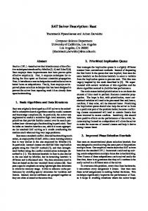
The Simulated Annealing algorithm [2] is applied using a temperature parameter of T . A generated neighbor assignment is accepted if it does not worsen the overall value of the current solution, or with the following probability paccept = e−T /∆ where ∆ is the increase in the overall value of the current solution when a detrimental move is assigned. The temperature T starts at initial value of SAit . It is cooled down (multiplied by cooling rate SAcr ) after each SAcc · T L iterations (SAcc is a cooling coefficient), where T L is an instance specific number (temperature length), computed as the sum of domain sizes of all variables. If the best solution found is not improved after SArc · SAcc · T L iterations (SArc is a reheat coefficient), temperature is increased to T = T · SAcr −1.7·SArc In the case when simulated annealing is used, the great deluge phase is stoped after the bound B reaches its lower limit and control is passed to the simulated annealing phase. Similarly, control is passed from the simulated annealing phase back to to hill climbing phase just after the temperature is reheated (see Figure 1). When simulated annealing is not used, control is never passed from the great deluge phase (GD continues immediately after the bound is increased).
8
Fig. 1. Algorithm schema when Simulated Annealing is used.
4
Competition Tracks
Value settings for the algorithm parameters used in each of the three competition tracks are listed in Table 1. Simulated annealing as not used on the examination timetabling problem for reasons discussed below. As is mentioned above, in Table 1. Solver parameters for each competition track
Parameter
Track 1
Track 2
Track 3
HCidle GDub GDlb GDcr SAit SAcr SAcc SArc
25,000 1.12 0.90 1 1 − 9·10 6
50,000 1.10 0.90 1 1 − 5·10 6 1.5 0.97 5 7
50,000 1.15 0.90 1 1 − 7·10 6 2.5 0.82 7 7
the hill climbing, great deluge, and simulated annealing phases, an assignment change (neighbor assignment) is randomly generated from a set of problem specific neighborhoods. Only moves that do not violate any hard constraints are generated. The first step is selection of a neighborhood. This neighborhood is then used to generate a change that is assigned if accepted by the currently used search strategy (HC, GD, or SA). The individual neighborhoods used in each of the tracks are described below. 4.1
Track 1: Examination Timetabling
The following neighborhoods are selected with equal probability during examination timetabling. All of the proposed neighborhoods attempt to change an assignment of an exam or to swap the periods and/or rooms of two exams. If a change cannot be made, it systematically searches for an alternate change by selecting the next feasible assignment that follows the initially proposed change
9
(i.e., it tries to use one of the subsequent periods or rooms in the variable’s domain in the order they are loaded from the input file) rather than randomly generating and checking of some other change. Exam swap An examination is randomly selected. A new period and room are randomly selected. If there is no (hard) conflict as a result of assigning the selected exam into the new period and room, the new assignment is returned. If there is only one conflicting examination, and it is possible to swap the selected examination with it, such a swap is returned. Following rooms and periods are tried otherwise (all rooms are first considered for the selected period, then for the next period, etc.). Only periods and rooms that are valid for the selected exam are considered. Period change An examination and a new period are randomly selected. If no conflict results from assigning the selected exam to the new period (keeping its room assignment), the new assignment is returned. Following periods are tried otherwise. The first available period is returned, another neighborhood is tried if no such period can be found. Room change An examination and a new room are randomly selected. If no conflict results from assigning the selected exam into the new room (keeping its period assignment), the new assignment is returned. Following rooms are tried otherwise. Period swap An examination and a new period are randomly selected. If just one conflict results from assigning the selected exam to the new period (keeping its room assignment), and it is possible to swap these two exams (each keeping its room assignment and taking the period assignment of the other exam), such a swap is returned. Following periods are tried otherwise. Room swap An examination and a new room are randomly selected. If just one conflict results from assigning the selected exam into the new room (keeping its period assignment), and it is possible to swap these two exams (each keeping its period assignment and taking the room assignment of the other exam), such a swap is returned. Following rooms are tried otherwise. Period and room change An examination and a new period are randomly selected. If no conflict results from assigning the selected exam to the new period (into a randomly selected available room), the new assignment is returned. Following periods are tried otherwise. The examination timetabling solver does not use the simulated annealing phase. Generation of the above described neighbor changes takes much more
10
time than in other tracks due to the complexity of the imposed soft constraints. When combined with the imposed time limit for each instance, various test runs indicated that the time is better spent using only the great deluge approach. 4.2
Track 2: Post Enrollment based Course Timetabling
In order to be able to find a complete solution quickly, soft constraints are ignored during the construction phase. Also, unlike in other tracks, it is allowable to assign an event to a time slot without assigning it into a room (e.g., in the case where there is no room available at the proposed time), or to violate a precedence constraint. Both the case of no room assignment and the violation of precedence constraints are treated as soft constraints. The algorithm starts with the weight of these soft constraints being one (overall solution value is the given score plus the weighted sum of violated no-room and precedence constraints), and these weights are increased by one after every 1,000 iterations during which there is no improvement in the number of violations of these constraints. This helps the solver to gradually decrease the number of these violations while it looks for the best solution score. The following neighborhoods are used during post enrollment based course timetabling (all are selected with the same probability, except of Precedence 1 the likelihood of the others). Swap which is selected with 10 Time Move An event and a new time slot are selected randomly. If it is possible to reassign the event into the new time slot while keeping its room without any conflict, such an assignment is returned. Following time slots are tried otherwise, with the first available time slot being returned if any are available. Room Move An event and a new room are selected randomly. If it is possible to reassign the event into the new room while keeping its current time assignment without any conflict, such an assignment is returned. Following rooms are tried otherwise, with the first available room being returned if any are available. Only rooms that are valid for the selected event are considered (i.e., rooms that are of sufficient size and that have all the required features). Event Move An event is randomly selected. A new time slot and a room are randomly selected. If there is no conflict in assigning the selected event into the new time and room, such an assignment is returned. If there is exactly one event conflicting with the new assignment and it is possible to swap these events, this swap is returned. Otherwise, it tries to use one of the following time slots and rooms (first it keeps the selected time slot and picks another room, then the same with the following time slot, etc.). Event Swap Two events are randomly selected. If it is possible to swap these two events, such a swap is retuned. Otherwise it tries to swap the times but pick a different room for these events (in a similar way as Room Move).
11
Precedence Swap This neighborhood tries to decrease the number of violated precedence constraints by reassigning an event into a different time and room. A violated precedence constraint is selected randomly, one of its events (randomly selected) is placed in a different time and room that does not violate the selected constraint. The time and room are picked in the same way as in Event Swap neighborhood. If no time and room can be found for the selected event, an attempt is made to move the other event as well. 4.3
Track 3: Curriculum based Course Timetabling
The following neighborhoods are used during the curriculum based course timetabling. All are selected with the same probability, except for Curriculum Com1 the likelihood of the others. pactness Move which is selected with 10 Time Move A period is changed for a randomly selected lecture. The first non-conflicting period after a randomly selected one is used. Room Move A room is changed for a randomly selected lecture. The first non-conflicting room after a randomly selected one is returned. Lecture Move A lecture is selected randomly, a new time and room are selected for the lecture. If no conflict results from assigning the selected lecture into the selected time and room, the assignment is returned. If there is another lecture conflicting with the time and room and it is possible to swap these two lectures, this swap is returned. Following times and rooms are tried otherwise. Only times that are available for the course of the selected lecture are considered. Room Stability Move This neighborhood tries to find a change that decreases the room stability penalty. A course and a room are selected randomly. An attempt is made to assign all lectures of the course into the selected room. If there is already another lecture in the room, it is reassinged to the room of the lecture being moved. Min Working Days Move This neighborhood tries to find a change that decreases course minimum working days penalty. A course with a positive penalty is selected randomly, a day on which two or more lectures are taught is selected, and one of lectures of that day is moved to a day that the course is not being taught on. Curriculum Compactness Move This neighborhood tries to find a change that decreases the curriculum compactness penalty. A curriculum is selected randomly, a lecture that is not adjacent to any other in the curriculum is selected and placed into another available period that has an adjacent lecture in the curriculum (if such placement exists and does not create any conflict). A different room may also be assigned to the lecture if the current one is not available.
12
5
Results
The following results were achieved using the above described solver. The tables below present results for all three tracks of the competition, computed within the given time limit, including early and late instances. The best solutions of 100 runs of each instance are presented.
Table 2. Results of Track 1 (Examination Timetabling)
Instance Number
1
2
3
Two Exams in a Row 42 0 1275 Two Exams in a Day 0 10 2070 Period Spread 2534 0 5193 Mixed Durations 100 0 0 Larger Exams Constraints 260 380 840 Room Penalty 1150 0 0 Period Penalty 270 0 190 Overall Value
4
5
6
7
8
7533 40 3700 0 0 3245 0 0 0 0 3958 1361 19900 3628 6718 0 0 75 0 0 105 1440 375 460 380 0 0 1250 0 125 1750 100 475 0 342
4356 390 9568 16591 2941 25775 4088 7565
Table 3. Results of Track 3 (Curriculum based Course Timetabling)
Instance Number
1 2 3 4
Room Capacity Minimum Working Days Curriculum Compactness Room Stability
4 0 0 1
Overall Value
5 43 72 35 298 41 14 39 103 9 0 331 66 53
0 15 28 0
0 10 62 0
5 6 7 8
0 0 0 0 5 180 15 0 30 114 26 14 0 4 0 0
9 10 11 12 13 14
0 0 0 0 0 0 0 5 35 5 0 255 10 5 34 68 4 0 76 56 48 0 0 0 0 0 0 0
All results have zero Distance to Feasibility (i.e., a complete feasible solution was found), except for one instance of Track 2 (Post Enrollment based Course Timetabling), see Table 4 for more details.
13 Table 4. Results of Track 2 (Post Enrollment based Course Timetabling)
Instance Number
4
5
6
7 8
Distance to Feasibility 0 0 0 0 More than Two in a Row 728 1093 73 111 One Class on a Day 23 21 132 283 Last Time Slot of a Day 579 1040 0 0
0 0 0 0
0 8 0 5
0 2 3 0
Overall Value
0 13
Instance Number
6
1
2
3
1330 2154 205 394 9
0 0 0 0
5 0
10 11 12 13 14 15 16
Distance to Feasibility 0 57 0 0 0 More than Two in a Row 881 1268 118 169 70 One Class on a Day 16 33 177 233 1 Last Time Slot of a Day 998 1139 52 51 3
0 2 0 0
0 0 0 0
Overall Value
2
0 6
1895 2440 347 453 74
0 2 4 0
Conclusion
At this point, it is hard to estimate how successful the presented approach will be. However, the comparison with other solvers will be quite valuable, especially since the same solver was used for all three tracks of the competition. This provides an opportunity to test the quality of solutions that can be achieved using a general approach to timetabling problems. Given that the presented approach is built on a framework and techniques that are currently being used to solve real, large-scale course timetabling problems, the results will also help in evaluating the effectiveness of the solver for these applications. Various test runs with different solver settings and other changes to the above described neighborhoods were performed. The above described algorithm and its parameters represent the best achieved results. However, it is likely that there is still plenty of room for optimization of the solver behavior and parameters. For more information about the presented approach, including source codes, please visit http://www.unitime.org/itc2007.
References [1] G. Dueck. New optimization heuristics: The great deluge algorithm and the recordto record travel. Journal of Computational Physics, 104:86–92, 1993. [2] S. Kirkpatrick, C. D. Gelatt, and M. P. Vecchi. Optimization by simulated annealing. Science, Number 4598, 13 May 1983, 220, 4598:671–680, 1983. [3] Tom´ aˇs M¨ uller. Constraint solver library. GNU Lesser General Public License, SourceForge.net. Available at http://cpsolver.sf.net. [4] Tom´ aˇs M¨ uller. Constraint-based Timetabling. PhD thesis, Charles University in Prague, Faculty of Mathematics and Physics, 2005.
14 [5] Tom´ aˇs M¨ uller, Roman Bart´ ak, and Hana Rudov´ a. Conflict-based statistics. In J. Gottlieb, D. Landa Silva, N. Musliu, and E. Soubeiga, editors, EU/ME Workshop on Design and Evaluation of Advanced Hybrid Meta-Heuristics. University of Nottingham, 2004. [6] Keith Murray, Tom´ aˇs M¨ uller, and Hana Rudov´ a. Modeling and solution of a complex university course timetabling problem. In Edmund Burke and Hana Rudov´ a, editors, Practice And Theory of Automated Timetabling, Selected Revised Papers, pages 189–209. Springer-Verlag LNCS 3867, 2007. [7] H. Rudov´ a T. M¨ uller, R. Bart´ ak. Minimal perturbation problem in course timetabling. In Edmund Burke and Michael Trick, editors, Practice And Theory of Automated Timetabling, Selected Revised Papers, pages 126–146. Springer-Verlag LNCS 3616, 2005.