Iteration at Different Levels: Multi-Level Methods for Structured Markov Chains Peter Buchholz Informatik IV, Universit¨at Dortmund D-44221 Dortmund, Germany email:
[email protected]
1
Introduction
Markov models are an established model type to describe systems from various application areas, including computer systems and networks, communication systems, biological systems, social systems and are also used to compute the page rank of Web pages and related measures. We consider here Markov chains with a finite state space RS = {0, . . . , n − 1}. Very often the stationary distribution is needed resulting in the solution of the set of equations πQ = 0 and πeT = 1 (1) in the continuous case and in the eigenvector computation πP = π
(2)
in the discrete time case [23]. In the former case Q is assumed to be an irreducible generator matrix and in the latter case, P is an irreducible stochastic matrix. It is well known that Q = (P − I) transforms a discrete time model into a continuous time model with the same stationary distribution and P = Q/α + I with α ≥ maxx∈RS |Q(x, x)| transforms a continuous time model into a discrete time model with the same stationary distribution. We will consider in this short note Markov processes in continuous time and since we only consider stationary analysis, the transformation from discrete to continuous time is straightforward. The major problem of computation of the stationary distribution for real examples is the size of the state space which can be several hundreds of millions or even billions of states. Thus, space and time efficient solution techniques are of major importance. The first step in developing more efficient analysis techniques is usually the finding of some structure for the state space. A common approach which naturally fits to many descriptions of real world examples is a multi-dimensional structure. Let J = {1, . . . , J} be the set of component indices and let RS (j) = {0, . . . , n(j) −1} be the set of states 1 Dagstuhl Seminar Proceedings 07071 Web Information Retrieval and Linear Algebra Algorithms http://drops.dagstuhl.de/opus/volltexte/2007/1059
in dimension j or the states of component j, then PS = ×Jj=1 RS (j) is the set of potentially reachable states in the composed model and if the transition rates are composable and PS equals RS the set of reachable states, then the generator matrix can be represented as J J X O O (j) (j) ˆ = Q λt Dt Et − (3) t∈T
j=1
j=1
where T is the set of model transitions and λt is the transition rate of (j) (j) transition t which might as well be included in one of the matrices Et . Et is the matrix describing the effect of transition t at component/dimension (j) (j) j and Dt = diag(Et eT ) is a diagonal matrix including the row sums (j) ˆ can in principle be used for the computation of the of Et . Matrix Q transient or stationary solution vector as first noticed for a slightly more general class of automata networks by Plateau [21]. In particular, it is ˆ using the possible to compute the product of a vector and the descriptor Q Kronecker representation from (3) rather than building the huge matrix. The disadvantage of (3) is that PS is usually much larger than RS since it contains unreachable states. To avoid this problem an additional dimension is introduced resulting in hierarchical matrices [6, 11]. For a hierarchical representation the state space RS is decomposed into global macro states such that matrix Q is structured into blocks Q1,1 · · · Q1,˜n .. .. Q = ... (4) . . Qn˜ ,1 · · · Qn˜ ,˜n
where n ˜ is the number of global macro states. Diagonal submatrices describe transitions inside global macro states and non diagonal matrices transitions between global macro states. According to the global macro states, each state space RS (j) is decomposed into subsets of states that belong to a global macro state. We denote these subsets as local macro states. A submatrix Qk,l can then be represented as !! J J N P N (j) (j) λt Et [jk , jl ]− δ(k = l) . (5) Dt [jk , jl ] Qk,l = t∈T
j=1
j=1
Here jk is the local macro state of component j in the global macro state k and submatrices include transitions between states belonging to the local macro states jk and jl . The representation Q is very compact since involved matrices are of order n(j) (jk ) rather than Jj=1 n(j) (jk ) where n(j) (jk ) is the number of detailed states in the local macro state jk belonging to global macro state k. Hierarchical matrices can be generated automatically at the model [10, 12] or state space level [8]. The hierarchical matrix representation 2
can be extended to discrete time models as shown in [7] for queuing networks in discrete time. It is straightforward to realize iterative solution techniques in conjunction with the compact matrix representation [1]. However, due to the state space size the solution time is often prohibitive such that more efficient approaches are required.
2
Multi Level Techniques
To speed up convergence of iterative methods so called multi level techniques have been proposed in various application areas [13]. The idea of all these approaches is to define a set of related iteration schemes considering different levels of detail, perform iterations at each level and transfer the improved or smoothed iteration vector from one level to another. For Markov chain problems, the approaches are often based on aggregation-disaggregation and use only two level [16, 20, 23]. However, also some aggregation/disaggregation approaches for more than two levels exist [2, 9, 15, 24]. In the sequel we present an extended version of the approaches proposed in [2, 9]. For any multi-level method, the following decisions have to be made: 1. How to define levels and how to transfer results from one level to another. 2. How to perform iterations at the different levels and how to define a complete iteration scheme. We begin with the definition of different levels and their interaction and present afterwards the complete algorithm. Finally very briefly some results are shown.
2.1
Definition of Levels
For models resulting from the composition of components every state from RS can be represented by a J-dimensional vector x = (x(0), . . . , x(J)) such that x(j) ∈ RS (j) . We define the most detailed or finest level by distinguishing all states from RS. A natural way of defining coarser levels is to use subsets C ⊂ J such that two states x = (x(0), . . . , x(J)) and y = (y(0), . . . , y(J)) are indistinguishable at the coarser level if and only if x(i) = y(i) for all i ∈ C and x(0) = y(0). Observe that the block level, component zero in each vector is not included in any subset such that only states from the same block are possibly mapped on the same aggregated state. Thus, C = ∅ results in a mapping where all states from one block are mapped on the same state. To generalize the approach define C ⊂ D ⊆ J . We use the subset as index to describe vectors and matrices at some level. I.e., RS C , QC and π C 3
are the state space, generator matrix and stationary solution vector of the Markov chain at the level defined by the detailed consideration of component states from the set C. A mapping from RS D into RS C is defined by a matrix RD,C with |RS D | rows and |RS C | columns. Such that for two states xD = [x(i)]i∈D and yC = [y(j)]j∈C , RD,C (xD , yC ) = 1 if x(j) = y(j) for all j ∈ C and RD,C (xD , yC ) = 0 otherwise. Observe that RD,C has row sum 1 and contains elements 0 or 1. Furthermore RJ ,C = RJ ,D RD,C . Matrix R. is denoted as restriction operator. It is independent of the current solution −1 (y) = {x|RD,C (x, y) = 1} for y ∈ RS C . or iteration vector. Let rC,D To map results from a coarse level RS C to a finer level RS D , a prolongation or projection operator is defined which is a matrix PC,D with |RS C | rows and |RS D | columns. PC,D is defined as a non negative matrix with row sum 1 such that PC,D (y, x) > 0 implies RD,C (x, y) = 1. The relation RD,C PC,D = I holds. There are two possibilities to define projection operators. The first is to define a constant matrix (see e.g. [24]), the second is to define matrix P. depending the current solution vector at RS D . Let pD some estimate of the solution vector at this level, then ( P −1 pD (x)/ z∈r−1 (y) pD (x) if x ∈ rC,D (y) , C,D (6) PC,pD (y, x) = 0 otherwise . With the restriction and prolongation operators Markov chains at the different levels can be defined. Assume that pD and QD are an approximation of the stationary vector and the generator matrix of a Markov chain with state space RS D . Then a mapping of the approximation and the generator matrix over state space RS C can be defined as follows. pC = pD RD,C and QC = PC,D QD RD,C
(7)
Instead of PC,D , also PC,pD may be used. The following two theorems are proved in [5]. Theorem 2.1 If QD is an irreducible generator matrix, the prolongation matrix contains one non zero element in each column and C ⊂ D, then QC is an irreducible generator matrix. If pD > 0, then PC,pD contains one non zero element per column. Thus, if QJ is irreducible, we only need to assure p. > 0 and use a prolongation matrix depending on p. as defined in (6) at each level to generate irreducible generator matrices at each level. Theorem 2.2 If π D is the stationary solution vector of the Markov chain with generator matrix QD and QC is computed using prolongation matrix PC,π D , then π D RD,C is the stationary solution vector of the Markov chain with generator matrix QC . 4
If QJ has a Kronecker representation as in (4) and (5), then every aggregated matrix QD has a Kronecker representation that includes only matrices for automata with indices from D and some vectors. For details see [2, 9].
2.2
The Iteration Scheme
In general there are different possibilities to define multi-level iterations. Using the notation of [5] the iteration matrix of the multi-level approach can be represented in a recursive form. Let D1 ⊂ D2 ⊂ . . . ⊂ DK = J be a set of nested component index sets. The following recursive description defines the multi-level iteration matrix for k > 1. ν2 ν1 ML L TM Dk = (TDk ) RDk ,Dk−1 TDk−1 PDk−1 ,pDk (TDk )
(8)
Here TDk is the iteration matrix at level Dk which might be the iteration matrix of the Power method (i.e., TDk = QDk /α+I for α ≥ maxx∈RS Dk |QDk (x, x)|), JOR or SOR. ν1 and ν2 are the numbers of pre- and post-iterations and pD is the iteration vector after the pre-iterations have been performed. For the ν0 L T coarsest level D1 we define TM D1 either as TD1 or as e π D1 where π D1 is the (k)
(k−1)
L is denoted stationary vector of QD1 . An iteration step pj = pj TM J as a cycle. Equation (8) describes the V-cycle of the multi-level method using a prolongation operator that depends on the current solution iteration vector. It is, of course, also possible to use a constant prolongation matrix. Similarly, W- oder F-cycles can be defined for the multi level approach. Apart from the choice of a cycle type and a prolongation operator, there are still two additional issues. First, how to define nested sets of component indices and second, how to choose ν1 and ν2 . A natural way of defining levels is to remove one component in each step. This results in J levels. In principle J! different orderings exist in which components can be removed and the ordering may even change from cycle to cycle. Typical orderings are fixed orderings where in every cycle indices are removed in the same order, a circular ordering where between the cycles component indices are cyclically shifted and dynamic ordering where indices are reordered between two cycles according to an estimate of the local error in the corresponding dimension. The number of pre- and post iterations can be fixed or it can depend on the convergence behavior. In the latter case let rD = pD QD the residual vector at level D. Then ν1 and ν2 may be set dynamically such that in each cycle at each level the norm of the residual vector is reduced. Since QD is an irreducible generator matrix under the conditions given above, the Power method assures that convergence at every level can be reached.
5
2.3
Example Results
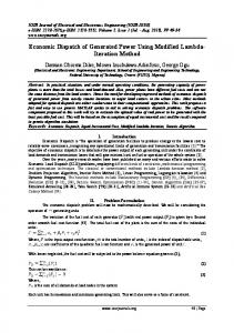
Since a proof of the convergence speed of the multi-level approach seems to be hard to achieve, one has to use empirical results to compare it with other solution techniques. A fairly large set of example results is presented in [4]. Here we only show results for two examples and summarize some general observations. Method Power ML(Power, fixed, 1, 1) SOR ML (SOR, fixed, 1, 1) BiCGStab (Pre. BSOR)
Iterations 79, 060 164 9590 20 390
CPU time in sec. 448.3 3.1 92.1 0.5 9.2
krk∞ 9.988e − 9 9.019e − 9 9.928e − 9 8.439e − 9 1.946e − 8
Table 1: Results for different solution methods applied to the example with ncd property. The first example is a queuing network example with loosely coupled submodels. A job performs a cycle of operations at different queues and changes the component at the end of a cycle with a probability 1%. This model has a mild NCD-property [23]. Out specific configuration consists of 4 components and results in a Markov chain with about 50, 000 states. Table 1 contains the results for this example. We show the required number of iterations and count for the multi-level methods only outer iterations. Furthermore, the CPU time and the residual norm after termination of the algorithms is presented. Five different solution techniques are compared. The Power method and SOR as conventional iterative methods [23], BiCGStab with a BSOR preconditioner [3] as a projection method and two multi-level variants using the Power method and SOR as smoother and 1 pre- and post-iteration per cycle. Form the results it is obvious that the multi-level methods clearly outperform the other solution methods. Method Power ML(Power, circular, 1, 1) SOR ML (SOR, circular, 1, 1) BiCGStab (Pre. BSOR)
Iterations 3, 990 892 140 50 40
CPU time in sec. 3502.0 1227.0 162.5 87.8 210.6
krk∞ 9.263e − 9 9.734e − 9 3.062e − 9 2.450e − 9 5.886e − 9
Table 2: Results for different solution methods applied to the courier protocol example. The second example we consider is a stochastic Petri net model describing two layers of a simple client server protocol [25]. The configuration we analyzed results in a Markov chain with 1, 632, 600 states. For this example 6
the different components are strongly coupled. However, as one can see from the results in table 2, multi-level methods with a circular ordering of components to be aggregated still outperform other solution methods although the difference is not as large as for the previous example. From our fairly comprehensive set of example runs in [4] we draw the following conclusions: • Multi-level methods are for almost all models we analyzed the fastest solvers. The speedup of multi-level methods compared to other iterative methods can be several orders of magnitude if components are loosely coupled. • A small and fixed number of pre- and post-iterations seems to be the best choice. • SOR is often the best choice as a smoother. • The difference between the three cycle types is relatively small. • Among the ordering of aggregation we tried, a fixed ordering seems to be the most robust choice, whereas a circular or dynamic ordering depending on the local residual is often more efficient. • A prolongation operator depending on the current iteration vector gave much better results than a static prolongation operator. With a static prolongation operator, the multi-level approach was often not faster than the basic iteration method without multi-level steps. • Multi-level approaches may be used as preconditioners for prolongation methods. Our experience is that the approach does not work with prolongation operators depending on the iteration vector and for fixed projection operators we obtained no speed up compared to the projection method without preconditioning.
3
What about Page Rank?
The matrices that are used in the previous section result from a multi dimensional description such that levels follow naturally from the definition of the model. For most Markov chains for information retrieval including the Google matrix [17] such a structure does not exist. However, one can try to approximate the matrix by a structured matrix. Some results about reordering the Google matrix to a form with strongly coupled blocks exist [18] and also first applications of two level methods to the compute page rank exist [19]. To apply the multi level approach presented here to general stochastic matrices P, one has to define a block decomposition such that every block 7
can be approximated by a sum of Kronecker products of matrices. I.e., the goal is to find a substochastic matrix A such that A has a Kronecker representation similar (4), (5) and P = A + D where the elements of D are non negative and small compared to the elements of A. Usually A needs not be irreducible since P is not irreducible. For the computation of the stationary vector, the matrix αP + (1 − α)evT is used where v is the personalization vector (see [17] for details). If matrix A has been found, then the multi-level approach can be applied using the following iteration scheme. p(k) (A − I)M L = b where b = −p(k−1) D
(9)
In contrast to the solution of structured Markov chains the multi level approach now has to be applied for a system with non zero right hand side which can be done without problems. It remains to find an approximate matrix A which is the hardest problem. The goal is to find for some submatrix B of A two matrices B1 ⊗ B2 such that B ≈ B1 ⊗ B2 . Several approaches exist to approximate matrices by Kronecker products of matrices [14, 22] and may be applied for this purpose.
4
Conclusions and Open Research Questions
Multi-level approaches as an adaption of algebraic multi-grid methods to continuous time Markov chains have shown to be very efficient solvers which outperform other iterative techniques for most examples. However, multilevel methods define a class of methods rather than a single method. A large number of parameters is available for these methods which all have some influence on the performance of the resulting solver. Currently, it is still an open research question how to set these parameters to obtain an optimal or nearly optimal solver for a given problem. To exploit the full potential of multi-level methods, adaptive steps have to integrated to set the parameters of the method according to the observed convergence speed. It has been shown that a multi level structure is naturally given for most models for performance or dependability analysis, but it is usually not available for Markov chains resulting from Web graphs. To exploit structured solution methods also to those Markov chains, the resulting matrices have to be represented or approximated by a sum of Kronecker products of small matrices. It has been outlined how such a representation may be found, but algorithms for this purpose are still missing.
References [1] P. Buchholz. Structured analysis approaches for large Markov chains. Applied Numerical Mathematics, 31(4):375–404, 1999. 8
[2] P. Buchholz. Multi-level solutions for structured Markov chains. SIAM Journal on Matrix Methods and Applications, 22(2):342–357, 2000. [3] P. Buchholz and T. Dayar. Block SOR preconditioned projection methods for Kronecker structured Markovian representations. SIAM Journal on Scientific Computing, 26:1289–1313, 2005. [4] P. Buchholz and T. Dayar. Experimental comparison of structured analysis techniques for large Markov chains. Technical Report Forthcoming Technical Report, Universit¨at Dortmund, Fachbereich Informatik, 2007. [5] P. Buchholz and T. Dayar. On the convergence of a class of multilevel methods for large sparse Markov chains. SIAM Journal on Matrix Methods and Applications, to appear 2007. [6] Peter Buchholz. A hierarchical view of gcspns and its impact on qualitative and quantitative analysis. J. Parallel Distrib. Comput., 15(3):207– 224, 1992. [7] Peter Buchholz. On the exact and approximate analysis of hierarchical discrete time queueing networks. In Heinz Beilner and Falko Bause, editors, MMB, volume 977 of Lecture Notes in Computer Science, pages 150–164. Springer, 1995. [8] Peter Buchholz. Hierarchical structuring of superposed gspns. IEEE Trans. Software Eng., 25(2):166–181, 1999. [9] Peter Buchholz and Tugrul Dayar. Comparison of multilevel methods for kronecker-based markovian representations. Computing, 73(4):349– 371, 2004. [10] Peter Buchholz and Peter Kemper. On generating a hierarchy for gspn analysis. SIGMETRICS Performance Evaluation Review, 26(2):5–14, 1998. [11] Peter Buchholz and Peter Kemper. Kronecker based matrix representations for large markov models. In Christel Baier, Boudewijn R. Haverkort, Holger Hermanns, Joost-Pieter Katoen, and Markus Siegle, editors, Validation of Stochastic Systems, volume 2925 of Lecture Notes in Computer Science, pages 256–295. Springer, 2004. [12] Javier Campos, Susanna Donatelli, and Manuel Silva. Structured solution of asynchronously communicating stochastic modules. IEEE Trans. Software Eng., 25(2):147–165, 1999. [13] Robert D. Falgout. An introduction to algebraic multigrid. Computing in Science and Engineering, 8(6):24–33, 2006. 9
[14] M. P. Friedlander and K. Hatz. Computing nonnegative tensor factorizations. Technical Report TR-2006-21, Dep. of Comp. Sci., University of British Columbia, 2006. [15] Graham Horton and Scott T. Leutenegger. A multi-level solution algorithm for steady-state markov chains. In SIGMETRICS, pages 191–200, 1994. [16] U. Krieger. Numerical solution of large finite Markov chains by algebraic multigrid techniques. In W. J. Stewart, editor, Computations with Markov chains, pages 403–424. Kluwer Academic Publishers, 1995. [17] A. Langville and C. D. Meyer. A survey of eigenvector methods for web information retrieval. SIAM Review, 47(1):135–161, 2005. [18] A. N. Langville and C. D. Meyer. A reordering for the PageRank problem. Technical report, Dep. of Mathematics, N. Carolina State University, 2004. [19] C. Pan-Chi Lee, G. H. Golub, and S. A. Zenios. A fast two-stage algorithm for computing PageRank and its extensions. Technical Report SCCM-03-15, Dep. of Comp. Sci., Stanfort University, 2003. [20] I. Marek and P. Mayer. Convergence analysis of an iterative aggregation/disaggregation method for computing the probability vector of stochastic matrices. Numerical Linear Algebra with Applications, 5(4):253–274, 1998. [21] Brigitte Plateau. On the stochastic structure of parallelism and synchronization models for distributed algorithms. In SIGMETRICS, pages 147–154, 1985. [22] A. Shashua and T. Hazan. Non-negative tensor factorization with applications to statistics and computer vision. In Luc De Raedt and Stefan Wrobel, editors, ICML, pages 792–799. ACM, 2005. [23] W. J. Stewart. Introduction to the numerical solution of Markov chains. Princeton University Press, 1994. [24] E. Virnik. An algebraic multigrid preconditioner for a class of singular M-matrices. Preprint 03-2006, TU Berlin, 2006. [25] C. M. Woodside and Y. Li. Performance Petri net analysis of communications protocol software by delay equivalent aggregation. In Proc. 4th Int. Workshop on Petri Nets and Performance Models, pages 64–73. IEEE CS Press, 1991.
10