Iterative Abstraction-based CTL Model Checking Jae-Young Jang Motorola Inc., 7700 W. Parmer Lane Austin, TX 78729
[email protected]
In-Ho Moon Gary D. Hachtel University of Colorado at Boulder ECEN Campus Box 425 Boulder, CO 80309 In.Moon,Gary.Hachtel @colorado.edu
Abstract A paradigm for automatic approximation/refinement in conservative CTL model checking is presented. The approximations are used to verify a given formula conservatively by computing upper and lower bounds to the set of satisfying states at each sub-formula. These approximations attempt to perform conservative verification with the least possible number of BDD variables and BDD nodes. We present new forms of operational graphs to avoid limitations associated with previously used operational graphs. Three new techniques for efficient automatic refinement of approximate system are presented. These methods make it easier to find the locality. We also present a new type of don’t cares (Approximate Satisfying Don’t Cares) that can make model checking more efficient in time and space. On average, an order of magnitude speedup was achieved.
calls is quadratic in the number of subsystems in the system. This procedure is limited to CTL formulae. In [12], a more sophisticated, operation-based refinement was proposed. The given CTL formula is parsed, and the initial error states (initial states shown not to satisfy the given CTL formula) are treated as a “goal set.” Using the parse tree of the formula, called an operational graph, the goal set is systematically distributed for refinement to the operations which induced the approximation in the first place. This procedure requires exact image computation to propagate goal set. Another new method that uses upper- and lowerapproximations at the same time was introduced in [8]. But, they did not explore all the benefits from previously computed satisfying states (explained in Section 5) and their refinement method is only based on dependency relation with structural depth.
2. Approximation 1. Introduction The success of formal verification in detecting incorrect designs has been proven over the last decade. However, the limitation on the size of verifiable problems continue to be a serious drawback. Therefore, for most practical, industrial strength designs, abstraction, either manual or automatic, is required to make formal verification tractable. There has been extensive research on this topic. Some of works that were foundation of this research are summarized below. In [6], Kurshan described an abstraction paradigm called “localization reduction” in the context of -regular language containment based on reducing the parts of a system that are irrelevant with respect to the property being verified. Another approach using both (but not at the same time) over and under approximations was considered in [7] based on State Space Decomposition [3]. If the result is not conclusive due to abstraction, further refinement is done by adding the best subsystem to each of the remaining subsystems. In the worst case, the number of decision procedure
The physical interpretation of the given system is a finite state machine (FSM) model. Here the symbol X represents the external input to the system. We operate in an encoded world, so S 0 1 n and X 0 1 q, and s S denotes a nvector of state variable value assignments. To distinguish a present state s S from a next state s S t is used to express a state after one clock cycle from a state s. The triple s x t can be viewed as a member of the system transition relation T , or equivalently as a labeled edge of the State Transition n Graph. Thus there are n latches, and T i 1 Ti s x ti is the system transition relation. This transition relation can be implemented in many ways. In this research, BDDs are used to manipulate a set and a relation including T s x ti . In general, BDDs operations are exponential in the number of variables and polynomial in the size of BDDs nodes. Model checking of a CTL [4] property f is based on a states evaluation function, SAT f —all states in SAT f satisfy f [10]. After computation of SAT f , the initial states, S0 , are compared to SAT f and verification is com-
pleted with the following test: S0
SAT f
f istrue
(1)
Many researchers have focused on approximate evaluation of the set of satisfying states. We shall refer to two such approximate evaluating functions: SAT f , and SAT f : SAT
f
SAT f
SAT
f
When we derive exact verification results from these approximate states evaluations, we call it Conservative Verification ( Positive Conservatism: S0 SAT f S0 SAT f , Negative Conservatism: S0 SAT f S0 SAT f . All SAT f computations can be based on one primitive operation called PRE C s which computes predecessors of states in C s : PRE C s
T s x ti C t
xt
(2)
i I
Same index i I are associated with si ti , and Ti s x ti and Ti is used instead of Ti s x ti interchangeably. Of the many ways to implement upper-bound or lower-bound of Equation 2, we shall consider only the following methods defined in Definition 2.1 and 2.2, where Ti Ti Ti . With these methods, lower-bound and upper-bound preimage computations are defined as shown below. Here, C t is computed from C t according to the approximation method being used. PRE C t PRE C t
xt xt
T T
sxt C t sxt C t
Definition 2.1 (Upper-bound Transition Relation) T
sxt
Ti s x ti
Here, I A
I IR
(U1) Ti
I
Ti
1, C t
(3)
I A.
BddSupersetting Ti , C t
(U2) Ti
s x ti
i IR
i IA
tR C
t
, tR
Ct .
ti i
IR .
U1 refers to making Ti from Ti with generic BDDs supersetting techniques explained in [13]. These methods produce a new set that is close to the original set in terms of on-set minterm count, where the new BDDs should be much smaller in size. U2 refers to the Block Tearing Method [1, 9, 7], where Ti is the tautology. All t R variables are not appeared during PRE computation. Definition 2.2 (Lower-bound Transition Relation) T
sxt
Ti s x ti i IA
Ti i IR
s x ti
(4)
(L1) Ti
BddSubsetting Ti , C t
(L2) Ti
1, C t
tRC
t , tA
Ct . ti i
IA .
The L1 method is same as U1 but the complement of the given BDDs are supersetted. The L2 method was used in [7] to disprove a CTL formula more efficiently. All approximation methods explained in this section are easier than exact one in a sense that either the number of variables is reduced or the size of BDDs are reduced during PRE computation.
3. New Operational Graphs The notion of an Labeled Operational Graph was first defined in [12]. There a Polarity was associated with each node in operational graph. The polarity of a node of the operation graph tells whether over- (+) or underapproximation (-) should be computed at that node in order to have a positive conservative answer at the top node. However, it considered only the case of ‘-’ polarity at the top node, therefore, only Positive Conservatism was considered in that work. We now define a Dioecious Operational Graph (DOG), which allows either positive or negative polarity at the top node. We shall refer to a graph with a required ‘+’(‘-’) polarity at the top as a Positive (Negative) Dioecious Operational Graph, pDOG (nDOG) respectably. Then the Labeled Operational Graph in [12] is same as nDOG. Note that a model checker requires a pDOG in order to deal with Negative Conservatism. Since pDOG or nDOG has a one-side advantage (e.g., f with nDOG is good to conservatively verify f TRUE, but not for verifying f FALSE), we should exploit the advantage of both cases. If nDOG and pDOG are merged, a more effective approximate verification approach can be achieved without causing too much overhead. This operational graph shall be called the Monoecious Operational Graph (MOG). Every node v in MOG has SAT v and SAT v at the same time. With these two approximate satisfying states, dual conservatism can be applied on a unified labeled operational graph. The other benefit of MOG will be explained in Section 5. In Figure 1, three different operational graphs of AG EFq are illustrated. First, formula f should be translated into CTL form by using equivalence rules explained in [10]. For example, AGp EU True p and EFq EU True q . The polarity of a given node v in DOG is determined by counting the number of nodes in a path from the top node to v. When even number of nodes in this path, node v gets the same polarity as the top node. SAT v or/and SAT v is computed according to a polarity of v in a operational graph in depth first order. It is guaranteed that an approximate satisfying set at the top node is correct by using this method [12].
4.1. Latch Affinity Refinement
Figure 1. Different Operational Graphs for AG EFq
4. Iterative Model Checking and Refinement In approximate CTL based model checking, the main operations are SAT f and SAT f computations. We compute SAT0 f or SAT0 f on the operational graph that we want to use first. If no conservative answer is found, SAT1 f or SAT1 f is computed with a refined system, where SAT0 f SAT1 f and SAT0 f SAT1 f . This process is continued until we prove the given formula or run out of gas. We call this type of verification Iterative Model Checking and the index i in SATi f is called iteration index. As the size of a circuit grows, it is more difficult to reason about it as a whole. So, most properties that we want to verify are written in a modular manner. In other words, a formula may require only part of a system to be verified by model checking. This is called Locality. In this sense, refinement is important because the main goal of refinement is how to find out the locality of a formula with less effort. In Equations 3 and 4, the index set I is divided into two sets, I A and I R . Then a transition sub-relation Ti for a state variable ti whose index i is in I R is approximated to Ti or Ti . The refinement is simply to replace Ti or Ti with Ti . Then, our problems are how to define I A and how to increase I A by adding I , a subset of I R . First, the constant bound is the size of I and defined by the user. The first index set I0 is computed as following. Let Id be a set of indices of latches shown in a given formula. If Id bound, IA I0 Id . Otherwise bound indices are chosen out of Id randomly. If the verification result is inconclusive, I A I A I1 and so on. To make refinement efficient, Ii should be computed in a way that Ii is more important to verify a given formula than any other combination of bound elements in I R . To compute Ii for i 0, the following two methods are used.
In [3], various relations between two latches were defined and used to partition the state space. Those relations are used here to compute efficient schedule to refine the approximate system. Those latch relations include connectivity, agreement, and affinity. The connectivity is computed based on whether a next state function depends on the other state variable. When two state variables have mutual dependency, their connectivity is 1. In case of uni-directional dependency, connectivity is 0.5 and 0 when there is no dependency. The aggrement shows how similar a next state function is to the other and the complement of the other. Minterm fraction of Exclusive OR of these two next state functions shows the similarity.Finally, the affinity is a convex combination of these two factors. Latch affinity is the factor that shows how two state variables are structurally dependent and how their behaviors are similar. Let i j be the affinity between si and s j . After computing I0 , the relational affinity j for each j I I0 is computed as below. ij
j
(5)
i I0
This new j is nothing but a summation of affinities between si in I0 and s j in I R . If j is bigger than k , it implies s j has stronger affinity to the state variables in the formula than sk . According to the relational affinity, we compute each Ii . This method is based on direct relations to the given formula.
4.2. Edge Traversal Refinement Upper-bound approximation creates pseudo edges which are not in the exact system. Main idea of this algorithm is to determine which transition sub-relation has more impact to delete them. Not every pseudo edges are considered, but the pseudo edges that are traversed from the initial states are targeted. First, a subset of initial states which have not been proved to satisfy the formula are propagated by pre-order depth first search in operational graph. This propagation, called Forward Edge Traversal is a series of upper-bound image computations bounded by SAT computed already. Each approximate image computation yields an edge envelope ee s x t which is a set of exact and pseudo edges. This edge envelope is conjoined with the negation of each transition sub-relation which is approximated during verification. This conjoined term is ee s x t Ti s x ti . The result is stored as Killi s x t and this is the set of edges to be removed if the approximated Ti s x t is replaced with exact Ti s x t . If any of Killi s x t is not empty during this propagation, the system is refined in a way that the transition sub-relation with the biggest minterm count
of Kill j s x t is refined. When no pseudo transition is found and the traverse reaches to bottom of the formula, then post-order propagation of refining procedure, called resolution propagation, where an un-verified set of states of a sub-formula during edge traversal is bi-partitioned into a set which satisfies the sub-formula and the other set where sub-formula is verified false. This second propagation verified the given formula. This refinement method is only applicable when all nodes v EXg EGg EU g h in operational graph have SAT v , because the edge envelope ee s x t is computed in SAT v . The advantages of this method are (1) refinement is guided by approximate satisfying states and (2) the impact can be predicted before the system is actually refined.
4.3. Example Now, a simple example is presented to illustrate the algorithms described in this section. The system models a 4-bit modulo 10 counter. States are encoded with variables counter 3 : 0 . The initial state is State 7 meaning ‘counter 3 : 0 0111’.
Figure 2. STGs of a 4-bits modulo 10 counter The specification that we want to check is f AG counter 3 : 0 1010 . The partial exact state transition graph is in (1) of Figure 4. Since state 10 does not have any predecessor, this formula is true. Let us now find out how approximation and refinement work. The ‘Universal quantification Method (L2)’ explained in Definition 2.2 is used for lower bound computation and the ‘Existential quantification Method (U2)’ in Definition 2.1 is for upper bound computation. Let us start with an initial approximate system which includes counter 3 : 2 . This approximation results in a new state transition graph (4) in Figure 4. The approximate system should be refined because no conservative answer can be derived from above results. First, let us apply Latch Affinity Refinement method. With this method, 0 0 5 (relational affinity to counter 0 ) and 1 1 0 (relational affinity to counter 1 ) as in Figure 3. Detail computation methods can be found in [3].
Figure 3. Relational Affinity graph of a 4-bits modulo 10 counter
Based on this factor, counter 1 is selected to refine the approximate system. The refined STGs (2) is changed from (4) in Figure 4. There is no reason to further refine because State 10 does not have preimage now and the formula f is verified true by positive conservatism. Now, Edge Traversal Refinement method is applied. Forward edge traversal computes the first ee s t 7 8 7 10 7 11 . There are two pseudo edges (7,10) and (7,11) in ee s t . Notice that these two edge contribute to make the formula f false because there are two paths, (7,10) and (7,11,2,3,4,5,6,7,8,10) which lead the initial state to State 10. The set of pseudo edges that can be killed by counter 1 and counter 0 are: killcounter 1 killcounter 0
7 10 7 11
7 11
This method also chooses counter 1 rather than counter 0 because killcounter 1 2 is bigger than killcounter 0 1. Both methods successfully refine and verify the formula f with three latches. If counter 0 is selected, all latches must be included to verify the formula f . This is because the edge (7,10) is not killed by adding counter 0 only.
5. Approximate Satisfying Don’t Care Reachability analysis of a system has a significant role in model checking. A set of reachable states is used to make transition relation smaller by RESTRICT [5] operation. This minimized transition relation is smaller than original one because unreachable states are used as don’t care states. This type of don’t cares is called Reachability Don’t Care(RDC). In [11], a superset of exact reachable
overhead is compensated with the reduction of the transition relation by ASDC. For instance, Example 7 in Table 6 is the case where pDOG used 63.9MB memory while MOG used 42.9MB only. Figure 5 shows how upper-bound satisfying states are used as care states to minimize transition relations in this Example. The average size of approximate transition relation minimized by ASDC is 20.08% of one without ASDC. 80000
Exact TR size without ASDC Upper TR size with ASDC Lower TR size with ASDC
70000
BDD size of Transition Realtion
Figure 4. Upper-bound approximate STGs of a modulo 10 counter with different T . Only part of the whole STG is shown. A dashed line is a pseudo edge. (1) T T3 T2 T1 T0 , (2) T T3 T2 T1 , (3) T T3 T2 T0 , (4) T T3 T2 .
states is computed and used in the same way. This is called Approximate Reachability Don’t Care (ARDC). The benefit of Iterative Verification is to use SATi v as don’t cares to minimize the transition relation and reduce the cost of computing the refined SATi 1 v or SATi 1 v . SAT v is called Approximate Satisfying Don’t Care(ASDC). This is possible because the refined system yields tighter satisfying states than previous level of approximate system for a given sub-formula v as below.
60000
50000
40000
30000
20000
10000
0 0
30
60
90 120 150 180 210 Number of latches in the approximate system
240
270
300
Figure 5. Minimization of T s x t by ASDC.
6. Experimental Results SAT i v
SATi
1
v
SATi
1
v
SATi v
(6)
In addition to the extra don’t cares, the fixpoint computation can be simplified by the following observation. When we compute the greatest fixpoint computation SATi 1 EG p as below, initially y is tautology. SATi
1
EG p
y SATi
1
p
PRE y
(7)
But, y SATi EG p can be used as the first computation and reduce some redundant steps because of 6. Also, when we compute the least fixed point of EF p , SATi EF p is used instead of a empty set by the same reason. Based on these two observations, upper-bound approximate satisfying set enables us to make upper and lower transition relations smaller and both upper- and lowerbound approximate satisfying sets reduce the number of iterations with tighter starting point. MOG enjoys these two benefits because every node in the operational graph has both approximations. Any node with only negative polarity in DOG can not use ASDC. Generally speaking, MOG’s overhead to compute both SAT and SAT requires more computing resources than DOG uses. But, as the approximate system gets refined close to the exact system, MOG’s
We have implemented all the algorithms in this paper in VIS-1.3 (called IMC). All experiments were ran on two different machines. The first one is a Pentium II(400MHz) system with 512K internal L2 cache and 1GB main memory. The other is a Pentium II(233MHz) system with 256K internal L2 cache and 256MB main memory. VIS-1.3 [2] was used as a main platform and CUDD-2.3.0 [14] was used. Here, RM: Refinement Method (S: Latch Affinity Method, D: Edge Traversal), OG: Operational Graph (M: MOG, P: pDOG, N: nDOG), FF: Number of latches in a circuit, RFF: Number of latches reduced by formula dependency, and VFF: I A . The results of IMC are compared to the ones from exact model checker (MC). Not every combination of lower-bound methods, upper-bound methods, and refinement methods were tested. But, many examples were chosen from a small circuit to a big one to demonstrate that incremental verification is not restricted to some class of the circuits. Example 4 through 12 were the best results among nDOG , pDOG and MOG . MOG was the best in 6 examples out 9. Example 3 is a case where ASDC helps model checking even though there is no locality and the approximate system should be increased to the exact system. For all 12 cases, average memory usage of IMC is less than 30.0% of MC (CPU Time is about 15%).
No 1 2 3 4 5 6 7 8 9 10 11 12
Circuit
FF
PDC Example1 Ethernet CPS Hw Top
61 115 118 231 356
TrainFlat
866
Avq
3705
Formula
T/F
AG(p AF q) AG(p AF q) AG(p AFq) AG(EF p) AG(EF p) AG(p EF q) AG(EF p) AG(p EF q) AG(p EF q) AG(EF p) AG(p EF q) EF p
T T T F F T F T T F T T
RFF 61 115 86 231 356 277 306 583 609 609 2715 2772
RM
OG
D D D S S S S S S S S S
N N N M P N M N M M M M
VFF 58 6 86 4 12 62 251 37 16 16 3 11
IMC MB 6.9 5.8 13.5 9.5 14.0 22.0 42.9 18.4 17.6 17.7 162.4 163.7
MC TIME 23 12 978 14 64 1409 299 536 207 203 668 922
MB 26.3 14.4 20.6 19.4 30.7 90.0 248.4 269.7 292.1 322.3 321.6 616.6
TIME 1751 1905 2506 956 182 3533 27600 1781 1846 4339 1932 86400
Table 1. Experimental results.
7. Conclusions In approximate model checking, there are two main goals. The first one is efficiency to find out the locality of a formula. The impact of this is significant because the number of BDD variables can be reduced by property locality. The second is how easier approximate computation is than exact one. In this paper, efficient refinement algorithms were introduced for the first goal. The upper-bound and lower-bound methods along with ASDC were proposed to achieve the second target. It is true that there is a formula that does not have any locality. For this kind of formula, the approximation method seems to be useless. But, thanks to ASDC, the verification with the last iteration index may be easier than the exact verification when ASDC is not empty. The impact of all these new ideas was demonstrated with big examples. Order of magnitude speedup was achieved with 70% reduction in memory consumption.
[5]
[6] [7]
[8]
[9]
[10]
References [1] F. Balarin and A. L. Sangiovanni-Vincentelli. An iterative approach to language containment. In C. Courcoubetis, editor, Fifth Conference on Computer Aided Verification (CAV ’93). Springer-Verlag, Berlin, 1993. LNCS 697. [2] R. K. Brayton et al. VIS: A system for verification and synthesis. In T. Henzinger and R. Alur, editors, Eigth Conference on Computer Aided Verification (CAV’96), pages 428–432. Springer-Verlag, Rutgers University, 1996. LNCS 1102. [3] H. Cho, G. D. Hachtel, E. Macii, M. Poncino, and F. Somenzi. A structural approach to state space decomposition for approximate reachability analysis. In Proceedings of the International Conference on Computer Design, pages 236–239, Cambridge, MA, Oct. 1994. [4] E. M. Clarke and E. A. Emerson. Design and synthesis of synchronization skeletons using branching time tempo-
[11]
[12]
[13]
[14]
ral logic. In Proceedings Workshop on Logics of Programs, pages 52–71, Berlin, 1981. Springer-Verlag. LNCS 131. O. Coudert, C. Berthet, and J. C. Madre. Verification of sequential machines using boolean functional vectors. In L. Claesen, editor, Proceedings IFIP International Workshop on Applied Formal Methods for Correct VLSI Design, pages 111–128, Leuven, Belgium, Nov. 1989. R. P. Kurshan. Computer-Aided Verification of Coordinating Processes. Princeton University Press, Princeton, NJ, 1994. W. Lee, A. Pardo, J. Jang, G. Hachtel, and F. Somenzi. Tearing based abstraction for CTL model checking. In Proceedings of the International Conference on Computer-Aided Design, pages 76–81, San Jose, CA, Nov. 1996. J. Lind-Nielsen and H. R. Anderson. Stepwise ctl model checking of state/event systems. In N. Halbwachs and D. Peled, editors, Eleventh Conference on Computer Aided Verification (CAV’99). Springer-Verlag, Berlin, 1999. D. E. Long. Model Checking, Abstraction, and Compositional Verification. PhD thesis, Carnegie-Mellon University, July 1993. K. L. McMillan. Symbolic Model Checking. Kluwer Academic Publishers, Boston, MA, 1994. I.-H. Moon, J.-Y. Jang, G. D. Hachtel, F. Somenzi, C. Pixley, and J. Yuan. Approximate reachability don’t cares for CTL model checking. In Proceedings of the International Conference on Computer-Aided Design, pages 351–358, San Jose, CA, Nov. 1998. A. Pardo and G. D. Hachtel. Automatic abstraction techniques for propositional -calculus model checking. In O. Grumberg, editor, Ninth Conference on Computer Aided Verification (CAV’97), pages 12–23. Springer-Verlag, Berlin, 1997. LNCS 1254. K. Ravi, K. L. McMillan, T. R. Shiple, and F. Somenzi. Approximation and decomposition of decision diagrams. In Proceedings of the Design Automation Conference, pages 445–450, San Francisco, CA, June 1998. F. Somenzi. CUDD: CU Decision Diagram Package. ftp://vlsi.colorado.edu/pub/.