Iterative Methods - Wiley

CHAPTER

1 Iterative Methods

Some things are simple but hard to do. —A. Einstein

Most of the problems in this book are simple. Many of the methods used have been known for decades or for centuries. At the machine level, individual steps in the procedures are at the grade school level of sophistication, like adding two numbers or comparing two numbers to see which is larger. What makes them hard is that there are very many steps, perhaps many millions. The computer, even the once ‘‘lowly’’ microcomputer, provides an entry into a new scientific world because of its incredible speed. We are now in the enviable position of being able to arrive at practical solutions to problems that we could once only imagine.

Iterative Methods One of the most important methods of modern computation is solution by iteration. The method has been known for a very long time but has come into widespread use only with the modern computer. Normally, one uses iterative methods when ordinary analytical mathematical methods fail or are too time-consuming to be

Computational Chemistry Using the PC, Third Edition, by Donald W. Rogers ISBN 0-471-42800-0 Copyright # 2003 John Wiley & Sons, Inc. 1

2

COMPUTATIONAL CHEMISTRY USING THE PC

practical. Even relatively simple mathematical procedures may be time-consuming because of extensive algebraic manipulation. A common iterative procedure is to solve the problem of interest by repeated calculations that do not initially give the correct answer but get closer to it as the calculation is repeated, perhaps many times. The approximate solution is said to converge on the correct solution. Although no human would be willing to repeat an iterative calculation thousands of times to converge on the right answer, the computer does, and, because of its speed, it often arrives at the answer in a reasonable amount of time.

An Iterative Algorithm The first illustrative problem comes from quantum mechanics. An equation in radiation density can be set up but not solved by conventional means. We shall guess a solution, substitute it into the equation, and apply a test to see whether the guess was right. Of course it isn’t on the first try, but a second guess can be made and tested to see whether it is closer to the solution than the first. An iterative routine can be set up to carry out very many guesses in a methodical way until the test indicates that the solution has been approximated within some narrow limit. Several questions present themselves immediately: How good does the initial guess have to be? How do we know that the procedure leads to better guesses, not worse? How many steps (how long) will the procedure take? How do we know when to stop? These questions and others like them will play an important role in this book. You will not be surprised to learn that answers to questions like these vary from one problem to another and cannot be set down once and for all. Let us start with a famous problem in quantum mechanics: blackbody radiation.

Blackbody Radiation We can sample the energy density of radiation rðn; TÞ within a chamber at a fixed temperature T (essentially an oven or furnace) by opening a tiny transparent window in the chamber wall so as to let a little radiation out. The amount of radiation sampled must be very small so as not to disturb the equilibrium condition inside the chamber. When this is done at many different frequencies n, the blackbody spectrum is obtained. When the temperature is changed, the area under the spectral curve is greater or smaller and the curve is displaced on the frequency axis but its shape remains essentially the same. The chamber is called a blackbody because, from the point of view of an observer within the chamber, radiation lost through the aperture to the universe is perfectly absorbed; the probability of a photon finding its way from the universe back through the aperture into the chamber is zero.

3

ITERATIVE METHODS

Radiation Density

Energy Density, J m –3

If we think in terms of the particulate nature of light (wave-particle duality), the number of particles of light or other electromagnetic radiation (photons) in a unit of frequency space constitutes a number density. The blackbody radiation curve in Fig. 1-1, a plot of radiation energy density r on the vertical axis as a function of frequency n on the horizontal axis, is essentially a plot of the number densities of light particles in small intervals of frequency space. We are using the term space as defined by one or more coordinates that are not necessarily the x, y, z Cartesian coordinates of space as it is ordinarily defined. We shall refer to 1-space, 2-space, etc. where the number of dimensions of the space is the number of coordinates, possibly an n-space for a many dimensional space. The r and n axes are the coordinates of the density–frequency space, which is a 2-space. Radiation energy density is a function of both frequency and temperature r(n,T) so that the single curve in Fig. 1-1 implies one and only one temperature. Because frequency n times wavelength l is the velocity of light c ¼ nl ¼ 2:998  108 m s1 (a constant), an equivalent functional relationship exists between energy density and wavelength. The energy density function can be graphed in a different but equivalent form r(l,T). The intensity I of electromagnetic radiation within any narrow frequency (or wavelength) interval is directly proportional to the number density of photons. It is also directly proportional to the power output of a light sensor or photomultiplier; hence both I and r are measurable quantities. Whenever one plots some function of radiation intensity I vs. n or l, the resulting curve is called a spectrum.

Frequency

Figure 1-1 The Blackbody Radiation Spectrum. The short curve on the left is a Rayleigh function of frequency.

4

COMPUTATIONAL CHEMISTRY USING THE PC

Wien’s Law In the late nineteenth century, Wien analyzed experimental data on blackbody radiation and found that the maximum of the blackbody radiation spectrum lmax shifts with the temperature according to the equation lmax T ¼ 2:90  103 m K

ð1-1Þ

where l is in meters and T is the temperature in kelvins.

The Planck Radiation Law As Lord Rayleigh pointed out, the classical expression for radiation
 rðn; TÞdn ¼ 8pkB T=c3 n2 dn

ð1-2Þ

where kB is Boltzmann’s constant and c is the speed of light, must fail to express the blackbody radiation spectrum because r ¼ const:  n2 is a segment of a parabola open upward (the short curve to the left in Fig. 1-1) and does not have a relative maximum as required by the experimental data. In late 1900, Max Planck presented the equation
 rðn; TÞdn ¼ 8phn=c3 n2

dn ehn=kB T  1

ð1-3Þ

where the units of rðn; TÞ are joules per cubic meter, as appropriate to an energy in joules per unit volume and h ¼ 6:626  1034 J s (joule seconds) is a new constant, now called Planck’s constant. This equation expressed in terms of wavelength l is
 rðl; TÞ dl ¼ 8phc=l5

dl ehc=lkB T

1

ð1-4Þ

By setting dr=dl ¼ 0, one can differentiate Eq. (1-4) and show that the equation x ex þ ¼ 1 5

ð1-5Þ

holds at the maximum of Fig. 1-1 where x¼

hc lkB T

Exercise 1-1 Given that c ¼ nl, show that Eqs. (1-3) and 1-4) are equivalent.

Exercise 1-2 Obtain Eq. (1-5) from Eq. (1-4).

ð1-6Þ

ITERATIVE METHODS

5

  COMPUTER PROJECT 1-1 Wien’s Law The first computer project is devoted to solving Eq. (1-5) for x iteratively. When x has been determined, the remaining constants can be substituted into lT ¼

hc kB x

ð1-7Þ

where h is Planck’s constant, c is the velocity of light in a vacuum, 2:998  108 m s1 , and kB ¼ 1:381  1023 J K1 is the Boltzmann constant. The result is a test of agreement between Planck’s theoretical quantum law and Wien’s displacement law [Eq. 1-1], which comes from experimental data. Procedure. One approach to the problem is to select a value for x that is obviously too small and to increment it iteratively until the equation is satisfied. This is the method of program WIEN, where the initial value of x is taken as 1 (clearly, e1 þ 15 < 1 as you can show with a hand calculator). Program PRINT ‘‘Program QWIEN’’ x=1 10 x = x þ.1 a = EXP(-x) þ (x / 5) IF (a 1) < 0 THEN 10 PRINT a, x END

In Program QWIEN (written in QBASIC, Appendix A), x is initialized at 1 and incremented by 0.1 in line 3, which is given the statement number 10 for future reference. Be careful to differentiate between a statement number like 10 x ¼ x þ .1 and the product 10 times x which is 10*x. A number a is calculated for x ¼ 1:1 that is obviously too small so (a  1) is less than 0 and the IF statement in line 5 sends control back to the statement numbered 10, which increments x by 0.1 again. This continues until (a  1)  0, whereupon control exits from the loop and prints the result for a and x. There are, of course, many variations that can be written in place of Program QWIEN. You are urged to try as many as you can. Some suggestions are as follows: Vary the size of the increment in x in program statement 10. Tabulate the increment size, the computed result for x, and the calculated Wien constant. Comment on the relationship among the quantities tabulated. b. Change Program QWIEN so that the second term on the right of the line below statement 10 is x instead of x=5. Solve for this new equation. Change the line below statement 10 so that the second term on the left is x=2. Repeat with x=3, x=4, etc. Tabulate the values of x and the values of the denominator. Is x a sensitive function of the denominator in the second term of Program WIEN? a.

6

COMPUTATIONAL CHEMISTRY USING THE PC

Devise and discuss a scheme for more efficient convergence. For example, some scheme that uses large increments for x when x is far away from convergence and small values for the increment in x when x is near its true value would be more efficient than the preceding schemes. How, in more detail, could this be done? Try coding and running your scheme. d. Another coding scheme can be used in True BASIC (Appendix A)

c.

Program PRINT ‘‘Program TWIEN’’ let X ¼ 1 do let X ¼ X þ .1 let A ¼ exp(-X) þ X / 5 loop until (A  1) > 0 PRINT A, X END

The program contains a ‘‘do loop’’ that iterates the statements within the loop until the condition (A  1) < 0 is true. Try moving the ‘‘do’’ statement around in the program to see what changes in the output. Explain. If you encounter an ‘‘infinite loop,’’ True BASIC has a STOP statement to get you out. It is good practice to translate programs in one BASIC (QBASIC or True BASIC) to programs in the other if you have both interpreters. Note that the statement X ¼ X þ .1 in both programs makes no sense algebraically, but in BASIC it means, ‘‘take the number in memory register X, add 0.1 to it and store the result back in register X.’’ If you are not familiar with coding in BASIC, an hour or so with an instruction manual should suffice for the simple programs used in the first half of this book. By all means, look at the programs on the Wiley website.   COMPUTER PROJECT 1-2 Roots of the Secular Determinant Later in this book, we shall need to find the roots of the secular matrix   210  42x 42  9x ð1-8Þ 42  9x 12  2x One way of obtaining the roots is to expand the determinantal equation    210  42x 42  9x     42  9x 12  2x  ¼ 0

ð1-9Þ

To do this, multiply the binomials at the top left and bottom right (the principal diagonal) and then, from this product, subtract the product of the remaining two elements, the off-diagonal elements ð42  9xÞ. The difference is set equal to zero: ð210  42xÞð12  2xÞ  ð42  9xÞ2 ¼ 0

ð1-10Þ

ITERATIVE METHODS

7

This equation is a quadratic and has two roots. For quantum mechanical reasons, we are interested only in the lower root. By inspection, x ¼ 0 leads to a large number on the left of Eq. (1-10). Letting x ¼ 1 leads to a smaller number on the left of Eq. (1-10), but it is still greater than zero. Evidently, increasing x approaches a solution of Eq. (1-10), that is, a value of x for which both sides are equal. By systematically increasing x beyond 1, we will approach one of the roots of the secular matrix. Negative values of x cause the left side of Eq. (1-10) to increase without limit; hence the root we are approaching must be the lower root. Program PRINT ‘‘Program QROOT’’ x¼0 20 x ¼ x þ 1 a ¼ (210 - 42 * x) * (12 - 2 * x) - (42 - 9 * x)^ 2 IF a > 0 GOTO 20 PRINT x: END

Program QROOT increments x by 1 on each iteration. It prints out 5 when the polynomial on the right of line 4 is greater than 0. We have gone past the root because x is too large. The program did not exit from the loop on x ¼ 4, but it did on x ¼ 5, so x is between 4 and 5. By letting x ¼ 4 in the second line and changing the third line to increment x by 0.1, we get 5 again so x is between 4.9 and 5.0. Letting x ¼ 4:9 with an increment of 0.01 yields 4.94 and so on, until the increment 0.00001 yields the lower root x ¼ 4:93488. Although we will not need it for our later quantum mechanical calculation, we may be curious to evaluate the second root and we shall certainly want to check to be sure that the root we have found is the smaller of the two. Write a program to evaluate the left side of Eq. (1-10) at integral values between 1 and 100 to make an approximate location of the second root. Write a second program to locate the second root of matrix Eq. (1-10) to a precision of six digits. Combine the programs to obtain both roots from one program run.

The Newton--Raphson Method The root-finding method used up to this point was chosen to illustrate iterative solution, not as an efficient method of solving the problem at hand. Actually, a more efficient method of root finding has been known for centuries and can be traced back to Isaac Newton (1642–1727) (Fig. 1-2). Suppose a function of x, f(x), has a first derivative f 0 (x) at some arbitrary value of x, x0 . The slope of f(x) is f 0 ðxÞ ¼

f ðx0 Þ ðx0  x1 Þ

ð1-11Þ

8

f(x)

COMPUTATIONAL CHEMISTRY USING THE PC

f(x0) x1

Figure 1-2

x0

x

The First Step in the Newton–Raphson Method.

whence x1 ¼ x0 

f ðx0 Þ f 0 ðxÞ

ð1-12Þ

The intersection of the slope and the x axis at x1 is closer to the root f(x) ¼ 0 than x0 was. By repeating this process, one can arrive at a point xn arbitrarily close to the root. Exercise 1-3 Carry out the first two iterations of the Newton–Raphson solution of the polynomial Eq. (1-10).

Solution 1-3 The polynomial (1-10) can be written x2  56x þ 252 ¼ 0

ð1-13Þ

The first derivative is 2x  56 ¼ 0 Starting at x0 ¼ 0   252 ¼ 4:5 x1 ¼ x0   56 and the second step yields   20:25 ¼ 4:93085 x2 ¼ 4:5   47

ð1-14Þ

ITERATIVE METHODS

9

This approximates the root x ¼ 4:93488 from Program QROOT in only two steps. Solution by the quadratic equation yields x ¼ 4:93487.

PROBLEMS 1. 2.

Show that Eq. (1-12) is the same as Eq. (1-11). The energy of radiation at a given temperature is the integral of radiation density over all frequencies ðn E ¼ rðn; TÞdn 0

Find E from the known integral ð1 x3 p4 dx ¼ x 15 0 e 1 and compare the result with the Stefan–Boltzmann law   4s 4 E¼ T c

3.

where c is the velocity of light and s is an empirical constant equal to 5:67  108 J m2 s1 . Just in case the value of the ‘‘known integral’’ is not obvious to you (it isn’t to me, either), we shall determine it numerically in another problem. Analysis of the electromagnetic radiation spectrum emanating from the star Sirius shows that lmax ¼ 260 nm. Estimate the surface temperature of Sirius.

Numerical Integration The term ‘‘quadrature’’ was used by early mathematicians to mean finding a square with an area equal to the area of some geometric figure other than a square. It is used in numerical integration to indicate the process of summing the areas of some number of simple geometric figures to approximate the area under some curve, that is, to approximate the integral of a function. We include numerical integration among the iterative methods because the integration program we shall use, following Simpson’s rule (Kreyszig, 1988), iteratively calculates small subareas under a curve f (x) and then sums the subareas to obtain the total area under the curve. This discussion will be limited to functions of one variable that can be plotted in 2-space over the interval considered and that constitute the upper boundary of a well-defined area. The functions selected for illustration are simple and wellbehaved; they are smooth, single valued, and have no discontinuities. When discontinuities or singularities do occur (for example the cusp point of the 1s hydrogen orbital at the nucleus), we shall integrate up to the singularity but not include it.

10

COMPUTATIONAL CHEMISTRY USING THE PC

Contrary to the impression that one might have from a traditional course in introductory calculus, well-behaved functions that cannot be integrated in closed form are not rare mathematical curiosities. Examples are the Gaussian or standard error function and the related function that gives the distribution of molecular or atomic speeds in spherical polar coordinates. The famous blackbody radiation curve, which inspired Planck’s quantum hypothesis, is not integrable in closed form over an arbitrary interval. Heretofore, the integral of a function of this kind was usually approximated by expressing it as an infinite series and evaluating some arbitrarily limited number of terms of the series. This always leads to a truncation error that depends on the number of terms retained in the sum before it is cut off (truncated). Numerical integration may be used instead of series solution when the analytical form of the function is known but not integrable or when the analytical form of the function is not known because the functional relationship exists as an instrument plot or a collection of paired measurements. This is the common case for data that have been obtained in an experimental setting. An example is the function describing a chromatographic peak, which may or may not approximate a Gaussian function. We shall use the term analytical form to indicate a closed algebraic expression such as y ¼ x2

ð1-15Þ

as contrasted to functions that are expressed as an infinite series, for example, CP ¼ a þ bT þ cT 2 þ dT 3 þ   

ð1-16Þ

Equation (1-15) is an analytical form that has a closed integral. The Gaussian function f ðxÞ ¼ ð2pÞ1=2 ez

2

=2

ð1-17Þ

is a closed analytical form but it has no closed integral. (Try to integrate it!) Several related ‘‘rules’’ or algorithms for numerical integration (rectangular rule, trapezoidal rule, etc.) are described in applied mathematics books, but we shall rely on Simpson’s rule. This method can be shown to be superior to the simpler rules for well-behaved functions that occur commonly in chemistry, both functions for which the analytical form is not known and those that exist in analytical form but are not integrable.

Simpson’s Rule In applying Simpson’s rule, over the interval [a, b] of the independent variable, the interval is partitioned into an even number of subintervals and three consecutive points are used to determine the unique parabola that ‘‘covers’’ the area of the first

11

ITERATIVE METHODS

4 F(x)

1 3 2

xi

xi+1

xi+2

x

w

Figure 1-3 Areas Under a Parabolic Arc Covering Two Subintervals of a Simpson’s Rule Integration.

subinterval pair (see Fig. 1-3). The area under this parabolic arc is 13wð f ðxi Þ þ 4f ðxiþ1 Þ þ f ðxiþ2 ÞÞ. Summing for successive subinterval pairs over the entire interval constitutes the method known as Simpson’s rule. Looking at the formula below, one anticipates that an iterative loop will implement it on a microcomputer ðb f ðxÞdx ¼ 13 wð f ðx0 Þ þ 4f ðx1 Þ þ 2f ðx2 Þ þ 4f ðx3 Þ þ    a

þ 2f ðxn2 Þ þ 4f ðxn1 Þ þ f ðxn ÞÞ

ð1-18Þ

Exercise 1-14 Show that the area under a parabolic arc that is convex upward is 13wð f ðxi Þ þ 4f ðxiþ1 Þ þ f ðxiþ2 ÞÞ, where w is the width of the subinterval xiþ1  xi .

Solution 1-4 The area under a parabolic arc concave upward is 13bh, where b is the base of the figure and h is its height. The area of a parabolic arc concave downward is 23bh. The areas of parts of the figure diagrammed for Simpson’s rule integration are shown in Fig. 1-3. The area A under the parabolic arc in Fig. 1-3 is given by the sum of four terms: A ¼ 23 wð f ðxiþ1 Þ  f ðxi ÞÞ þ wf ðxi Þ þ wð f ðxiþ2 Þ þ 23 wð f ðxiþ1 Þ  f ðxiþ2 ÞÞ ¼ wð23 f ðxiþ1 Þ þ 13 f ðxi Þ þ 23 f ðxiþ1 Þ þ 13 f ðxiþ2 ÞÞ ¼ 13 wð f ðxi Þ þ 4f ðxiþ1 Þ þ f ðxiþ2 ÞÞ which was to be proven.

12

COMPUTATIONAL CHEMISTRY USING THE PC

Our Simpson’s rule program is written in QBASIC (Appendix A). Today’s computer world is full of complicated and expensive software, some of which we shall use in later chapters. Unfortunately, it is not hard to find software that is overpriced and overwritten (which we shall not use). Although it is not appropriate to recommend software in a book of this kind, the simple software used here has been used for several years in both a teaching and a research setting. It works. More complicated and expensive programs are not necessarily better programs. One author recently described BASIC as a ‘‘primitive’’ language. Be that as it may, BASIC is ideal for solving simple problems. A hammer is a primitive tool. I wonder what our author friend would use to drive a nail. Program QSIM is more general than any of the programs we have used to this point. By changing the define function statement DEF fna in line 8 of Program QSIM, one can obtain the integral of any well-behaved function between the limits a and b, which are specified in the interactive input to line 5. The term ‘‘interactive’’ is used here to denote interaction between the system and the operator (you). Line 6 is part of an INPUT statement requiring a response from you. The program will not run until you have specified the limits of integration, a and b along with n, the number of subintervals you wish to break the interval into. (The input numbers are separated by commas.) Note that statement 7 takes the subintervals in pairs so n must be an even number for the system to produce the correct integral. We are using the term ‘‘system’’ to denote both the hardware and software (hardware þ software ¼ system). As an interesting beginning integration, let us determine the integral ðb

f ðxÞdx ¼

a

ð 10

100  x2 dx

0

over the interval [0, 10] We can solve this integral by conventional means as a check on the result of numerical integration. ð 10

100  x2 dx ¼ 100x 

0

10 x3  1000 ¼ 666:667 ¼ 1000  3 3 0

Program CLS PRINT ‘‘Program QSIM’’ PRINT ‘‘Simpson’s Rule integration of the area under y ¼ f(x)’’ DEF fna (x) ¼ 100 - x ^ 2 0 ***DEF fna lets you put any function you like here. PRINT ‘‘input limits a, and b, and the number of iterations desired n’’ INPUT a, b, n d ¼ (b - a) / n FOR x ¼ a þ d TO b STEP 2 * d

13

ITERATIVE METHODS sum ¼ sum þ 4 * fna(x) þ 2 * fna(x - d): NEXT x PRINT: PRINT: PRINT ‘‘RESULTS’’: PRINT PRINT: PRINT ‘‘The interval is’’ ; a; ‘‘to’’; b; ‘‘’’ PRINT: PRINT ‘‘The number of iterations is ¼’’; n; ‘‘’’ a ¼ d / 3 * (fna(a) þ sum - fna(b)) PRINT: PRINT ‘‘Numerical integration yields’’, a: END

Names of programs written in QBASIC begin with Q. Programs written in True BASIC begin with T. Program QSIM differs from Programs QWIEN and QROOT in having more documentation. Documentation is used to make the program and the output easier for the operator to read. It is useful when a program is passed along to a colleague who was not in on the writing and may have difficulty understanding the logic of it. The CLS statement clears the screen, followed by a number of PRINT statements that should be obvious from context. Note that a full colon : is equivalent to a new line. Nothing enclosed in full quotes ‘‘ influences the functioning of the numerical part of the program. The prime or apostrophe ’ in line 4 instructs the system to ignore anything following it on the same line.

Efficiency and Machine Considerations We selected a simple test function for integration. The function f ðxÞ ¼ 100  x2 is a smooth, monotonically decreasing parabolic curve over the interval [0, 10]. It has a closed definite integral over this interval of 666.667 units. The function is wellbehaved, and integration is easy over the first half of the interval but not so easy over the second half of the interval owing to its increasing steepness. (Note that steep functions can be integrated by an algorithm that sums horizontal slices of the area under the curve rather than vertical ones.) The approximation to the closed integral improves as the number of iterations increases up to a point. The actual values in Table 1-1 may be system specific, that is, different hardware and software combinations may give slightly different results because of different ways of storing numbers. One is tempted to think of approximations as getting better without limit, the sum approaching the integral

Table 1-1

Approach of the Area Sum of Program QSIM to 666.667

Iterations (Subintervals)* 10 100

1000

10000

Area sum** 733.73

667.33

666.75

673.33

100000

1000000

666.84

665.82

6

* Large numbers may be input as exponentials, for example, 1e6 ¼ 1  10 . ** May be system specific.

14

COMPUTATIONAL CHEMISTRY USING THE PC

as Achilles approached the tortoise. This does not occur, however, because of machine rounding error. (Only so many digits can be stored on a chip.) The last few entries in Table 1-1 show that for very many iterations, the area sum begins to diverge from, rather than approach, the integral it is supposed to represent (see also Norris, 1981). Keep rounding error in mind when writing programs with many iterations.

Elements of Single-Variable Statistics When we report the result of a measurement x, there are two things a person reading the report wants to know: the magnitude (size) of the measurement and the reliability of the measurement (its ‘‘scatter’’). If measuring errors are random, as they very frequently are, the magnitude is best expressed as the arithmetic mean m of N repeated trials xi P xi ð1-19Þ m¼ N and the reliability is best expressed as the standard deviation sffiffiffiffiffiffiffiffiffiffiffiffiffiffiffiffiffiffiffiffiffiffiffi P ðxi  mÞ2 s¼ N

ð1-20Þ

These equations apply when an entire population is available for measurement. The most common situation in practical problems is one in which the number of measurements is smaller than the entire population. A group of selected measurements smaller than the population is called a sample. Sample statistics are slightly different from population statistics but, for large samples, the equations of sample statistics approach those of population statistics. If very many measurements are made of the same variable x, they will not all give the same result; indeed, if the measuring device is sufficiently sensitive, the surprising fact emerges that no two measurements are exactly the same. Many measurements of the same variable give a distribution of results xi clustered about their arithmetic mean m. In practical work, the assumption is almost always made that the distribution is random and that the distribution is Gaussian (see below). Decision Making A simple decision-making problem is: I measure variable x of a population A and the same variable x of a population B. I get (slightly) different results. Is there a real difference between populations A and B based on the difference in measurements, or am I only seeing different parts of the distributions of identical populations? A similar decision-making problem consists of very many measurements of variable x on a large sample from population A, followed by a single measurement of the same property x of an individual. The single measurement will not be

15

ITERATIVE METHODS

precisely at the arithmetic mean of the large population. The question is whether the difference between m for the large population and measurement x indicates that the individual is not from the test population (is abnormal) or whether the deviation can be ascribed to a normal statistical fluctuation. The second decision-making situation is very close to the problem presented in medical diagnosis in which we wish to know whether a patient is a member of the healthy general population or not. We shall apply Gaussian statistics to a diagnostic problem involving risk to a patient of atherosclerosis, given the blood cholesterol analysis of very many normal patients to which we compare the blood cholesterol analysis of the individual patient. In Computer Project 1-3, the patient is known to have a high blood cholesterol level but the problem is whether the measured level is sufficiently far from the mean of the normal population to be dangerous or whether it is only the random fluctuation we expect to see in some normal patients.

The Gaussian Distribution The Gaussian distribution for the probability of random events is ! 1 ðxi  mÞ2 pðxÞ ¼ pffiffiffiffiffiffi exp  2s2 2ps

ð1-21Þ

It is widely used in experimental chemistry, most commonly in statistical treatment of experimental uncertainty (Young, 1962). For convenience, it is common to make the substitution z¼

xi  m s

ð1-22Þ

p (z)

With this substitution, distributions having different m and s can be compared by using the same curve, frequently called the normal curve (Fig. 1-4).

0

Figure 1-4

z

The Gaussian Normal Distribution.

16

COMPUTATIONAL CHEMISTRY USING THE PC b

p (z)

a

0

Figure 1-5

z

An Interval [a, b] on the Gaussian Normal Distribution.

The integral of the Gaussian function over the interval [a, b] in a onedimensional probability space z is 1 pðzÞ ¼ pffiffiffiffiffiffi 2p

ðb

2

ez =2 dz

ð1-23Þ

a

Equation (1-23) gives the probability of an event occurring within an arbitrary interval [a, b] (Fig. 1-5). Equation (1-23) has been ‘‘normalized’’ by choosing the right premultiplying constant p1ffiffiffiffi to make the integral over all space [1; 1] 2p come out to 1.00 . . . . (see Problems) so the probability over any smaller interval [a, b] has a value not less than zero and not more than one. The integral of the Gaussian distribution function does not exist in closed form over an arbitrary interval, but it is a simple matter to calculate the value of p(z) for any value of z, hence numerical integration is appropriate. Like the test function, f ðxÞ ¼ 100  x2 , the accepted value (Young, 1962) of the definite integral (1-23) is approached rapidly by Simpson’s rule. We have obtained four-place accuracy or better at millisecond run time. For many applications in applied probability and statistics, four significant figures are more than can be supported by the data. The iterative loop for approximating an area can be nested in an outer loop that prints the area under the Gaussian distribution curve for each of many increments in z. If the output is arranged in appropriate rows and columns, a table of areas under one half of the Gaussian curve can be generated, for example, from 0.0 to 3.0 z, resulting in printed values of the area at intervals of 0.01 z. This is suggested to the interested reader as an exercise. We generated a 400-entry table in a negligible run time. The Gaussian function is symmetrical, so knowing one half of the curve

ITERATIVE METHODS

17

means that we know the other half as well. The practical value of generating a table of Gaussian areas is small because many such tables are available in statistics books. The method, however, can be applied to derivative functions of the Gaussian function with only minor modifications, resulting in generation of tables of considerable practical importance (see below).

COMPUTER PROJECT 1-3 j Medical Statistics The first application of the Gaussian distribution is in medical decision making or diagnosis. We wish to determine whether a patient is at risk because of the high cholesterol content of his blood. We need several pieces of input information: an expected or normal blood cholesterol, the standard deviation associated with the normal blood cholesterol count, and the blood cholesterol count of the patient. When we apply our analysis, we shall arrive at a diagnosis, either yes or no, the patient is at risk or is not at risk. But decision making in the real world isn’t that simple. Statistical decisions are not absolute. No matter which choice we make, there is a probability of being wrong. The converse probability, that we are right, is called the confidence level. If the probability for error is expressed as a percentage, 100  (% probability for error) ¼ % confidence level. The Problem. Suppose that the total serum cholesterol level in normal adults has been established as 200 mg/100 mL (mg%) with a standard deviation of 25 mg%, that is, m ¼ 200 and s ¼ 25. (Please distinguish between mg% and % probability.) A patient’s serum is analyzed for cholesterol and found to contain 265 mg% total cholesterol. May we say at the 0.95 (95%) confidence level that the patient’s cholesterol is abnormally elevated, or is this just a chance fluctuation in a normal patient? To do this, we must first calculate z and then show that the patient’s cholesterol level is greater than or less than that of 95% of normal patients. For the reading to be abnormally elevated with 95% confidence, the z-value must be in an area above the 95% limit of the z-curve. The 95% limit of the z-curve is that point on the z-axis with 95% of normal cholesterol measurements below it and 5% of the measurements above it (Fig. 1-6). b. May we reach the same conclusion at the 0.99% confidence level? c. If the patient’s cholesterol level is just at the 95% level, there is a 5% probability that his cholesterol is randomly high and not indicative of pathology. What is the probability that the cholesterol reading obtained for this patient (265 mg%) resulted from chance factors and does not indicate a genuine atherosclerosis risk factor? d. The relative consequences of predictive errors cannot be ignored. In alerting the patient to risk, recommending reduction in eggs, meat, and fats, the diagnostician may be wrong, and this will certainly annoy the patient. Conversely, an erroneous failure to issue a warning carries the risk of the

a.

18

p (z)

COMPUTATIONAL CHEMISTRY USING THE PC

95%

0

Figure 1-6

e.

5%

z

The Gaussian Distribution with the 95% Limit Indicated.

patient’s death. Relative severity of outcome error should be a factor in evaluating the statistical results once they are known. What is the 95% limiting cholesterol level (in mg%) in normal patients?

Procedure. Calculate z for the patient, his ‘‘z-score,’’ numerically from the integral in Eq. (1-23). Compare this with the % probability of finding the same z-score in a normal patient. Once knowing the probability of the patient’s z-score, one knows the probability that his cholesterol reading is due to chance factors and not indicative of risk. Note that the integral over the interval [1; 0] on the z-axis is 0.5000, so we know everything we need to know by calculating our integrals from 0 to some upper limit. We are not worried about whether the patient’s cholesterol level is low; we already know that it is well above the arithmetic mean. The probability that xi will fall in the normal interval is the same as the probability of a random z in the normal interval. We can then arrive at decisions a through e with their relative confidence levels (and risk levels). Determine the probability of a random z using Program QSIM by substituting the two lines m ¼ 1 / (SQR(2 * 3.14159)) DEF FNA (X) ¼ EXP(-X * X / 2)

0

**** define function

in place of the single DEF fna line of Program QSIM. Notice the convenience substitution of X for z. Multiply a by m in the final line PRINT: PRINT ‘‘Numerical integration yields,’’ m * a: END

Use the results of your integrations to answer questions a–e. Turn in the results of this experiment with a short discussion.

19

ITERATIVE METHODS

Molecular Speeds The Maxwell–Boltzmann distribution function (Levine, 1983; Kauzmann, 1966) for atoms or molecules (particles) of a gaseous sample is 

m 2p kB T

Fðvx Þ ¼

1=2

2

eðmvx =2kB TÞ

ð1-24Þ

for molecular velocity vectors vx about their arithmetic mean vx ¼ 0 along an arbitrarily selected x-axis. The temperature is T, the mass of the particles (assumed identical to one another) is m, and kB is the Boltzmann constant, 1:381  1023 J K1 . The Maxwell–Boltzmann velocity distribution function resembles the Gaussian distribution function because molecular and atomic velocities are randomly distributed about their mean. For a hypothetical particle constrained to move on the x-axis, or for the x-component of velocities of a real collection of particles moving freely in 3-space, the peak in the velocity distribution is at the mean, vx ¼ 0. This leads to an apparent contradiction. As we know from the kinetic theory of gases, at T > 0 all molecules are in motion. How can all particles be moving when the most probable velocity is vx ¼ 0? The answer lies in the meaning of the probability curve. The maximum at vx ¼ 0 arises not because we have maximized our probability of guessing the right velocity but because we have minimized the square of our probable error. (Using the square of the error makes its sign irrelevant.) If we guess a velocity at some value of vx other than zero, say a positive value, we will be right some of the time but the square of our error will be large for all negative velocities (half of them). If we guess vx ¼ 0, we will be wrong all of the time but the sum of squares of our errors (positive and negative) will be least. In essence, the maximum of the velocity probability curve is at zero because we are completely ignorant of the direction of motion, and we had best make the guess that specifies no direction at all, namely, zero. This is an application of the principle of least squares. The distribution function for molecular speeds v is 

3=2 m 2 GðvÞ ¼ eðmv =2kB TÞ 4pv2 ð1-25Þ 2p kB T qffiffiffiffiffiffiffiffiffiffiffiffiffiffiffiffiffiffiffiffiffiffiffiffi where v ¼ v2x þ v2y þ v2z . These lead to the familiar speed distribution curves like those in Fig. 1-7. Unlike the velocity vector, which can be negative, speed v is a scalar and is always positive. The probability of finding vx between the limits [a, b] is

pðvx Þ ¼

ðb a

Fðvx Þdvx

ð1-26Þ

20

COMPUTATIONAL CHEMISTRY USING THE PC

Probability Density

T = 200 K

T = 500 K

Speed

Figure 1-7 A Molecular Speed Distribution. The probability density is the expected number of speeds within an infinitesimal speed interval dv.

and the probability of finding v in the interval [a, b] is pðvÞ ¼

ðb

ð1-27Þ

GðvÞdv a

The most probable value of the speed vmp can be obtained by differentiation of the distribution function and setting dGðvÞ=dv ¼ 0 (Kauzmann, 1966; Atkins 1990) to obtain vmp

  2kB T 1=2 ¼ m

ð1-28Þ

which is the particle speed at the peak of the curve in Fig. 1-7.

COMPUTER PROJECT 1- 4 j Maxwell–Boltzmann Distribution Laws In chemical kinetics, it is often important to know the proportion of particles with a velocity that exceeds a selected velocity v0. According to collision theories of chemical kinetics, particles with a speed in excess of v0 are energetic enough to react and those with a speed less than v0 are not. The probability of finding a particle with a speed from 0 to v0 is the integral of the distribution function over that interval ð v0 0

 GðvÞdv ¼

m 2pkB T

3=2 ð v0 0

eðmv

2

=2kB TÞ

4pv2 dv

ð1-29Þ

ITERATIVE METHODS

21

The probability of finding a particle with a molecular speed somewhere between 0 and 1 is 1.0 because negative molecular speeds Ð v0 are impossible; hence, the relative frequency of speeds in excess of v0 is 1:0  0 GðvÞdv. It is convenient to reason in terms of the fraction of particles having a velocity in excess of vmp . The most probable velocity works as a normalizing factor, permitting us to generate one curve that pertains to all gases rather than having a different curve for each molecular weight and temperature. The integral of GðvÞdv over an arbitrary interval, however, cannot be obtained in closed form. It is usually integrated by parts (Levine, 1989) with the use of a scaling factor, to yield a three-term equation that is evaluated to give the fraction f ðvÞ of particles with speeds in excess of v0 =vmp as a function of v0 =vmp . This technique does not really escape the problem of nonintegrable functions because the second term in the evaluation for the frequency factor is a nonintegrable Gaussian. It is also possible to integrate Eq. (1-29) directly by numerical means and to subtract the result from 1.0 to obtain the proportion of particles with speeds in excess of v0 =vmp . In this project we shall use numerical integration of GðvÞdv over various intervals to obtain f ðvÞ as a function of v0 =vmp . Because vmp ¼ Ð v0 ð2kB T=mÞ1=2 [Eq. (1-28)], 0 GðvÞdv can be written ð v0 4 2 2 GðvÞdv ¼ pffiffiffi X 2 eX dX ¼ 2:25626X 2 eX dX ð1-30Þ p 0 where X ¼ v0 =vmp . This is the function we shall integrate in this project. Procedure.

Modify Program QSIM by substituting

DEF fna (X) ¼ X * X * EXP(-X * X) * 2.25626 in place of the DEF fna line of Program QSIM and put (1-a) in place of a in the last line.

a.

b.

Using Program QSIM, generate the fraction of particles f(v) with a speed in excess of v0 =vmp as a function of v0 =vmp by numerical evaluation of the integral for intervals from 0 to 0.2, 0.4, etc. up to 2.0. Compare your plot of f(v) vs. v0 =vmp with the literature (Kauzmann, 1966, Rogers and Gratzer, 1984). Find the speed below which 75% of N2 molecules move at 500 K. On average, one in four N2 molecules is moving faster than the calculated value of v0 at 500 K. Why is f(v) near but not equal to 0.5000 when v0 ¼ vmp ? The median speed is that speed at which half the particles in a collection are gong faster than vmed and half are going slower. Use Program QSIM to determine the ratio of vmed to vmp .

Because the computer cannot store an infinite number of bits, computations leading to very small and very large numbers are often inaccurate unless special

22

COMPUTATIONAL CHEMISTRY USING THE PC

precautions are taken. Results of the present calculation are poor at high velocities because of limitations imposed on handling very small exponential numbers. 0 Fortunately, an approximation formula for vvmp  1:0 is known (Kauzmann, 1966) f ðvÞ ¼

    1 1 2 pffiffiffi ev 2v þ v p

ð1-31Þ

for the fraction of molecular velocities that are substantially in excess of vmp . Particles moving with these extreme velocities are rare but important because, in many reactions, only very fast-moving molecules react. The proportion of very energetic molecules relative to ordinary molecules, say those with speeds in excess of 4vmp , increases rapidly with temperature. This is the cause of an exponential rise of reaction rate with temperature observed in many reactions (Arrhenius’ rate law). Atomic Orbitals Once a numerical integration scheme that permits easy insertion of defined functions and convenient setting of the limits of integration has been set up and debugged, we may wish to use numerical integration for convenience rather than necessity. For example, establishing that hydrogenic wave functions have been correctly normalized and distinguishing between normalized and nonnormalized wave functions are common exercises in introductory quantum mechanic courses and can be mathematically difficult for all but the lowest atomic orbitals. Because the square of the wave function c2 at r is proportional to the probability of finding an electron within an infinitesimal interval r þ dr, the integral over the entire range 0 < r < 1 must be a certainty, pðrÞ ¼ 1:0. Normalization is the process of finding a multiplicative constant for the wave function such that the integral of c2 over all space is 1.0. ‘‘All space’’ in this calculation is nonnegative because r cannot be less than 0. The 1s orbital c1s ¼ er is correct but not normalized. The normalized function governing the probability of finding an electron at some distance r along a fixed axis measured from the nucleus in units of the Bohr radius a0 ¼ 5:292  1011 m is   1 1 r=a0 c1s ¼ pffiffiffi e p a0

ð1-32Þ

The probability function (1-33 below) governs the probability of finding the electron at some distance r from the nucleus in any direction. Owing to the factor r 2 , this function gives us the probability of finding the electron anywhere within the interval r þ dr on the surface of a sphere of radius r. The radial function (1-32) is monotonically decreasing, but the function in spherical polar coordinates [Eq. (1-33)] goes through a maximum similar to that of the Maxwell–Boltzmann function of the last computer project. Spherically symmetric (radial) wave functions depend only on the radial distance r between the nucleus and the electron. They are the 1s, 2s, 3s . . . orbitals

23

ITERATIVE METHODS

of atomic hydrogen. For spherically symmetric wave functions, simply typing FNA(X) as the wave function in question and integrating its square over the interval [0; 1] approximates 1.0 for normalized wave functions and something else for nonnormalized functions. We cannot really integrate to an upper limit of infinity, so we select an upper limit that is large relative to electronic excursions. If the upper limit is not self-evident, it can be systematically incremented until a self-consistent integral is found. When the integral no longer increases for a small increase in the upper limit of integration, theÐ limit is, for all practical purposes, ‘‘infinite.’’ r Evaluation of the integral r12 c2 ðrÞdr, where cðrÞ is a normalized radial wave function, yields the probability density for finding an electron within a finite interval r1 < r < r2 from the nucleus. A common assigned problem in elementary quantum chemistry (McQuarrie, 1983; Hanna, 1981) is to determine the probability of finding an electron in the 1s orbital of a hydrogen atom at a radial distance of one Bohr radius or less from the nucleus. This problem is usually solved by integration in closed form (ans. pðrÞ ¼ 0:323Þ, but the wave function can easily be introduced into an iterative procedure, such as a Simpson’s rule integration program, that calculates the probability between any stipulated limits on r 4 pðrÞ ¼ 3 a0

ðr 0

2

2r a0

r e dr ¼ 4

ðx

x2 e2x dx

ð1-33Þ

0

where x ¼ r=a0 and a0 is the Bohr radius. The value p in the normalization constant of Eq. (1-33) cancels with the p in 4pr 2 as the surface of a sphere. Check the algebra to see that this is true. COMPUTER PROJECT 1-5 j Elementary Quantum Mechanics Procedure. Modify Program QSIM to perform the integration in Eq. (1-33) so as to generate the probability of finding the electron within radial distances of 0.1, 0.2, 0.3, . . . 5.0 Bohr radii from the nucleus of the hydrogen atom. Check the function (1-33) to verify that the program is working and that the function is normalized. (It is.) Note that a correctly modified program run between limits of 0 and 1 at, say n ¼ 1000 subintervals, gives the probability of finding the electron anywhere within a sphere having a radius of 1.0 bohr with the nucleus at its center. This is a double check on the program. You should get 0.323 in agreement with the analytical integration mentioned above. In what radius interval of 0.10 bohr is the probability of finding the electron greatest? What is the probability within that interval? Draw a cumulative probability curve p(x) vs. x for finding an electron within any given radius. The curve resembles an ogive or S-shaped curve common in chemical applications, but it is flattened at the top owing to the non-Gaussian nature of the square of the 1s wave function. An extension of this project is to set up probability limits so that critical radii can be generated that contain the electron with a probability of 0.1, 0.2, . . . 0.9. When these radii are known, probability contour maps can be drawn (Gerhold, 1972). Draw the appropriate contour map for the hydrogen atom. What is the probability of finding an electron between a and 2a,

24

COMPUTATIONAL CHEMISTRY USING THE PC

where a is the Bohr radius? As a further extension of this project, repeat the procedure for the 2s and 3s orbitals of the hydrogen atom available in most physical chemistry and quantum chemistry textbooks (e.g., House, 1998). Entropy The subject of entropy is introduced here to illustrate treatment of experimental data sets as distinct from continuous theoretical functions like Eq. (1-33). Thermodynamics and physical chemistry texts develop the equation ð T2 CP S2 ¼ S 1 þ dT ð1-34Þ T1 T where CP is the heat capacity at constant pressure, as the fundamental equation for determining the enthalpy change S2  S1 of a substance that is heated from T1 to T2 but does not suffer a phase change over that temperature interval. The alternative form ð ln T2 S2 ¼ S 1 þ CP dðln TÞ ð1-35Þ ln T1

is also used. Armed with the third law of thermodynamics, heat capacities, and thermal data that permit calculation of accurate entropies of intervening phase changes, these integrations permit one to determine absolute entropies. Several examples have been given (Norris, 1981) in which the entropy change of a diatomic gas at 500 K is determined from a knowledge of its entropy at 298.15 K by numerical integration of accurate heat capacity data from 298 to 500 K. Several other chemical applications of numerical integration are given, including determination of the equilibrium constant at an arbitrary temperature T2 from the integrated van’t Hoff equation (Cox and Pilcher, 1970) and a knowledge of K1 at T1 . Supporting algorithms, data tables, references, and commentaries on the calculations are given. In the first part of this project, the analytical form of the functional relationship is not used because it is not known. Integration is carried out directly on the experimental data themselves, necessitating a rather different approach to the programming of Simpson’s method. In the second part of the project, a curve fitting program (TableCurve, Appendix A) is introduced. TableCurve presents the area under the fitted curve along with the curve itself. COMPUTER PROJECT 1-6

j

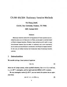
Numerical Integration of Experimental Data Sets For the first part of this project, we suppose that we are presented with the following experimental data on the heat capacity at constant pressure CP of solid lead at various temperatures up to and including 298 K (Table 1-2). We shall assume that CP ¼ 0 at T ¼ 0 K. We wish to obtain the absolute entropy of solid lead at 298 K. Each entry in Table 1-2 leads to a value of CP =T. The

25

ITERATIVE METHODS Table 1-2

Experimental Heat Capacities at Constant Pressure for Lead

T, K CP ; J K1 mol1

0 0 100 24.5

5 0.305 150 25.4

10 2.80 200 25.8

15 7.00 250 26.2

20 10.8 298 26.5

25 30 14.1 16.5

50 21.4

70 23.3

experimental data set can be entered into a Simpson’s rule integration program in the form of a DATA statement consisting of 14 number pairs, T first and CP =T second, in each pair. Note that spaces are not used in the data statement. There must be an even number of data pairs for Simpson’s rule integration because the subintervals are chosen in pairs. A Shortcut. The spreadsheet Excel (Appendix A) is available on many microcomputer systems. It is designed for business applications, not science, but it can be useful for handling large data sets. In this problem, we have a set of 14 CP values at corresponding T values and we would like to enter CP =T and T values into the program. Carrying out the repeated divisions by hand calculator is not very timeconsuming or error-prone for this small problem, but it would be in a research project generating hundreds of data points. Once entered into a spreadsheet, data can be manipulated column at a time. For example, let us take the ‘‘top cells’’ in Table 1-3 as cells A3 and B3 (columns A and B, line 3 in Table 1-3) containing 5 and 0.305 to avoid dividing 0 by 0. Using the easycalc option of the tools menu in Excel, divide the contents of B3 by A3 and place the results in cell C3. Now select C3 and the remaining 12 unfilled cells in the column, C3 to C15, and fill down using the mouse. The results of the calculation of CP =T appear for all remaining cells in the C column. Table 1-3

Excel Output for Entropy Calculations

T

CP

A1 0 5 10 15 20 25 30 50 70 100 150 200 250 298

B1 0 0.305 2.8 7 10.8 14.1 16.5 21.4 23.3 24.5 25.4 25.8 26.2 26.5

CP =T

0.061 0.28 0.46667 0.54 0.564 0.55 0.428 0.33286 0.245 0.16933 0.129 0.1048 0.08893

26

COMPUTATIONAL CHEMISTRY USING THE PC

Note that different spreadsheets and different versions of the same spreadsheet vary in the details of the calculation but that the basic idea for all is to carry out the calculation for the top cell and ‘‘fill in’’ the remaining cells in the same column with the mouse—a very convenient technique for simple calculations on large data sets. Consult the Help section of your spreadsheet for specific details. Program Program QENTROPY DIM X(100), Y(100) DATA 0,0,5,.061,10,.28,15,.4666,20,.54,25,.564,30,.55,50, .428, 70,.333,100,.245 DATA 150,.169,200,.129,250,.105,298,.089 N ¼ 14 0 FOR I ¼ 1 TO N: READ X(I), Y(I) this module reads the data set PRINT X(I), Y(I) NEXT I 0 FOR I ¼ 0 TO N  2 STEP 2 this module calculates the 0 S ¼ S þ (X(I þ 1)  X(I)) * (Y(I)) area of the rectangular S ¼ S þ (X(I þ 2)  X(I þ 1)) * Y(I þ 2) 0 blocks NEXT I 0 FOR I ¼ 0 TO N  2 STEP 2 this module calculates the area under 0 S ¼ S þ (X(I þ 1)  X(I)) * the parabolas 1, 4 in Fig. 1-3. (Y(I þ 1)  Y(I)) *.6667 S ¼ S þ (X(I þ 2)  X(I þ 1)) * (Y(I þ 1)  Y(I þ 2)) *.6667 NEXT I: PRINT PRINT ‘‘THE ENTROPY (CHANGE) IS:’’: PRINT S: END

The DIM statement in Program QENTROPY sets aside 100 memory locations for the experimental data points. It is necessary for any data set having more than 12 data pairs. What is the entropy of Pb at 100 and 200 K? Make a rough sketch of the curve of Cp vs. T for lead. Sketch the curve of Cp =T vs. T for lead. Sigmaplot and Tablecurve Jandel Scientific produces two programs that have many features useful in data processing. Both are rather complicated, intended for professional rather than student use, consequently some learning time must be invested to become proficient. This time is amply repaid later and the learning curve is not steep, so one can put these programs to practical use on relatively simple problems while learning how to handle more difficult ones. We shall give two examples here: curve plotting using SigmaPlot and curve fitting with numerical integration using TableCurve. On entering SigmaPlot (we use version 5.0), one is presented with a data table that is essentially a spreadsheet. Enter T as the independent or x-variable into the first column of the SigmaPlot data table and CP =T as the dependent or yvariable into the second column. The SigmaPlot data table should resemble columns 1 and 3 of Table 1-3. Rounding to three significant figures is permissible.

27

ITERATIVE METHODS 0.6

CP/T, J K–1 mol–1

0.5 0.4 0.3 0.2 0.1 0.0 0

50

100

Figure 1-8

150 T, K

200

250

300

CP =T vs. T for Lead.

After the data set has been entered and saved, one has several plotting options represented by icons in square boxes at the left of the data table. Click on the icon with a single zig-zag line to select a single plot on rectangular coordinates. After selection of the single plot option, one is presented with several suboptions. Select the option represented by the wavy line for a spline fit (similar to Simpson’s rule) to give a single continuous curve through the points. After selection of the spline fit, one is presented with a ‘‘plotting wizard’’ that asks if you want an x-y plot. Click yes. Now specify the x variable as column 1 and the y variable as column 2. The wizard will present you with the option Finish. Click on Finish to obtain a plot that is in all essential respects Fig. 1-8 except for some cosmetic changes that you can make according to the instructions in the SigmaPlot manual or the Help file. Different systems may require different protocols to obtain one of many possible graphs, and several protocols in one system often achieve the same result. At entry level, all this may seem a bit bewildering, but to anyone who has struggled with mechanical drawing tools to make a simple line drawing like Fig. 1-8, SigmaPlot seems a miracle. To anyone who has carried out curve-fitting calculations with a mechanical calculator (yes, they once existed) TableCurve (Appendix A) is equally miraculous. TableCurve fits dozens, hundreds, or thousands of equations to a set of experimental data points and ranks them according to how well they fit the points, enabling the researcher to select from among them. Many will fit poorly, but usually several fit well. We shall find the equation that best fits the points in columns 1 and 3 of Table 1-3 with TableCurve. On opening TableCurve, one is presented with a blank desktop with several commands at the top. The command to enter data is not Enter but Edit. Two formats are available, the TableCurve editor and the ASCII editor. The TableCurve format is probably a little simpler than the ASCII format, but they are both fairly self-evident and either should yield a data file resembling the data

28

COMPUTATIONAL CHEMISTRY USING THE PC

file for SigmaPlot. Each x-variable should be entered as an entry in the first column, followed by the y-variable as an entry in the second column. The statistical weight of each data point is 1, which is automatically entered in the TableCurve format. Click on Process ) Fit all equations and wait a moment while the curve fitting takes place. The formula of the best fit will appear with a graph showing the curve of the equation and the data points for comparison. In this case, the fit of the first ranked equation is very good. The first ranked equation turns out to be a quotient of polynomials y0:5 ¼ ða þ cx þ ex2 Þ=ð1 þ bx þ dx2 þ fx3 Þ

ð1-36aÞ

that is, Cp ða þ cT þ eT 2 Þ2 ¼ T ð1 þ bT þ dT 2 þ f T 3 Þ2

ð1-36bÞ

where constants a through f are empirical fitting constants given by the program. Equations fitting the curve with a lower ranking according to closeness of fit are also given. Along with the curve fitting process, TableCurve also calculates the area under the curve. According to the previous discussion, this is the entropy of the test substance, lead. To find the integral, click on the numeric at the left of the desktop and find 65.06 as the area under the curve over the range of x. The literature value depends slightly on the source; one value (CRC Handbook of Chemistry and Physics) is 64.8 J K1 mol1 . Mathcad Before posing the problem for this computer project, we shall introduce another very useful piece of microcomputer software by repeating the integration of Eq. (1-36a) with Mathcad (Appendix A). Like other software of this kind, there is a short learning process before mathcad can be used with ease. Once one has entered the equation of interest, mathcad solves it with a click on the ¼ sign. In the present example, the constants of (Eq. 1-36a) are entered followed by the desired integral a :¼ 0:013003 b :¼ 0:017052 c :¼ 0:068394 d :¼ 0:002334 f :¼ 0:000002912 ð 298 ða þ c  x þ e  x2 Þ2 dx ¼ 65:061 2 0 ð1 þ b  x þ d  x2 þ f  x3 Þ

e :¼ 0:000745

Note that the constants must be defined equal to their numerical values (defined ¼ is ; on the keyboard). These definitions must be above the integral you wish to solve. Mathcad operates top down. Mathcad produces the same value for the integral that we obtained from TableCurve. This calculation is redundant with the calculations already performed in this section to introduce new software by solving a problem for which we already know the answer.

ITERATIVE METHODS Table 1-4

29

Experimental Heat Capacities at Constant Pressure for an Unknown Metal

0,0,5,0.24,10,0.64,15,1.36,20,2.31,25,3.14,30,4.48,50,9.64,70,15.7,100,20.1,150,22.0, 200,23.4,250,24.3,298,25.5

The Problem (at last). A lustrous metal has the heat capacities as a function of temperature shown in Table 1-4 where the integers are temperatures and the floating point numbers (numbers with decimal points) are heat capacities. Print the curve of CP vs. T and CP =T vs. T and determine the entropy of the metal at 298 K assuming no phase changes over the interval [0, 298]. Use as many of the methods described above as feasible. If you do not have a plotting program, draw the curves by hand. Scan a table of standard entropy values and decide what the metal might be. PROBLEMS 1. Show that the area under a parabolic arc similar to Fig. 1-3 but that is concave upward is 13 wð f ðxi Þ þ 4f ðxiþ1 Þ þ f ðxiþ2 ÞÞ. 2. Compute the probability of finding a randomly selected experimental measurement between the limits of 0.5 standard deviations from the mean. 3. Given experimental measurements with m ¼ 123:4 and s ¼ 12:9, draw the entire probability distribution curve for the population of all experimental measurements in the class studied. 4. Write a program in BASIC to generate the area under the normal curve over the interval [0, 4] at intervals of 0.01z. 5. The program in Problem 4 gives final values for the integral under the normal curve that are obviously too large. The last entry is 0.5002, whereas, from the nature of the problem, we know that the integral cannot exceed 0.5000. Suggest a reason for this. 6. If Eq. (1-22) is normalized to 1.0, then ðb 2 f ðzÞ ¼ ez =2 dz a

pffiffiffiffiffiffi should be 2p for [1; 1]. Find out if this is true by numerical integration using limits on the integral that are wide enough that the area under the curve doesn’t change by more than a part per thousand or so for a small change in the limits of integration. 7. (a) Is the atomic wave function 1  ¼ pffiffiffi er p normalized to 1?

30

COMPUTATIONAL CHEMISTRY USING THE PC

(b) The probability that the electron in the H atom will be found at a radial distance r from the nucleus is ðr pðrÞ ¼ 4r 2 e2r dr 0

where r is measured in units of bohr (1 bohr ¼ 52.92 pm). What is the probability that the electron will be found within 2 bohr radii? (c) At approximately what radial distance is the probability of finding the H atom electron less than 1%? 8. What is the probability of finding an electron between 0.6 and 1.2 Bohr radii of the nucleus. Assume the electron to be in the 1s orbital of hydrogen. 9. The 2s orbital of hydrogen can be written  ¼ ð2  rÞer Plot this orbital with appropriate scale factors to determine the behavior of  in rectangular coordinates. Describe its behavior in spherical polar coordinates. 10. Plot the probability density obtained from  in Problem 9 as a function of r, that is, simply square the function above with an appropriate scale factor as determined by trial and error. Comment on the relationship between your plot and the shell structure of the atom. 11. Sketch the probability of finding an electron in the 2s orbital of hydrogen at distance r from a hydrogen nucleus as a function of r as a contour map with heavy lines at high probability and light lines at low probability. How does this distribution differ from the 1s orbital? 12. Draw the curve of CP vs. T and CP =T vs. T from the following heat capacity data for solid chlorine and determine the absolute entropy of solid chlorine at 70.0 K T

5

10

15

20

25

30

35

40

CP

0.14

1.10

3.72

7.74 12.09 16.69 20.79 23.97

50

60

70

29.25 33.47 36.32

13. Which of the following two integrals is wrong? ð1 1: 2:

1 2 2a ð01 1 2 x3 eax dx ¼ 2a 1 2

x3 eax dx ¼

14. A function for which f ðxÞ ¼ f ðxÞ over a specific intereval is called an odd function over that interval. If f ðxÞ ¼ f ðxÞ, the function is even. For example, y ¼ x, is an odd function over ½2; 2. The interval ½2; 2 is symmetrical about x ¼ 0. Write some odd functions. Write some even functions. Find a general rule for the integrals of odd functions over a symmetrical interval. Find a general rule for the integral of the product of an odd function and an even function over an interval that is symmetrical for both.