quantities. Based on this procedure, we also developed a deci- sion support
system (DSS) and implemented it for 600 of the most expensive Jeppesen charts.
Jeppesen Uses a Dynamic-Programming-Based DSS to Manage Inventory Elena Katok
[email protected]
Andrew Lathrop
[email protected]
William Tarantino
[email protected]
Susan H. Xu
[email protected]
Department of Management Science and Information Systems, Penn State University University Park, Pennsylvania 16802 Accenture Capability Modeling and Simulation 161 North Clark Street, Chicago, Illinois 60601 Center for Army Analysis 6001 Goethals Road, Fort Belvoir, Virginia 22060 Department of Management Science and Information Systems, Penn State University
We developed a system for managing inventory at Jeppesen Sanderson, Inc., a major provider of aviation-information products. The system determines order quantities for charts used in flight manuals. These charts contain essential safety information that changes frequently, making standard methods for inventory management ineffective. We formulated the problem as a dynamic programming model and developed a simple heuristic-solution procedure for determining order quantities. Based on this procedure, we also developed a decision support system (DSS) and implemented it for 600 of the most expensive Jeppesen charts. The system has been in use since August 1998, generating actual annual cost reductions of over $800,000.
J
eppesen Sanderson, Inc. (Jeppesen), in business since 1934, is the largest provider of aviation-information products in the world. Although Jeppesen manufactures many products, including flight simulators, aircraft maintenance manuals, and training videos, its most important product line consists of flight manuals. These
manuals, used by the majority of pilots flying today, are composed of charts (or maps), and Jeppesen manufactures, distributes, and maintains inventory of over 100,000 distinct charts used in over 2,000 different flight manuals. Jeppesen’s customers include most major airlines, such as United, US Airways, American, Delta,
Copyright 䉷 2001 INFORMS 0092-2102/01/3106/0054/$05.00 1526–551X electronic ISSN This paper was refereed.
DYNAMIC PROGRAMMING—APPLICATIONS INVENTORY/PRODUCTION—PERISHABLE/AGING ITEMS
INTERFACES 31: 6 November–December 2001 (pp. 54–65)
JEPPESEN Northwest, and Lufthansa; delivery services, such as Federal Express and UPS; and numerous corporate and private pilots. With the recent surge in information and media technology making an increase in competition imminent, Jeppesen, like many other firms, has been forced to cut costs while simultaneously improving customer service. Katok, Tarantino, and Tiedeman [2001] describe how Jeppesen uses operations research in its production planning. Jeppesen charts cover nearly the entire world. Flight manuals that include charts for particular geographic areas are called coverages. A given chart can be included in several different manuals. Coverages are composed of different types of charts that vary in size and color and contain different information. Small black and white charts (Figure 1) are manufactured in-house and are fairly inexpensive. Larger multicolor charts, however, are typically printed by outside vendors and are much more expensive. Inventory control at Jeppesen is complex because many charts must be revised often to keep
coverages current. Jeppesen manufactures charts to maintain stock levels and stores them in a large warehouse full of pigeonholes. The Jeppesen stock crew continuously maintains the pigeonholes, because, when a chart is revised, the existing inventory of that chart is scrapped. The crew then refills the pigeonholes with the updated versions. The process consumes production resources and can be expensive, depending on the efficiency of inventory policies. The Jeppesen problem belongs to the class of inventory problems with random lifetime, because once a chart is issued, it is generally not known when some information on it will change, so the chart’s life span is unknown. The two related problems discussed in the inventory-management literature deal with obsolete and perishable inventory. Barankin and Denny [1965] were the first to define the obsoleteinventory problem and to numerically compare systems with and without obsolescence. They defined obsolescence to mean that “the item in question is no longer to be used and the stock on hand is to be dis-
Figure 1: The majority of Jeppesen charts are 51⁄2ⴖ ⴒ 81⁄2ⴖ black and white sheets. These charts are printed in-house and are fairly inexpensive. Some charts, however, are large and multicolored. They are often outsourced and are more expensive.
November–December 2001
55
KATOK, LATHROP, TARANTINO, XU posed of.” Pierskalla [1969] further examined theoretical properties of the obsolescence model with deterministic demand when both holding and shortage costs are continuously differentiable convex functions, and he showed that when the probability of obsolescence is high it has a significant impact on the optimal policy. Nahmias [1977] assumed that both demands and lifetimes are stochastic and the ordering cost is proportional to the number of units ordered; he derived an explicit analytical expression for expected outdating, as well as two approximations. Rosenfeld [1989] further considered the problem with stochastic demand and probability of obsolescence when obsolete inventory has salvage value. Finkin [1989] suggested ways to manage obsolete inventory in practice. Perishability is slightly different from obsolescence and is relevant for products that are reordered regularly and became unfit for use after some time (which may or may not be known in advance). Perishable-inventory problems are common in the food and the health-care industries. An often-cited example is a blood bank’s inventory problem [Elston 1970; Jennings 1973; and Prastacos 1984], where the law mandating the useful lifetime of blood, because of its perishable nature, has a major impact on optimal inventory policies. In situations that blood banks and food producers encounter, the product degrades over time or has a fixed life and therefore any inventory-management system must track different-aged inventory. Researchers have analyzed the theoretical aspects of this class of problems. Nahmias and Pierskalla [1973] studied the perishable-
inventory model where product life span is known to be two periods, and Fries [1975] and Nahmias [1975] extended the model to the case of three or more periods. In these models, they assumed that the ordering cost is proportional to the number of units ordered. Nahmias [1978] relaxed this assumption to include fixed ordering cost, but with deterministic life spans. The Nahmias [1977] model does not allow fixed order costs, and we are unaware of any analytical models or applications combining uncertain life spans, stochastic demands, and fixed ordering costs, which is the situation Jeppesen faces. Fortunately, Jeppesen’s problem has several special features that facilitate the development of a computationally efficient approximatesolution algorithm. One factor that adds complexity to the perishable-inventory problem is that items of different ages will become outdated at different times, so the model must keep track of the different-aged inventory. In that sense, Jeppesen’s problem is more one of obsolescence and does not include this complication. When information on a chart changes and a new chart is issued, the entire inventory of the old chart is out
INTERFACES 31:6
56
Jeppesen charts cover nearly the entire world. of date, regardless of how long ago the individual charts were printed. In addition, the revision process for charts has a special feature. Revision dates on most charts fall into a distinct eight-week cycle. For some types of changes, revised charts must be issued as soon as information is
JEPPESEN received. But for many other changes, Jeppesen has an option of waiting several weeks, usually until the beginning of the next cycle, before reissuing. At Jeppesen, when a chart is revised, four demand components determine the quantity printed: (1) The actual subscription quantity, the number of customers who subscribe to manuals that contain the chart; (2) The additional production requirements, the charts mailed to customers or otherwise consumed during the revision process, beyond the subscription quantity; (3) The scrap allowance, the amount printed above the subscription quantity to replace the number of charts that will get damaged during the assembly process; and (4) The bin-stock quantity, the number printed for filling future order demand, which is often stationary during the lifetime of a chart. We focused on computing bin-stock quantities. The first three demand quantities are deterministic and occur only at the revision time. They are added to the binstock quantity for a new chart to determine the total quantity to be printed. Prior to implementing our work, Jeppesen determined the scrap and bin-stock quantities using a set of ad hoc rules that had evolved over many years and consistently overestimated print quantities. We observed nine pallets of charts costing over $15,000 being scrapped at the end of an eight-week cycle shortly before we began this study. Subsequently, a few weeks before Jeppesen started using our model, we observed 20 pallets being discarded. In 1998, Jeppesen’s inventory-management
system was part of the mainframe-based, so-called legacy system. The legacy systems do not include a relational database and can be controlled only through custom Cobol code. This makes them very difficult to customize. In 1999, Jeppesen completed a migration to an Oracle-based system, and our decision support system (DSS) is currently linked directly to Oracle. Prior to 1998, scrap and bin-stock quantities at Jeppesen had become inflated primarily for two reasons. First, production managers in different areas manually adjusted the scrap-allowance factors for charts in the legacy system. Unfortunately, since the legacy system was difficult to customize, changes in the scrap allowance affected all chart quantities regardless of chart type, greatly increasing waste. During the course of this project, we observed an increase in the quantity of charts scrapped because one manager felt that scrap quantities for charts printed inhouse were insufficient for his area. This adjustment, however, also affected outsourced charts that never even passed
November–December 2001
57
No one was aware of the scrap except the forklift driver. through this manager’s area. The impact on waste was considerable. Our DSS adds a scrap allowance of 10 charts for each coverage that includes the chart. This amount can be customized easily, but in the two years the system has been in use it has not been changed. Second, charts were ordered when revised or when the stock ran out before the next revision; reordering existing versions
KATOK, LATHROP, TARANTINO, XU of these charts required additional work and represented a visible expense. Frequent reorders attracted managers’ attention, but as long as an order met demand until the next revision, no one was aware of the scrap except the forklift driver who removed it every eight weeks: the classic victimless inventory crime. We developed a DSS for computing order policies for about 600 of Jeppesen’s most expensive outsourced charts. We based it on an approximate solution to a dynamic programming problem that considers charts’ revision history (the probability of obsolescence), stochastic weekly demand, and fixed order costs. Our system allowed Jeppesen’s planners to take the ordering of outsourced charts outside the legacy system, thus improving managerial control, and this saved about $800,000 per year. The Dynamic Programming Formulation We modeled the problem as a periodicreview inventory system with a random duration R, where R is the lifetime of a given chart. The history of time-betweenrevisions R for an outsourced chart was available to us, and we used the data to determine the empirical distributions of R. For simplicity, we assumed that the lifetimes of different charts are independent. Random lifetime R can assume a value kt, t ⳱ 1, 2, . . . , b, where k is a given integer representing the length of the revision cycle, and t denotes the cycle index with an upper bound b. In other words, the end of the chart life can occur only at the end of the ktth period, t ⳱ 1, . . . , b. In the case of Jeppesen, most charts we considered are revised on an eight-week cycle and last no more than six cycles, so k ⳱ 8, b ⳱ 6, and
a chart can be revised 8, 16, . . . , 48 weeks after initial printing. Jeppesen’s sales data show that demand for charts during their lifetimes is random but stable. Therefore, we modeled the weekly demand for a chart in week i as a random variable Di, where Di, i ⳱ 1, 2, . . . , are independent and identically distributed (iid) random variables having generic representation D. Again, we obtained the empirical distribution of D from the historical data. Printing outsourced charts has two costs. Before a chart can be printed (regardless of whether it has just been revised or is being reprinted) a plate must be created, with one or more negatives of the chart’s image burned onto this plate. Creating plates for offset printing is a time-consuming manual process, which we modeled by the fixed cost A that Jeppesen incurs whenever it places an order. After a plate is created, the rest of the printing cost is modeled by c, the unit variable production cost. Let y be the order quantity. The procurement function c(y) is given by
INTERFACES 31:6
58
c(y) ⳱
冦0A Ⳮ cy
when y ⱖ 0, when y ⳱ 0.
For simplicity, we assumed that orders can be filled instantaneously. In practice, vendors are responsive, and lead times for outsourced charts are typically under a week. At Jeppesen, the inventory-holding cost is considered sunk, so we let it equal zero. We assumed that the firm must reorder if inventory on hand is less than or equal to zero. As such, A can be regarded as the penalty cost of running short, and we do not assume a variable shortage cost.
JEPPESEN We formulated the Jeppesen problem as a dynamic programming (DP) problem. We defined the stage of the DP model, denoted by n, as the age of a chart, that is, the number of periods since the current revision was issued. We say that the process is in period n, n ⳱ kt Ⳮ i, t ⳱ 0, 1, . . . , b ⳮ1, and i ⳱ 1, . . . , k, if the current revision has age n. The state of the system in a period, denoted by x, is the starting inventory in that period. Our objective was to find the optimal ordering policy that would minimize the expected total procurement cost incurred during the lifetime of a chart. We let Vn(x) be the minimum expected procurement costs of a chart from period (age) n to the end of its life, given that the initial inventory at the beginning of period n is x. V1(0) represents the minimum expected total cost incurred during the lifetime of a chart. We called a period interior if the chart cannot be revised at the end of that period. An interior period has a time index n ⳱ kt Ⳮ i, i ⳱ 1, 2, . . . , k ⳮ 1, t ⳱ 0, 1, 2, . . . , b ⳮ 1. We called a period boundary if the chart’s life might end at the end of that period. In other words, a boundary period is the last period in a cycle and hence has a time index k(t Ⳮ 1), t ⳱ 0, 1, . . . , b ⳮ 1. In the case of Jeppesen, boundary periods are 8, 16, 24, 32, 40, and 48, and all other periods are interior (1, 2, . . . , 7, 9. . . , 15, 17. . . , 23, and so on). We denoted the remaining life of a chart, with age kt, by Rkt ⳱ R ⳮ kt | R ⬎ kt, t ⳱ 1, 2, . . . , b ⳮ 1.
ing life of t⬘ cycles, is given by P(Rkt ⳱ kt⬘) ⳱ P(R ⳱ k(t Ⳮ t⬘) | R ⬎ kt), t ⳱ 1, 2, . . . , b ⳮ 1, t⬘ ⳱ 1, 2, . . . , b ⳮ t.
The above conditional probabilities can be determined based on the empirical distribution of R. Next, we derived the optimality equations for interior and boundary periods. The DP recursion corresponding to an interior period is VktⳭi(x) ⳱
min yⳭx⬎0,yⱖ0
{c(y) Ⳮ EVktⳭiⳭ1(x Ⳮ y ⳮ D)},
i ⳱ 1, 2, . . . , k ⳮ 1, t ⳱ 0, 1, . . . , b ⳮ 1.
(1)
Here, c( y) is the procurement cost incurred in interior period kt Ⳮ i if Jeppesen orders quantity y, and EVtkⳭiⳭ1(x Ⳮ y ⳮ D) is the expected cost from kt Ⳮ i Ⳮ 1 onward, assuming it acts optimally in the future. The problem in period kt Ⳮ i, then, is to choose y that minimizes the sum of the present and future procurement costs. The constraints on the order quantity y in (1) mean that the firm never scraps onhand inventory in the middle of a cycle, and when on-hand inventory falls to or below zero, it must place an order. Let [a]Ⳮ ⳱ max {0,a}. The DP recursion corresponding to a boundary period (the last period of a cycle) is Vk(tⳭ1) (x) ⳱
冦
min yⳭx⬎0,yⱖ0
冧
c(y) Ⳮ P(Rkt ⬎ k) EVk(tⳭ1)Ⳮ1 (x Ⳮ y ⳮ D) Ⳮ P(Rkt ⳱ k) , (AP(D ⬎ x Ⳮ y) Ⳮ cE[D ⳮ x ⳮ y]Ⳮ)
Then the conditional probability that the current revision, with age kt, has a remain-
(2) t ⳱ 0, 1, . . . , b ⳮ 1. The above optimality equation is understood as follows: c(y) is the procurement
November–December 2001
59
KATOK, LATHROP, TARANTINO, XU cost incurred in the boundary period k(t Ⳮ 1). The future costs depend on whether the chart would be revised at the end of the period. With probability P(Rkt ⬎ k), the chart with age kt will survive at least another cycle, and the process evolves to the next interior period k(t Ⳮ 1) Ⳮ 1 with the minimum expected cost EVk(tⳭ1)Ⳮ1 (x Ⳮ y ⳮ D). With probability P(Rkt ⳱ k), the chart ends its life at the end of the (t Ⳮ 1)st cycle, in which case the system incurs reorder cost A with probability P(D ⬎ x Ⳮ y) and production cost cE[D ⳮ x ⳮ y]Ⳮ. When t ⳱ b ⳮ 1 in (2), Vkb(x) gives the boundary condition of the DP recursion, with P(Rk(bⳮ1) ⳱ k) ⳱ 1. Theoretically, one can solve Equations (1) and (2) using a standard DP computational technique, such as value iterations. However, such an approach is impracti-
cal for the Jeppesen problem because of its large size. A typical Jeppesen chart lasts up to five or six cycles, with each cycle consisting of eight weeks, meaning that the planning horizon is 40 or 48 weeks long. The weekly demand D can usually be approximated by a normal random variable D ⬃ N (d, r2), where d can take a value between 10 and 700, resulting in a DP problem with an extremely large state space. In addition, because of the positive setup cost, Vn(x) is not convex and may have multiple local minima. To overcome computational complexity and facilitate implementation, we developed and implemented a simple heuristic method.
A Simple Heuristic Solution Procedure Our heuristic method consists of two steps: In the first step, we determine the order-up-to cycle under the simplifying assumption that the weekly demand is deterministic and equals its mean, d ⳱ E(D). In the second step, we determine the order quantity that equals the mean demand until the next order plus safety stock. If weekly demand is deterministic, d ⳱ E[D], then our model becomes a variant of Wagner and Whitin’s [1958] dynamic lotsizing problem with a random lifetime that may end at the end of a boundary period k(t Ⳮ 1), t ⳱ 0, 1, . . . , b ⳮ 1. The standard Wagner-Whitin algorithm has the following properties: it places an order only when starting inventory is zero, and its order size must cover demand for an integer number of periods. Our simplified problem has properties that resemble those of the Wagner-Whitin dynamic lotsizing problem, as stated in the following theorem: Let the demand in each period be deterministic, d ⳱ E(D). (1) One does not place an order in a period, given that the chart has not become obsolete, if the stock on hand is sufficient to meet the demand to the end of its cycle. (2) When ordering, one brings stocks to such a level that they exactly satisfy the demand up to the end of a cycle. (We give the proof in the Appendix.) This result implies that if the demand in each period is deterministic, d ⳱ E(D), then an order is placed only at the beginning of a cycle and the order quantity must cover demand for an integer number of future cycles. So, at the beginning of the tth cycle, we seek to find the optimal
INTERFACES 31:6
60
The DSS virtually eliminated reorders.
JEPPESEN order-up-to cycle l*, t t ⳱ 0, 1, 2, . . . , b ⳮ 1. Let L(t⬘) be the total ordering and production cost for demand in t⬘ cycles. Then
When we implemented this heuristic at Jeppesen, we chose a very conservative safety stock factor ␣ ⳱ 3.6, or 3.6 standard deviations of demand during a reorder cycle. We based this choice on the following considerations: —Since the ordering cost is very high relative to production cost (typically ordering cost is about $1,200; and variable production cost is 20 cents per chart), we wish to
virtually eliminate the possibility of the actual demand during (l *t ⳮ t) cycles exceeding the order quantity ¢ yt, t ⳱ 0, 1, . . . , b ⳮ 1. We chose the factor of 3.6 to approximately balance the impact of shortage and overage. In the case of a reorder, the plating cost overwhelms the printing cost, so the ratio between the typical printing cost and the typical plating cost is 0.2/1,200 ⳱ 0.000167, and the factor of about 3.6 (actually, 3.58) gives the probability of stock out 0.000167. Because the plating cost is fixed, this is only an approximation. —By placing an order only at the beginning of a cycle, we were able to effectively prolong the time between reviews (from a week to eight weeks) and thus reduce the monitoring effort in inventory management. We based our cyclic review policy on maintaining very conservative safety stock, which makes the probability of shortage within a cycle approximately zero. This cyclic ordering schedule is also more convenient for the planners, since it saves time and reduces errors. —Although we do not discuss this benefit in this paper, the cyclic ordering pattern also enables Jeppesen to order more of its charts at one time, saving additional expense by plating smaller charts together, thus reducing plating costs. A fundamental insight was that a chart’s order quantity at the beginning of a cycle should be related to its remaining lifetime and the demand distribution. Before we implemented our work, order quantities were not a function of the distributions of weekly demand and remaining lifetime but were hard-coded into the legacy system as a function of the current subscrip-
November–December 2001
61
L(t⬘) ⳱ A Ⳮ ckt⬘d, t⬘ ⳱ 1, 2, . . . , b ⳮ 1.
(3)
¢ t ⬅ VktⳭ1 (0). The optiFor simplicity, let V mality equation at the beginning of the tth cycle becomes ¢ t ⳱ min {L(t⬘) Ⳮ P(Rkt ⬎ kt⬘)V ¢ tⳭt⬘}, V 0⬍t⬘ⱕbⳮt
t ⳱ 0, 1, 2, . . . , b ⳮ 1,
(4)
with the boundary condition ¢ bⳮ1 ⳱ L(1) ⳱ A Ⳮ ckd. V
(5)
The cost function (4) can be calculated recursively starting from the cost function of the last cycle, using (5). After using (3) through (5) to determine the optimal order-up-to-cycle l *, t t ⳱ 0, 1, . . . , b ⳮ 1, we determine the approximate optimal order quantity ¢ yt ⬅ y*ktⳭ1, by adding a safety stock amount, ¢ st, to the average demand during cycles t and l *. t We get ¢t ⳱ (l *t ⳮ t)kd Ⳮ s¢t, y t ⳱ 0, 1, 2, . . . , b ⳮ 1, where ¢ st is determined by s¢t ⳱ ␣冪(l t* ⳮ t)kr2.
(6)
KATOK, LATHROP, TARANTINO, XU
Figure 2: In this overview of the DSS, the legacy system provides the bill of materials (BOM) for all coverages. The data module combines the BOM with new-orders history to compute average weekly demand for each chart. The forecast module allows the user to select parameters for the moving-average forecasting model and computes average weekly demand and the standard deviation of the weekly demand for charts in the system. The inventory module computes the optimal reorder cycle using the model we developed and combines it with specific chart information from the legacy system to come up with the final order quantity.
tion quantity. Since the legacy system has no view of either remaining life or demand distributions, the current subscription quantity was the best available proxy measure. The current subscription quantity is at best an indirect indicator of weekly demand and is no indicator at all of time between revisions. Therefore, the legacy order quantities did not generally provide a good solution to the problem. As one would expect, the simple heuristic solution performs well when demand variability is low (demands for most Jeppesen charts have low variances relative to their means). If demand is highly variable, then the heuristic method will generate a
large amount of safety stock, as can be seen from (6). Therefore, the heuristic method might perform rather poorly when demand has a low mean and a high variance, especially when production cost c is large relative to ordering cost A. In such a case, it might be beneficial to order more than once to keep safety stocks low. Katok and Xu [2000] have developed and compared several other heuristic methods that take demand variability into consideration. Currently, Jeppesen has implemented only the simple heuristic method described. DSS Implementation Details Figure 2 shows an overview of the DSS. Although the algorithm we use is compu-
INTERFACES 31:6
62
JEPPESEN
Figure 3: These are two typical distributions for time between revisions. Charts are never revised in less than eight weeks, and most charts do not last longer than 48 weeks. A typical time between revisions is 16, 24, or 32 weeks.
tationally simple, some of the data required considerable collection effort and statistical analysis. Specifically, deriving the revision history distribution and the distribution of weekly demand for each chart required a great deal of analysis. In fact, we quickly determined that deriving these distributions, and implementing and maintaining an inventory management system would not be cost effective for all charts. For these reasons, we limited our DSS to the more expensive outsourced charts. We collected revision data from 1990 to 1998 and developed empirical distributions for the time between revisions of all outsourced charts (Figure 3). These are two typical distributions for time between revisions: Charts are never revised in less than eight weeks, and most charts do not last longer than 48 weeks. A typical time between revisions is 16, 24, or 32 weeks. It was cumbersome to compute weekly demand distributions for individual charts, and Jeppesen’s legacy system did not support the automation of this procedure. Since the beginning of 1997, however, Jeppesen has managed new orders through a
Microsoft Access database, and we were able to estimate weekly demand distributions easily. We implemented the solution method using Microsoft Excel. The Excel spreadsheet yields the optimal reorder cycle. All chart-specific data are maintained in two Microsoft Access databases. To check the system’s robustness, we examined eight chart types from different geographical areas and computed the total annual cost as a function of the order period. The eight types differ in their demand distribution, the number of coverages in which the charts are used, and in the revision-history distribution. Nevertheless, we note a striking similarity in the shapes of the cost curves, showing that it is much more expensive to underorder than to overorder. This is not surprising, since the penalty for underordering is a high fixed order cost, while the penalty for overordering is a much lower variable cost. To make the model more robust to overordering, we included logical rules in the system that always err on ordering too much rather than too little. The purpose of these rules is to make the solution less
November–December 2001
63
KATOK, LATHROP, TARANTINO, XU sensitive to data errors. System Impact The implementation of the system proceeded in three stages: —Evaluation and development from January to August 1998; —The initial test from August to December 1998; —System enhancement from December 1998 to March 1999. In January 1998, we started investigating inventory-related issues at Jeppesen and noticed that it consistently overordered enroute charts, some by as much as 10,000 over its official legacy bin-stock quantities. The inventory manager lacked confidence in Jeppesen’s information system, and planners worried that they would run out of charts for the current revision. We checked the legacy subscription quantities and verified their accuracy. At that time, we discovered an additional requirement portion of demand. These additional requirements were not well understood at Jeppesen, but we were able to quantify them well enough to ascertain that the official Jeppesen print quantities were always sufficient for the current revision. Reassured, Jeppesen’s schedulers started ordering the exact quantities specified by the legacy system. In August 1998, we implemented the DSS for inventory management. Jeppesen’s schedulers immediately started using the system. The system records every order placed, including orders placed because of stock outs. It also calculates savings based on the difference between actual order quantities and the legacy system’s order quantities. Jeppesen managers worried that, since
our system generally prescribes lower order quantities, the cost of reorders due to stock outs would increase. To create a benchmark for this cost, we examined a year of invoices from June 1997 through June 1998. During that year, Jeppesen’s reorder costs for the enroute charts were
INTERFACES 31:6
64
Our system saved over $800,000 per year. over $250,000. With the new DSS, reorder costs from August 1998 through July 1999 were less than $23,000. The DSS virtually eliminated reorders. The reason for this dramatic decrease was that our system triggers a reorder when on-hand inventory drops to a very low level (less than one week’s demand). Since the system is very conservative in its order quantities, this virtually never happens. The old system triggered a reorder whenever inventory levels fell below bin-stock quantity. During the six-month period between June 1997 and December 1998 Jeppesen spent about $250,000 ordering charts above the official legacy order quantities. It halted this practice in January 1998, eliminating about $500,000 in annual costs. Finally, the DSS reported savings in variable costs between August 1998 and July 1999 of $120,000. Our system saved a total of over $800,000 per year. APPENDIX Proof (1) Suppose p* ⳱ {y*, n n ⳱ 1, 2, . . . , kb} is an optimal policy for ordering, where y*n is the stock on hand after ordering in period n, given that the chart has not become obsolete by n. Suppose that initial stock x in period n ⳱ kt Ⳮ i is sufficient to meet the remaining demand of the current cy-
JEPPESEN cle, that is, x ⱖ (k ⳮ i Ⳮ 1)d, but policy p* prescribes y*n ⬎ x. Let ¢ p be the policy that is the same as p* except that in following it one would not place an order in period kt Ⳮ i but would order the stock to level ( y*ktⳭi ⳮ x) Ⳮ y*k(tⳭ1)Ⳮ1 at the beginning of the next cycle (period k(t Ⳮ 1) Ⳮ 1) if the chart were not revised by then. If the chart were obsolete at the end of the current cycle, then following policy ¢ p would save a cost A Ⳮ c( y*ktⳭi ⳮ x). If the chart would not be revised in period k(t Ⳮ 1) Ⳮ 1 and following policy p* does not mean placing an order in that period, then the two policies would induce the same cost. If the chart would not be revised in period k(t Ⳮ 1) Ⳮ 1 and a planner following policy p* places an order in that period, then policy ¢ p would save an ordering cost A. (2) Suppose that in period n, n ⬍ kt, for some t, a planner following policy p* orders enough to cover demand to the end of period kt but not enough to cover demand to the end of period k(t Ⳮ 1); that is, y*n ⳱ (kt ⳮ n Ⳮ 1)d Ⳮ e, where 0 ⱕ e ⬍ kd. Note that, by (1), a planner following policy p* would not place an order during n Ⳮ 1, . . . , kt but would have to place an order in a period during kt Ⳮ 1, . . . , k(t Ⳮ 1) if the chart had not expired during period kt Ⳮ 1. Without loss of generality, let us assume that a planner following policy p* places an order in period kt Ⳮ 1. Consider another policy ¢ p that is the same as p* except that its order-up-to levels in periods n and kt Ⳮ 1 are y*n ⳮ e and y*ktⳭ1 Ⳮ e, respectively, provided that the chart had not become obsolete by period kt Ⳮ 1. If the chart became obsolete before period kt Ⳮ 1, following policy ¢ p would save production cost ce. Otherwise, the costs under the two policies would be the same. Hence e ⳱ 0 is an optimal policy. References Barankin, E. W. and Denny, J. 1965, “Examination of inventory model incorporating probabilities of obsolescence,” Logistics Review and
Military Logistics Journal, Vol. 1, No. 1, pp. 11–25. Elston, R. C. 1970, “Blood bank inventories,” CRC Critical Reviews in Clinical Laboratory Sciences, Vol. 1, No. 3 (July), pp. 527–545. Finkin, E F. 1989, “How to limit inventory expenses,” Journal of Business Strategy, Vol. 10, No. 1, pp. 50–53. Fries, Brant E. 1975, “Optimal ordering policy for a perishable commodity with fixed lifetime,” Operations Research, Vol. 23, No. 1, pp. 46–61. Jennings, J. 1973, “Blood bank inventory control,” Management Science, Vol. 19, No. 5, pp. 637–645. Katok, E.; Tarantino, W.; and Tiedeman, R. 2001, “Flexibility planning and technology management at Jeppesen Sanderson, Inc.,” Interfaces, Vol. 31, No. 1, pp. 7–29. Katok, E. and Xu, S. H. 2000, “Managing inventory with stochastic demand and product life-cycle length,” Working paper, Penn State University. Nahmias, Steven 1975, “Optimal ordering policies for perishable inventory—II,” Operations Research, Vol. 23, No. 4, pp. 735–749. Nahmias, S. 1977, “On ordering perishable inventory when both demand and lifetime are random,” Management Science, Vol. 24, No. 1, pp. 82–90. Nahmias, Steven 1978, “The fixed-charge perishable inventory problem,” Operations Research, Vol. 26, No. 3, pp. 464–481. Nahmias, Steven and Pierskalla, W. P. 1973, “Optimal ordering policies for a product that perishes in two periods subject to stochastic demand,” Naval Research Logistics Quarterly, Vol. 20, No. 2, pp. 207–229. Pierskalla, W. P. 1969, “An inventory problem with obsolescence,” Naval Research Logistics Quarterly, Vol. 5, No. 3, pp. 217–228. Prastacos, Gregory P. 1984, “Blood inventory management: An overview of theory and practice,” Management Science, Vol. 30, No. 7, pp. 777–800. Rosenfeld, Donald B. 1989, “Disposal of excess inventory,” Operations Research, Vol. 37, No. 3, pp. 404–409. Wagner, H. M. and Whitin, T. M. 1958, “Dynamic version of the economic lot size model,” Management Science, Vol. 5, No. 1, pp. 89–96.
November–December 2001
65