Journal of Computational and Applied Mathematics A variable ... - Core

Journal of Computational and Applied Mathematics 233 (2010) 2387–2394

Contents lists available at ScienceDirect

Journal of Computational and Applied Mathematics journal homepage: www.elsevier.com/locate/cam

A variable step implicit block multistep method for solving first-order ODEs S. Mehrkanoon ∗ , Z.A. Majid, M. Suleiman Department of Mathematics, Faculty of Science, University Putra Malaysia, 43400 UPM, Serdang, Selangor, Malaysia

article

info

Article history: Received 22 June 2009 Received in revised form 17 October 2009 MSC: 65L05 65L06 Keywords: Block method Variable step size Ordinary differential equations

abstract A new four-point implicit block multistep method is developed for solving systems of first-order ordinary differential equations with variable step size. The method computes the numerical solution at four equally spaced points simultaneously. The stability of the proposed method is investigated. The Gauss–Seidel approach is used for the implementation of the proposed method in the PE (CE )m mode. The method is presented in a simple form of Adams type and all coefficients are stored in the code in order to avoid the calculation of divided difference and integration coefficients. Numerical examples are given to illustrate the efficiency of the proposed method. © 2009 Elsevier B.V. All rights reserved.

1. Introduction In many fields of application in, e.g., science and engineering one can find equations of the form Y 0 = F ( x, Y )

Y (a) = Y0 ,

a≤x≤b

(1)

where a and b are finite and Y 0 = [y01 , y02 , . . . , y0n ]T , Y = [y1 , y2 , . . . , yn ]T and F = [f1 , f2 , . . . , fn ]T . Most of the existing methods for solving ODEs like that in (1) will only approximate the numerical solutions at one point, sequentially. Thus, developing faster methods which can give faster solutions to the problem are needed. Block methods for the numerical solution of first-order ODEs have been proposed by several authors, such as [1–4]. Among the earliest researchers investigating the block method, Houwen and Sommeijer [5] have developed block Runge–Kutta methods, Omar [6] introduced a block method based on Adams formulas for solving higher order ODEs and Majid [7] proposed a variable step size and order Adams type block method. The advantage of a block method is that in each application, the solution will be approximated at more than one point. The number of points depends on the structure of the block method. Therefore, applying these methods can give faster solutions to the problem and also can be managed to produce a desired accuracy. The authors in [8,9] have introduced a four-point diagonally and fully implicit block method in which at each application of the method, the solution will be approximated at four points simultaneously. The Jacobi iteration was used for the implementation of the methods in [8,9]. The Gauss–Seidel approach for the implementation of the two-point block one-step method was discussed in [10]. In this paper, the same approach will be considered for the four-point implicit block multistep method. The proposed block method will approximate the solutions at four points simultaneously in each step, using variable step size.

∗

Corresponding author. Tel.: +60 172063462; fax: +60 389437958. E-mail address: [email protected] (S. Mehrkanoon).

0377-0427/$ – see front matter © 2009 Elsevier B.V. All rights reserved. doi:10.1016/j.cam.2009.10.023

2388

S. Mehrkanoon et al. / Journal of Computational and Applied Mathematics 233 (2010) 2387–2394

Fig. 1. Four-point implicit block multistep method.

The method is derived by using the Lagrange interpolation polynomial and the closest point in the interval will be considered for obtaining the corrector and predictor formula. Therefore, the approximated values of yn+1 , yn+2 , yn+3 and yn+4 are obtained by integrating (1) over the intervals [xn , xn+1 ], [xn+1 , xn+2 ], [xn+2 , xn+3 ] and [xn+3 , xn+4 ] respectively. 2. Derivation of the four-point implicit block multistep method In Fig. 1, the solutions for yn+1 , yn+2 , yn+3 and yn+4 with step size h at the points xn+1 , xn+2 , xn+3 and xn+4 respectively are approximated simultaneously using five back values at the points xn , xn−1 , xn−2 , xn−3 and xn−4 of the previous four steps with step size rh. The set of points {xn−7 , . . . , xn } are used for deriving the predictor formula and the order is 1 less than the order of the corrector. The method will compute the solution at four points concurrently using four earlier steps. The interpolation points involved for obtaining the corrector formulas for yn+1 , yn+2 , yn+3 and yn+4 are {(xn−4 , fn−4 ), . . . , (xn+4 , fn+4 )}. The first point yn+1 is derived by integrating (1) as follows:

Z

xn+1

y0 dx =

Z

xn

xn+1

f (x, y) dx.

xn

Then y(xn+1 ) = y(xn ) +

xn+1

Z

f (x, y) dx.

(2)

xn

The function f (x, y) in (2) is approximated by the Lagrange polynomial which interpolates the set of points mentioned. Evaluating the integral using MATHEMATICA will give the formula for the first point in terms of r as follows. The first point: 17010r 3 + 13530r 2 + 4005r + 413

yn+1 = yn + h

+ +

34020r 3 + 23370r 2 + 5340r + 413 20160r 4 (r + 1)(r + 2)(2r + 1)(2r + 3)

fn−2 −

fn +

44352r 4 + 43050r 3 + 17220r 2 + 3165r + 220 20160(r + 1)(r + 2)(2r + 1)(3r + 2)

241920(r + 1)(r + 2)(r + 4)(3r + 4)

6480r 4 (r + 1)(3r + 1)(3r + 2)(3r + 4)

15120r 4 (r + 1)(r + 2)(r + 3)(r + 4)

725760r 4

19152r 4 + 17850r 3 + 6930r 2 + 1245r + 85

6480r 3 + 4920r 2 + 1335r + 118

136080r 3 + 63960r 2 + 12015r + 826

253008r 4 + 141750r 3 + 43050r 2 + 6675r + 413

× fn+1 − −

241920r 4 (r + 1)(2r + 1)(4r + 1)(4r + 3)

f n −4 −

fn−3

fn−1

325584r 4 + 394800r 3 + 190260r 2 + 41010r + 3275 15120(r + 1)(2r + 1)(3r + 1)(4r + 1) f n +2 +

7632r 4 + 7200r 3 + 2820r 2 + 510r + 35 6480(r + 1)(r + 3)(2r + 3)(4r + 3)

fn+3

f n +4 .

(3)

The approximate value for the second point, yn+2 , is derived by integrating (1) over the interval [xn+1 , xn+2 ]. Approximating f using the Lagrange polynomial and lastly evaluating the integral using MATHEMATICA, the formula for the second point in terms of r is obtained as follows. The second point:

yn+2 = yn+1 + h −

6930r 3 + 18810r 2 + 15525r + 3997

fn−4 +

2640r 3 + 6840r 2 + 5175r + 1142

(r + 1)(2r + 1)(4r + 1)(4r + 3) 6480r 4 (r + 1)(3r + 1)(3r + 2)(3r + 4) 13860r 3 + 32490r 2 + 20700r + 3997 55440r 3 + 88920r 2 + 46575r + 7994 − f n −2 + fn−1 4 20160r (r + 1)(r + 2)(2r + 1)(2r + 3) 15120r 4 (r + 1)(r + 2)(r + 3)(r + 4) 19152r 4 + 57750r 3 + 59850r 2 + 25875r + 3997 − fn 4 + +

241920r 4

725760r 174384r 4 + 478800r 3 + 454860r 2 + 181710r + 26165 15120(r + 1)(2r + 1)(3r + 1)(4r + 1) 76608r 4 + 261450r 3 + 306180r 2 + 149085r + 25820 20160(r + 1)(r + 2)(2r + 1)(3r + 2)

fn+1

f n +2

fn−3


− +

5328r 4 + 16800r 3 + 18180r 2 + 8190r + 1315 6480(r + 1)(r + 3)(2r + 3)(4r + 3)

2389

fn+3

11088r 4 + 34650r 3 + 37170r 2 + 16605r + 2645 241920(r + 1)(r + 2)(r + 4)(3r + 4)

f n +4 .

(4)

For deriving the approximate values for the third and fourth points yn+3 and yn+4 , the intervals [xn+2 , xn+3 ] and [xn+3 , xn+4 ] are used respectively and after evaluating the integral, the formulas for the third and fourth points are obtained as follows. The thirrd point: 6930r 3 + 32010r 2 + 44325r + 18893

yn+3 = yn+2 + h

+ + − + + −

fn−4 −

241920r 4 (r + 1)(2r + 1)(4r + 1)(4r + 3)

13860r 3 + 55290r 2 + 59100r + 18893 20160r 4 (r + 1)(r + 2)(2r + 1)(2r + 3)

fn−2 −

2640r 3 + 11640r 2 + 14775r + 5398 6480r 4 (r + 1)(3r + 1)(3r + 2)(3r + 4)

55440r 3 + 151320r 2 + 132975r + 37786 15120r 4 (r + 1)(r + 2)(r + 3)(r + 4)

fn−3

fn−1

11088r 4 + 57750r 3 + 101850r 2 + 73875r + 18893

fn 725760r 4 37296r 4 + 193200r 3 + 338940r 2 + 244590r + 62245 15120(r + 1)(2r + 1)(3r + 1)(4r + 1)

fn+1

76608r 4 + 376950r 3 + 629580r 2 + 433635r + 105620 20160(r + 1)(r + 2)(2r + 1)(3r + 2) 24912r 4 + 139200r 3 + 263220r 2 + 204510r + 55955 6480(r + 1)(r + 3)(2r + 3)(4r + 3)

fn+3

19152r 4 + 101850r 3 + 183330r 2 + 135645r + 35365 241920(r + 1)(r + 2)(r + 4)(3r + 4)

fn+2

fn+4 .

(5)

The fourth point:

yn+4 = yn+3 + h −

17010r 3 + 111210r 2 + 217125r + 129997 241920r 4 (r + 1)(2r + 1)(4r + 1)(4r + 3) 3

× fn−3 − × fn−1 − + − + +

fn−4 +

2

34020r + 192090r + 289500r + 129997

fn−2 +

6480r 3 + 40440r 2 + 72375r + 37142 6480r 4 (r + 1)(3r + 1)(3r + 2)(3r + 4)

136080r 3 + 525720r 2 + 651375r + 259994

(r + 1)(r + 2)(2r + 1)(2r + 3) 15120r 4 (r + 1)(r + 2)(r + 3)(r + 4) 19152r 4 + 141750r 3 + 353850r 2 + 361875r + 129997 20160r 4

725760r 4 4 3 53424r + 394800r + 984060r 2 + 1004910r + 360485 15120(r + 1)(2r + 1)(3r + 1)(4r + 1) 44352r 4 + 326550r 3 + 811020r 2 + 825315r + 295060 20160(r + 1)(r + 2)(2r + 1)(3r + 2) 46512r 4 + 331200r 3 + 796620r 2 + 786210r + 273005 6480(r + 1)(r + 3)(2r + 3)(4r + 3)

fn

fn+1

fn+2 fn+3

253008r 4 + 1966650r 3 + 5152770r 2 + 5527005r + 2080805 241920(r + 1)(r + 2)(r + 4)(3r + 4)

fn+4 .

(6)

During the implementation of the method, the choice for the next step size will be limited to half, double or the same as the current step size. If the approximated solution at step i has the desired accuracy therefore, the choice for the next step will be double or the same as the current step size which may be specified by the step size controller. Otherwise the step size becomes half. In the code developed, when the next step size is doubled, the ratio r is 0.5 and q can be 0.5 or 0.25, but if the next step size remains constant, r is 1 and q can be 1, 2 or 0.5. In the case of step size failure, r is 2 and q is 2. In order to reduce the computational cost, all the coefficients of the formula are stored in the code developed. In our code, an estimation of the local truncation error is obtained by comparing the derived corrector formula of order p at the fourth point, and the same corrector formula for that point of order p − 1. 3. Implementation of the four-point implicit block multistep method The method is implemented in PE (CE )m mode where P stands for an application of the predictor, E stands for an evaluation of the function f , and C stands for an application of the corrector. During the implementation, the iteration

2390


a

b

Im

c

Im 2

Im 0.10

0.3 0.2

1

0.05

0.1 Re

–0.6 –0.5 –0.4 –0.3 –0.2 –0.1 –0.1

–2.5

–2.0

–1.5

–1.0

Re

–0.5

–0.05

–1

–0.2

Re

–0.12 –0.10 –0.08 –0.06 –0.04 –0.02

–0.3

–0.10 –2

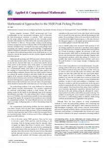
Fig. 2. Stability regions of the 4PG method for r = 1, 2 and 0.5.

involved the Gauss–Seidel approach. The iteration processes are as follows: n X

P : y0n+k = yn +

αj,k fj

j=n−7

E : f (xn+k , y0n+k ) for k = 1, 2, 3, 4 C : ym n+1 = yn +

n+4 X

βj,1 fj

j =n −4

E : f (xn+1 , ym n +1 ) m C : ym n+k = yn+k−1 +

n+4 X

βj,k fj

j =n −4

E : f (xn+k , ym n+k ) for k = 2, 3, 4; m = 1, 2, . . . until convergence. The estimation of the values of ym n+1 used the approach of Jacobi iteration, while for obtaining the approximate values 4 4 of {ym } at the points { x } respectively at the mth iteration, the Gauss–Seidel iteration is utilized. This strategy is n + k n+k k=2 k=2 called the half-Gauss–Seidel approach. 4. Absolute stability The absolute stability of the proposed method (4PG) when using a linear first-order test problem y0 = f = λy

(7)

is discussed. The stability region is plotted when the step size ratio is constant, doubled and halved for the method. The test Eq. (7) is substituted into the corrector formula of the method. Setting the determinant of the corrector formula written in matrix form to zero will give the stability polynomial. The stability polynomials of the proposed method are indicated by Pr (h, t ) for r = 1, 2 and 0.5 as follows: P1 (h, t ) =

11600004251h

4

266716800000

−

30875874257h 96018048000

2866557567341521h

4

3

+

1731045419h 1714608000

2819452741398091h

3

2

−

284231h 181440

+ 1 t8

3456684654973h

2

243847h

+ − − − 1 t7 + − 1106127912960000 1244393902080000 658409472000 48384 4 3 2 2576441875902911h 1525249994096917h 2655032011267h 119879h 6 + − + − − t 1548579078144000 622196951040000 658409472000 181440 4 3 2 285669233826133h 3967050582701h 7445161h + − − + t5 7742895390720000 1244393902080000 1714608000 4 3 4 1719659149h 424523h h t3 + t4 − =0 + 221225582592000

480090240000

266716800000


P 2 ( h, t ) =

4

176184892909h

2475465300000

−

44356877351h

3

+

99018612000

2467136772899h

4

1453443823h

2

−

1178793000

76252356690487h

3

481592h 280665

63034470887h

2

2391

+ 1 t8

7937527h

+ − − − − − 1 t7 3600676800000 63371911680000 25147584000 3548160 4 3 2 10352046479867h 12084391685411h 688130353721h 2702789h 6 + − − − − t 1013950586880000 289700167680000 9656672256000 57480192 4 3 2 86641867h 88272468283h 44583571h + + + t5 23044331520000 6489283756032000 3218890752000 ! 4 3 4 + P0.5 (h, t ) =

6684661h

162232093900800000 32240260037h

4

1237732650000

+

894947h

10815472926720000 3

−

22324404847h 99018612000

3820257223h

+

598878316837h

162232093900800000

2

4715172000

198156608h

77358290625

+

4193691525983h

6117376h

1719073125

t4 −

3

h t3

−

396721h 280665

=0

+ 1 t8

2 2873h + − + − + − 1 t7 112521150000 495093060000 1571724000 495 4 3 2 514811420573h 120610738h 2154000973h 470986h 6 + − − − − t 61886632500 9021375 117879300 56133 4 3 2 19415095772h 43080284h 8640962468h + + t5 + 15471658125 15471658125 49116375 ! 4 3 4

4

+

t4 −

28550589589h

32768h t 3

77358290625

=0

where h¯ = hλ and the stability regions for r = 1, 2 and 0.5 are plotted in Fig. 2(a), (b) and (c) respectively. The stability region is inside the boundary of the dotted points. The stability region is larger when the step size is half (r = 2) compared to when the step size is double (r = 0.5) or constant (r = 1), since the region should get larger with reducing step size. 5. Numerical results In order to study the efficiency of the method presented, we consider three given problems in order to compare our computed solutions with the solutions obtained in [9]. The following notation is used in the tables. TOL MTD TS FS MAXE FN 4PG 4P1FI TIME

Tolerance Method employed Total of successful steps Total of failed steps Absolute value of the maximum error of the computed solution Total of function calls Implementation of the implicit block multistep method using Gauss–Seidel iteration Implementation of the four-point one-block fully implicit method using the Jacobi iteration in [9] The execution time taken in microseconds

The calculated errors are defined as

(yi )t − (y(xi )t ) (ei )t = A + B(y(xi ))t where (y)t is the t-th component of the approximate y. A = 1, B = 0 corresponds to the absolute error test, A = 0, B = 1 corresponds to the relative error test and finally A = 1, B = 1 corresponds to the mixed error test. The mixed error test is used for all test problems. The maximum error is defined as follows: MAXE = max ( max (ei )t ) 1≤t ≤P 1≤i≤N

where N is the number of equations in the system and P is the number of points in the block which are computed in the new step. In the code, we iterate the corrector to converge using the convergence criterion

r +1 r y n+4 − yn+4 < 0.1 × TOL and r is the number of iterations.

2392


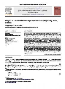
Fig. 3. Computational results for the total step and execution times for Problem 1.

Problem 1. Nonlinear non-stiff Krogh’s problem: y0i = −βi yi + y2i ,

yi (0) = −1, [0, 20],

β1 = β2 = 0.2,

β3 = 0.3,

i = 1, 2, 3, 4

β4 = 0.4.

Exact solution: yi (x) =

βi 1 + ci eβi x

,

ci = −(1 + βi ).

Source: Johnson and Barney [11]. Problem 2. A two-body orbit problem (mildly stiff): y01 = y3 ,

y02 = y4 ,

y1 (0) = 1,

y03 = −

y1

, 3

r y3 (x) = 0,

y2 (0) = 0,

y04 = −

y2

, 3

q

y21 + y22 r y4 (x) = 1, [0, 20]. r =

Exact solution: y1 (x) = cos(x),

y2 (x) = sin(x)

y3 (x) = − sin(x),

y4 (x) = cos(x).

Source: Hairer et al. [12]. Problem 3. Linear non-stiff complex eigenvalues: y01 = −Ay1 + By2 ,

y02 = −By1 − Ay2 ,

√

A = C = 1,

B=D=

y1 (0) = 1,

y2 (0) = 1,

y03 = −Cy3 + Dy4 ,

y04 = −Dy3 − Cy4

3 y3 (0) = 1,

y4 (0) = 1, [0, 20].

Exact solution: y1 (x) = e−Ax (cos Bx + sin Bx),

y2 (x) = e−Ax (cos Bx − sin Bx)

y3 (x) = e−Cx (cos Dx + sin Dx),

y4 (x) = −e−Cx (cos Dx − sin Dx).

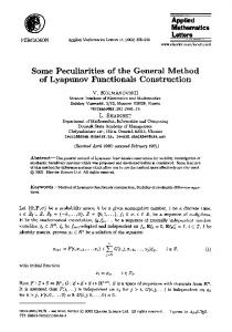
Source: Johnson and Barney [11]. The code was written in C language and all computations were carried out with a DYNIX/ptx operating system. The numerical results for the above test problems are tabulated in Tables 1–3. Table 4 gives the ratio of the total steps (Rstep) and execution times (Rtime) for the 4PG code compared to the 4P1FI code, for solving Problems 1–3. The results for the total steps and execution times for the given problems are also presented in the histograms and graph lines in Figs. 3–5. In Figs. 3–5, it is apparent that method 4PG required fewer total steps compared to method 4P1FI in most tolerances. It can be seen that the execution times of 4PG for solving the given problems are shorter than those for 4P1FI. Tables 1–3, show that for all test problems the total number of steps and function calls for the 4PG method are less than those for the 4P1FI method. The execution times for the 4PG method for solving all the given problems are shorter than those for 4P1FI in all tolerances. The maximum errors of 4PG are comparable to or better than those for the 4P1FI code. In Table 4, the ratios being greater than 1 show the advantage of 4PG over 4P1FI.


2393

Fig. 4. Computational results for total step and execution times for Problem 2.

Fig. 5. Computational results for total step and execution times for Problem 3.

Table 1 Numerical results from 4PG and 4P1FI methods for solving Problem 1. TOL 10

−2

10−4 10−6 10−8 10−10

MTD 4P1FI 4PG 4P1FI 4PG 4P1FI 4PG 4P1FI 4PG 4P1FI 4PG

TS 28 19 34 23 43 31 53 44 74 62

FS

MAXE

0 0 0 0 0 0 0 0 0 0

7.40 × 10 6.36 × 10−5 7.96 × 10−7 4.88 × 10−7 6.46 × 10−9 3.76 × 10−9 4.04 × 10−11 5.05 × 10−11 3.31 × 10−13 6.69 × 10−13 −5

FN

TIME

403 259 487 307 611 419 819 595 1115 847

1350 742 1078 641 1296 841 1677 1167 2135 1629

6. Conclusion and future work In this paper, a four-point four-step method is developed for solving systems of ODEs. From the numerical results we can conclude that the method has superiority in terms of total number of steps, maximum errors and execution times over the 4P1FI code given in [9]. However, we emphasize that there are some other variable step size methods in the literature devised by other authors. Cong and Xuan in [13] have mentioned that the explicit RK codes DOPRI5 and DOP853 are currently known as being the most efficient integrators for non-stiff first-order ODEs. These codes are embedded explicit RK methods due to Dormand and Prince, with step size control and dense output, and coded by Hairer and Wanner (see [12]). Our future work will

2394


Table 2 Numerical results from 4PG and 4P1FI methods for solving Problem 2. TOL

MTD

TS

FS

MAXE

FN

TIME

10−2

4P1FI 4PG 4P1FI 4PG 4P1FI 4PG 4P1FI 4PG 4P1FI 4PG

23 23 27 25 32 45 57 56 69 68

0 0 0 0 0 0 0 0 0 0

8.49 × 10−3 3.91 × 10−3 2.34 × 10−4 3.11 × 10−4 2.09 × 10−5 1.39 × 10−7 4.50 × 10−8 3.63 × 10−8 1.80 × 10−9 2.16 × 10−9

519 387 631 463 919 619 1231 919 1575 1319

1661 1174 1552 1096 1929 1533 2724 2119 3430 2874

10−4 10−6 10−8 10−10

Table 3 Numerical results from 4PG and 4P1FI methods for solving Problem 3. TOL

MTD

TS

FS

MAXE

FN

TIME

10−2

4P1FI 4PG 4P1FI 4PG 4P1FI 4PG 4P1FI 4PG 4P1FI 4PG

32 22 28 29 37 36 52 50 71 68

0 0 0 0 0 0 0 0 0 0

3.08 × 10−4 8.31 × 10−4 2.14 × 10−5 6.97 × 10−6 1.02 × 10−7 3.52 × 10−8 3.58 × 10−10 5.70 × 10−10 1.15 × 10−11 1.13 × 10−11

751 511 787 559 955 679 1219 899 1619 1247

2405 1735 1899 1709 2457 2097 3052 2775 4024 3809

10−4 10−6 10−8 10−10

Table 4 The ratios of total steps and execution times for the 4P1FI method to those for the 4PG method. TOL

−2

10 10−4 10−6 10−8 10−10

Problem 1

Problem 2

Problem 3

Rstep

Rtime

Rstep

Rtime

Rstep

Rtime

1.47 1.48 1.38 1.20 1.19

1.81 1.68 1.54 1.43 1.31

1.00 1.08 0.71 1.01 1.01

1.41 1.41 1.25 1.28 1.19

1.45 0.96 1.02 1.04 1.04

1.38 1.11 1.17 1.09 1.05

be devoted to investigating the performance of the method proposed in this paper compared against those of the above mentioned codes. Acknowledgements This research was supported by the Ministry of Higher Education under FRGS Grant 01-09-09-84FR. The authors wish to thank the referees for their careful reading of the manuscript and valuable comments. References [1] [2] [3] [4] [5] [6] [7] [8] [9] [10] [11] [12] [13]

K. Burrage, Efficient block predictor–corrector methods with a small number of corrections, J. Comput. Appl. Math. 45 (1993) 139–150. W.E. Milne, Numerical Solution of Differential Equations, Wiley, New York, 1953. J.B. Rosser, A Runge–Kutta for all seasons, SIAM Rev. 9 (1967) 417–452. L.F. Shampine, H.A. Watts, Block implicit one-step methods, Math. Comp. 23 (1969) 731–740. P.J. Houwen, P.B. Sommeijer, block Runge–Kutta methods on parallel computers, Report NM-R8906, Center for Mathematics and Computer Science, Amsterdam, 1989. Z. Omar, Developing Parallel Block Methods for Solving Higher Order ODEs Directly, Ph.D. Thesis, University Putra Malaysia, Malaysia, 1999. Z.A. Majid, Parallel block methods for solving ordinary differential equations, Ph.D. Thesis, University Putra Malaysia, 2004. Z.A. Majid, M. Suleiman, Performance of 4-point diagonally implicit block method for solving ordinary differential equations, Matematika 22 (2) (2006) 137–146. Z.A. Majid, M. Suleiman, Implementation of four-point fully implicit block method for solving ordinary differential equations, Appl. Math. Comput. 184 (2007) 514–522. Z.A. Majid, M. Suleiman, Z. Omar, 3-point Implicit Block Method for Solving Ordinary Differential Equations, Bull. Malays. Math. Sci. Soc. (2) 29 (1) (2006) 23–31. A.I. Johnson, J.R. Barney, Numerical solution of large systems of stiff ordinary differential equations, in: L. Lapidus, W.E. Schiesser (Eds.), Modular Simulation Framework, Numerical Methods for Differential Systems, Academic Press Inc., New York, 1976, pp. 97–124. E. Hairer, S.P. Norsett, G. Wanner, Solving ordinary differential equations I, in: Nonstiff Problems, 2nd ed., Springer-Verlag, Berlin, 1993. N.H. Cong, L.N. Xuan, Twostep-by-twostep PIRK-type PC methods with continuous output formulas, J. Comput. Appl. Math. 221 (2008) 165–173.