Journal of Computational and Applied Mathematics

Journal of Computational and Applied Mathematics 344 (2018) 356–366

Contents lists available at ScienceDirect

Journal of Computational and Applied Mathematics journal homepage: www.elsevier.com/locate/cam

Adaptive numerical approach based upon Chebyshev operational vector for nonlinear Volterra integral equations and its convergence analysis K. Maleknejad *, R. Dehbozorgi School of Mathematics, Iran University of Science and Technology, Narmak, Tehran 16844, Iran

article

a b s t r a c t

info

Article history: Received 16 April 2016 Received in revised form 31 December 2017 Keywords: Nonlinear Volterra integral equations Operational vector Chebyshev polynomials Convergence analysis

In the current paper, we present a direct numerical scheme to approximate a secondkind nonlinear Volterra integral equations (NVIEs). The scheme is based upon shifted Chebyshev polynomials and its operational matrices which eventually leads to the sparsity of the coefficients matrix of obtained system. The main idea of the proposed approach is based on a useful property of Chebyshev polynomials that yields to construct a new operational vector. This vector eliminates any requirement of using projection methods and also enhances the accuracy vs. other methods applied projection methods. The constructive technique and the convergence analysis of this approach under the L2w -norm are also described. Numerical experiments and comparisons confirm the applicability and the validity of the presented scheme. © 2018 Elsevier B.V. All rights reserved.

1. Introduction The Volterra integral equation is one of the important subjects of applied mathematics which occurs as a reformulation of ordinary or partial differential equation, or directly appears as a mathematical model of numerous applications in engineering, mathematical physics, economics, biology and etc. Recent researches in this regard include projection methods [1–4], wavelet methods [5,6], block pulse function [7], Bernstein’s approximation [8,9], triangular function method [10], radial basis functions (RBFs) [11]. Some of these methods are applicable only to linear integral equations. In the general case, these numerical schemes convert the integral equations to a system of linear or nonlinear algebraic equations. An orthogonal basis has the advantage that it guarantees the stability of the matrix equations [12]. A review of recently developed nonlinear analytical techniques can be found in [13]. In this article, a new computational method is presented for the following nonlinear Volterra integral equation of the second kind (NVIE2)

∫

t

k(x, t)G(u(x))dx,

u(t) = g(t) +

t ∈ D := [t0 , tf ]

(1)

t0

where g(t) ∈ H function u(t).

*

m1

(D), k(x, t) ∈ H

m2

(D2 ) are known functions and G(u(x)) is an algebraic nonlinear function of the unknown

Corresponding author. E-mail addresses: [email protected] (K. Maleknejad), [email protected] (R. Dehbozorgi). URL: http://webpages.iust.ac.ir/maleknejad (K. Maleknejad).

https://doi.org/10.1016/j.cam.2018.05.040 0377-0427/© 2018 Elsevier B.V. All rights reserved.

K. Maleknejad, R. Dehbozorgi / Journal of Computational and Applied Mathematics 344 (2018) 356–366

357

Chebyshev polynomials (CP) play a crucial role in approximation theory and in some quadrature rules for numerical integration. Since these polynomials are defined over the interval [−1, 1], then shifted Chebyshev polynomials (SCP) are used for interval D. In the present paper, we attempt to describe an efficient direct algorithm to approximate Eq. (1) based on these polynomials by introducing a new operational vector which is implied from one of the unique properties of Chebyshev polynomials. The operational vector overcomes the difficulties arising in the nonlinear part and also reduces the error of applying the projection methods such as collocation method [1–3], tau method [4]. In [14], the existence of these types of nonlinear equations has been discussed. This paper is organized as follows: Section 2 is devoted to state the basic concepts about the shifted Chebyshev polynomials and how to approximate the functions in terms of these polynomials. In addition, an efficient operational vector which is the key of our main idea is introduced. In Section 3, we verify how to derive the approximation solution by our proposed scheme. The convergence of the scheme is analyzed in Section 4. Finally, in Section 5 the numerical results are reported to demonstrate the accuracy and the applicability of the scheme in comparison with some recent methods [1–6,10]. 2. Properties of shifted Chebyshev polynomials Definition 2.1 ([15]). Chebyshev polynomials of the first kind (CP1) of degree m are defined over the interval [−1, 1] as

φm (x) = cos(mθ ),

θ = Arc cos(x),

or with its recursive formula can be interpreted as

φ0 (x) = 1, φ1 (x) = x, φm (x) = 2xφm−1 (x) − φm−2 (x). √

The orthogonality condition for φ (x) is satisfied with respect to the weight function w (x) = ( 1 − x2 )−1 as follows

⟨φi (x), φj (x)⟩w =

{

1

∫

w(x)φi (x)φj (x)dx = δi,j −1

π, π , 2

i = 0, i ̸ = 0.

Definition 2.2 ([16]). Shifted Chebyshev polynomials of degree m are defined over the interval D as follows Tm (t) = φm (

2

(t − t0 ) − 1) = φm (A(t − t0 ) − 1),

tf − t0

where A=

2 tf − t0

,

(2)

and so the weight function for SCP is described as

w ˜ (t) := w(A(t − t0 ) − 1) = √

tf − t0

2 (t − t0 )(tf − t)

.

One of the important properties of CP is completeness, therefore SCP also form a complete orthogonal set, that is, every f ∈ L2 (D) can be represented as an infinite series f (t) =

∞ ∑

cr Tr (t),

r =0

where the coefficient ci can be determined as ci =

⟨f (t), Ti (t)⟩w˜ . ⟨Ti (t), Ti (t)⟩w˜

(3)

Moreover, the orthogonality condition of SCP is as

⟨Ti (x), Tj (x)⟩w˜ =

∫

tf t0

w ˜ (x)Ti (x)Tj (x)dx =

δi,j A

{

π, π , 2

where A is defined in Eq. (2) and δ is Kronecker delta.

i = 0, i ̸= 0

(4)

358


2.1. The SCP operational matrix of integration Let T(t) = [T0 (t), T1 (t), . . . , TN −1 (t)]T be an N-vector of SCP. The SCP operational matrix of integration was derived in [16, p. 117] as follows

∫

t

T(s)ds ≃ P T(t),

(5)

t0

where

⎛

1

1

⎜ −1 ⎜ ⎜ ⎜ 4 ⎜ ⎜ −1 ⎜ ⎜ 3 1⎜ .. P= ⎜ A⎜ ⎜. ⎜ ⎜ (−1)N −1 ⎜ ⎜ (N − 1)(N − 3) ⎜ ⎜ ⎝ (−1)N

0 1

0

4

−1

0

2

N(N − 2)

0

···

0

0

0

0

···

0

0

···

0

0

.

.. .

⎟ ⎟ ⎟ ⎟ ⎟ ⎟ ⎟ 0 ⎟ ⎟ ⎟ .. ⎟ . ⎟ ⎟ ⎟ 1 ⎟ ⎟ 2(N − 1) ⎟ ⎟ ⎠

1 6

.. .

.. .

.. .

0

0

0

···

0

0

0

···

..

−1 2(N − 3) 0

⎞

0

0

−1 2(N − 2)

(6)

0

where A is a constant defined in (2). The operational matrix is implied by the differential recurrence relation Tr (t) =

1

(

T˙r +1

A 2(r + 1)

−

T˙r −1 2(r − 1)

).

Also regarding (6), one can conclude that

∫

t

TN −1 (s)ds = t0

1

(−1)

N

1 1 ( T (t) − T (t) + T (t)), A N(N − 2) 0 2(N − 2) N −2 2N N

N ≥ 3.

(7)

2.2. The SCP operational vector of product This section is devoted to introduce the product operational vector for SCP. To the best of our knowledge, only block pulse functions have this product operational vector as an explicit formula which is the consequences of the disjointness of these functions, for more details see [17]. This vector representation makes them popular and efficient basis functions for solving integral equations [18,19]. In [2,20], Maleknejad et al. apply this property for the Legendre polynomials and Chebyshev polynomials, but they have no closed formulas and have to evaluate it manually which is difficult and time-consuming. Here, we introduce this operational vector as an explicit and closed formula for SCP with respect to the following property Ti (t)Tj (t) =

1 2

(Ti+j (t) + T|i−j| (t)).

(8)

Let B = (bi,j )N ×N , then by using the above property, we can achieve the product operational vector for T(t) as follows T ˆ T (t)BT(t) = BT(t) ,

(9)

ˆ can be interpreted as where the entries of the vector B ˆ B(k) =

N ∑

ci,j bi,j ,

k = 1, . . . , N ,

(10)

i,j=1

where

⎧ 1, ⎪ ⎪ ⎨ 1 ci,j = , ⎪ ⎪ ⎩2 0,

A ∧ B, A ∨ B,

other w ise.

For brevity, two conditions |i − j| = k − 1 and i + j − 2 = k − 1 are considered as A and B, respectively. The logical symbol ∨ denotes that the expression A ∨ B is true if and only if just one of these conditions is true.


359

Using this vector, the positive integer power of a function can be approximated by an explicit formula as follows

[u(t)]p ≃ U∗p T(t).

(11)

Another advantage of this vector is to omit one of the basis vector T(t) in Eq. (9) which is explained in more detail in next sections. Remark 2.3. It should be noticed that due to the same property (8) for SCP and CP, their product operational vectors are equal.

2.3. The SCP operational matrix of product By applying the main characteristic of shifted Chebyshev polynomials (8), the SCP product operational matrix is as follows T

T

T(t)T (t)C = C T(t)

(12)

where C = [c0 , c1 , . . . , cN −1 ] is a vector and C is a square matrix of order N as 2c0 ⎜2c1

c1 2c0 + c2

⎛

⎜. ⎜. ⎜. 1⎜ C = ⎜2ci 2 ⎜. ⎜. ⎜. ⎝2c

.. .

ci−1 + ci+1

.. .

N −1

2cN −2

ci

··· ··· .. . ··· .. . ··· ···

cN −2 + cN cN −1

ci−1 + ci+1

.. .

2c0 + c2i

.. .

cN −i−1 cN −i

··· ··· ··· ··· .. . ··· ···

cN −2

cN −2 + cN

.. .

cN −i−1

.. .

2c0 c1

cN −1 cN −1 ⎟

⎞

..⎟ ⎟ .⎟ ⎟ cN −i ⎟ , ..⎟ ⎟ .⎟ ⎠ c

(13)

1

2c0

where i = [ N2 ]. As we expected by noting Remark 2.3, the SCP product operational matrix C is equal to the CP product operational matrix which can be found in [2]. 3. Outline of the numerical scheme In this section, we are going to introduce an appropriate numerical solution of the NVIE2 (1). All the functions u(t), g(t), k(s, t) and (u(t))r can be expanded with respect to shifted Chebyshev polynomials T(t) as T

u(t) ≃ uN (t) = U T(t), T

k(s, t) ≃ kN (s, t) = T (s)KT(t),

(14)

T

g(t) ≃ gN (t) = G T(t), ∗

(u(t))r ≃ urN (t) = Ur T(t). The large variety of nonlinearities could occur in practice, but we consider the algebraic ones as follows G(u(s)) =

n ∑

αr ur (s).

(15)

r =0

Hence, Eq. (1) is of the following form u(t) = g(t) +

n ∑

αr

r =0

t

∫

k(s, t)ur (s)ds,

t ∈ D.

(16)

t0

Now, in order to derive the unknown function u(t) in Eq. (16), we approximate all functions using Eq. (14) as follows T

T

U T(t) = G T(t) +

n ∑

T

αr (T (t)

∫

t

K T(s) U∗r T(s)ds), t0

r =0

or, regarding to the product operational matrix (12), T

T

U T(t) = G T(t) +

n ∑ r =0

T

αr (T (t)

∫

t

K Ur T(s)ds). t0

(17)

360


Using the operational matrix of integration (5), the above equation can be written as T

n ∑

T

U T(t) = G T(t) +

T

αr (T (t) K Ur P T(t)).

(18)

r =0

Now, let Br := KUr P, then our introduced operational vector (9) simplifies the above expression as the following matrix representation T

T

U =G +

n ∑

αr Bˆ r ,

(19)

r =0

ˆ r is a nonlinear vector in terms of entries of the U. Owing to the structure of the system (19), we employ the where B Newton’s iteration method for seeking the unknown vector U, then the desired approximation uN (t) can be obtained from T uN (t) = U T(t). ˆ r in (19), we have to use the collocation Remark 3.1. It should be noted that if we do not apply the operational vector B method analogy the scheme in [2]. In other words, an improvement of scheme [2] using operational vector is investigated. 4. Convergence analysis 2

In this section, we analyze the convergence of the presented scheme with respect to L -norm. To this end, we prepare an w ˜

2

error bound for using the operational matrix of integration in the approximation procedure under the L -norm. Throughout w ˜

2

this paper, the norm ∥.∥ denotes the L -norm which is defined as follows w ˜

∥.∥ =

∫ (

) 12

2

(.) w ˜ dx

.

(20)

D

Definition 4.1 ([21]). A function g : D → R belongs to Sobolev space W p derivatives) of g, g (i) , lie into L (D) for all 0 ≤ i ≤ m with the norm

∥g ∥W m,p =

m ∑

m,p

(D), if all distributional derivatives (weak

∥g (i) ∥Lp ,

i=0 2

where ∥.∥L denotes the Lebesgue norm. Furthermore, since L (D) is a Hilbert space, then W p

m,2

m

(D) := H (D).

p

Theorem 4.2 ([21]). If f has p continuous derivatives, f ∈ C (D), then the error estimate between Chebyshev expansion of f and f is as follows c LnN

T

∥f (t) − C T(t)∥∞ ≤

Np

.

(21)

m

n

2

Lemma 4.3 ([21]). If f ∈ H (Ω ), Ω ⊆ R and fN be the best approximation polynomial of f in L -norm, then w ˜

w ˜

∥f − fN ∥ = O(N −m ). m

Theorem 4.4. Suppose that f (t) ∈ H (D) and fN (t) = w ˜

t

∫ E=∥

t

∫

r =0

T

cr Tr (t) = F T(t) be the best approximation of f . The error estimate

T

F T(t) ds∥ ≤ CN −m

f (s)ds − t0

∑N − 1

(22)

t0

holds, where C is a constant that depends on A. T

Proof. Let FN (s) = |f (s) − F T(s)|, then by definition (20), we have t

∫ E =∥

=

∫ (

∫

t

t0 tf t0

∫

T

t0

∫ (

t

F T(s) ds∥ = ∥

f (s)ds − t

FN (s) dt

FN (s) ds∥ t0

)2

w ˜ (t) dt

) 21

(23)

.

t0

Now by applying Jenson’s inequality [22, p. 47], we know that

∫

t

FN (s)ds)2 ≤ (t − t0 )

( t0

∫

t

t0

2

FN (s)ds ≤

2 A

∫

t t0

2

FN (s)ds.

(24)


361

Now using Eqs. (23) and (24), we get tf

∫

2

t

∫

2

2

FN (s)ds) w ˜ (t)dt ≤

(

E =

A

t0

t0

2

≤ =

A

t

t

( t0

t

∫ 0 tf

2

FN (s)ds)w ˜ (t)dt

∫

2

FN (s)ds)(

( t

∫0

A2

2

FN (s)ds)w ˜ (t)dt

∫ 0tf ∫ 0tf

2π

=

t

∫ (

A 2

tf

∫

tf

t0

tf

(25)

w ˜ (t)dt)

t0

2

FN (s)ds.

where the last equality follows from the orthogonality condition (4), i.e., tf

∫

w ˜ (t)dt =

∫

t0

tf

T0 (t)T0 (t)w ˜ (t)dt =

t0

π A

.

Since w ˜ (s) > 1 over the interval D, then 2

E
N0 ,

∥FN (s)∥ = CN −m = O(N −m ) where C is a constant. Consequently,

√ E≤

C

2π 2

A

N −m = O(N −m ).

(26)

The following theorem is to derive an error bound for the SCP operational matrix of integration. m

Theorem 4.5. Assume that function f ∈ H (D) and TN (t) = [T0 (t), T1 (t), . . . , TN −1 (t)] is a vector of shifted Chebyshev w ˜

T

∑N −1

2

polynomials. If fN (t) = -norm, then the error of using the operational r =0 cr Tr (t) = F TN (t) be the best approximation of f in Lw ˜ matrix of integration P defined in (6) satisfies in the following inequality:

∫

t

T

f (s)ds − F PTN (t)∥ ≤ Ef ,

∥

(27)

t0

where Ef = CN −k +

| cN − 1 | 2AN

and |cN −1 | is a finite constant that depends on f (t) and N.

Proof. The expression (5) in the exact form can be written as:

∫

t

TN (t) = PN ×(N +1) TN +1 (t) t0

where we just denote the indexes to verify the dimension of the T(t) and matrix P. Hence, by regarding Eq. (7), one can conclude the error estimation of the relation (5) is as follows:

∫

t

TN (t)dt − PN ×N TN (t) = t0

TN (t) 2AN

.

Therefore,

∫

t

T

T

∫

T

t

F T(s)ds − F PT(t)∥ = ∥F (

∥ t0

T(s)ds − PT(t))∥ t0

∫

tf

T (t)

2

1

w ˜ (t)|cN −1 ( N )| dt) 2 2AN t0 √ |cN −1 | π = . = (

2AN

2A

(28)

362


Note that the orthogonality condition (4) is used for the last inequality. Finally, with triangular inequality, Theorem 4.4 and Eq. (28), one can derive t

∫

t

∫

T

f (s)ds − F PT(t)∥ ≤ ∥

∥

∫ 0t

T

F T(s)ds∥

f (s)ds − t0

t

t0

t

∫

T

T

F T(s)ds − F PT(t)∥

+ ∥

(29)

t0

√ |c | π ≤ C1 N −m + N −1 . 2AN

2A

≤ C1 N −m + C2 |cN −1 |N −1 where C1 and C2 are constants that depend on A. Remark 4.6. It is worthwhile noting that Eq. (29) has the order O(min{N −m , O(cN −1 )N −1 }) where O(cN −1 ) depends on p f (t) ∈ H m (D). In an especial case, if f ∈ C p (D), then f ∈ H (D) and so p ≤ m. Therefore, regarding to Theorem 4.2 and ln(N) < N, we have O(cN −1 ) = O(N −p+1 ). Consequently, Eq. (29) is the order of O(N −p ). In order to investigate the convergence analysis, we need the error bound of using operational matrix like Theorem 4.5 for bivariate functions which is stated in the following corollary. m

Corollary 4.7. Assume that a bivariate function L(x, t) ∈ H (D2 ) and TN (t) = [T0 (t), T1 (t), . . . , TN −1 (t)] be a vector of SCP. If T

2

w ˜

TN (x)LTN (t) be the best approximation of L(x, t) in L -norm, then the error of using the operational matrix of integration P defined w ˜ in (6) satisfies in the following inequality:

∫

t

∥ t0

T

L(s, t)ds − TN (t)LPTN (t)∥ ≤ EL ,

where EL = CN

−m 2

+

|lNN | 2AN

.

√π 2A

(30)

, L = (li,j )N ×N and |lNN | is a finite constant that depends on L(x, t) and N.

Proof. According to Theorem 4.4 and 4.5, the result is obtained. Theorem 4.8. Assume that the integral equations (1) with algebraic nonlinearity are uniquely solvable and u(x) be the exact m m solution. Also, we assume that the functions g(t) ∈ Hw˜ 1 (D) and k(x, t) ∈ Hw˜ 2 (D2 ), then the present scheme is convergent, i.e.,

∥u(t) − uN (t)∥ ≤ CN −m1 +

n ∑

αr Ekur

(31)

r =0

where Ekur is defined in Corollary 4.7 and C is an appropriate constant. Proof. In Eq. (16), let Lr (x, t) := k(x, t)ur (x), i.e., u(t) = g(t) +

n ∑

αr

r =0

∫

t

Lr (x, t)dx.

(32)

t0 T

Then, by the present scheme u(t) can be approximated directly with uN (t) = U TN (t) using operational matrix of integration as uN (t) = gN (t) +

n ∑

αr T(t)Lr PT(t)

(33)

r =0

where like Eq. (14), Lr (x, t) ≃ (Lr )N (x, t) = kN (x, t)urN (x) = TN (x)Lr TN (t). In order to obtain the error of the present scheme, first we subtract Eq. (32) from Eq. (33), u(t) − uN (t) = g(t) − gN (t) +

n ∑ r =0

αr (

t

∫

Lr (x, t)dx − T(t)Lr PT(t)).

(34)

0

Since gN (t) = GT T(t) is the best approximation of g(t), so regarding to Lemma 4.3 we have

∥ g(t) − gN (t) ∥≤ cN −m1 .

(35)


363

Table 1 A comparison between the COV, collocation method [2] and Tau method [4] under L∞ -norm of Example 1. N

COV

Collocation method [2]

Tau method [4]

4 8 10 12 16

2.74e−04 2.28e−08 2.12e−10 1.71e−10 1.30e−10

2.04e−02 2.45e−05 1.02e−06 4.59e−07 2.48e−07

4.46e−03 6.66e−07 – 2.07e−11 6.50e−16

Using the triangular inequality and Eq. (35), we get

∥u(t) − uN (t)∥ ≤ ∥g(t) − gN (t)∥ +

n ∑

αr ∥

≤ cN

+

n ∑

αr ∥

Lr (x, t)dx − T(t)Lr PT(t)∥ 0

r =0

−m1

t

∫

(36)

t

∫

Lr (x, t)dx − T(t)Lr PT(t)∥. 0

r =0 m

m

Since the functions g(t) ∈ Hw˜ 1 (D) and k(x, t) ∈ Hw˜ 2 (D2 ), so u(x) ∈ H m (D) where m = min{m1 , m2 }. Also, we know that if p q p < q, then H ⊃ H . Hence, Lr (x, t) = k(x, t)ur (x) ∈ H s (D2 ) where s = min{m, m2 }. Now regarding to Corollary 4.7 for s 2 Lr (x, t) ∈ H (D ) we have

∥u(t) − uN (t)∥ ≤ cN −m1 +

n ∑

αr ELr

(37)

r =0

|(l

)r |

π NN . 2A , Lr = (lij )r ,1≤i,j≤N is an N × N matrix and |(lNN )r | is a finite constant that depends on where ELr = Ekur = CN −s + 2AN Lr (x, t) and N for all r = 0, 1, . . . , n. It should be noticed that all discussions in Remark 2.3 are also valid about the rate of convergence of the scheme in Eq. (37).

√

5. Numerical experiments In this section, numerical results will be presented in order to compare the performance of the new approach with other projection methods, specially collocation method [2]. To study the convergence behavior of our method, we use maximum absolute error (L∞ -norm) and/or L2w˜ -norm. In addition, for a sake of good comparison, we test and analyze the scheme in [2] for all examples. Let us call our approach as COV (Chebyshev Operational Vector) method. All calculations are supported with Mathematica 9. Example 1. Consider the following NVIE2 u(t) = 1 + sin2 (t) −

t

∫

3 sin(t − s)u2 (s)ds,

t ∈ [0, 1],

(38)

0

with exact solution u(t) = cos(t). The above example has been solved with miscellaneous methods [1,3,4,6]. In [1,3], multistep collocation methods are applied with M = 32 points and the absolute error of their approximate solutions has the orders O(10−6 ) and O(10−8 ), respectively. Also, Cubic B-spline iterative method with 10 iteration and M = 250 collocation points is of the order O(10−9 ). Table 1 demonstrates the comparison between the Chebyshev collocation method [2], Tau method using Chebyshev polynomials [4] and the present scheme. It can be easily seen that COV scheme is more accurate than the mentioned scheme for small N ≤ 10 which has low computational cost, but when we increase the N, then a little change happens. Hence, the best computational result of our scheme obtains with N = 10. Maybe, it is optimal N for our proposed scheme for this example. Although in this example, Tau scheme [4] has good accuracy when N increases, but the present scheme is more accurate than the other existing methods [1–4,6] with less used basis functions, low computational cost and small size of operational matrix, N ≤ 10. Example 2. Consider the following NVIE2 u(t) = 2t −

t4 2

+

1 4

t

∫

u3 (s)ds,

t ∈ [0, 1],

(39)

0

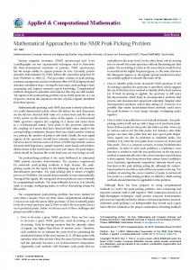
with exact solution u(t) = 2t. The approach presents the absolute error of order O(10−16 ) with a few terms (N = 4). Fig. 1 and Table 2 verify this claim.

364


Fig. 1. Absolute error between exact and approximate solutions (N = 4).

Table 2 A comparison between the COV and collocation method [2] under L∞ -norm and L2w -norm of Example 2. N =4

COV

[2]

L2w L∞

2.88e−16 2.95e−16

3.01e−02 4.57e−02

Table 3 A comparison between the COV and the collocation method [2] under L∞ norm of Example 3. N

COV

[2]

4 8

2.39e−05 1.99e−10

6.60e−03 2.45e−06

Example 3. Consider the following NVIE2 u(t) =

3 2

1

− e−2t − 2

t

∫

(u2 (s) + u(s))ds,

t ∈ [0, 1],

(40)

0

with exact solution u(t) = e−t . This example has been studied in [5,10] by using Haar wavelet method and the triangular function method, respectively. Their obtained absolute error has the order O(10−4 ) and O(10−3 ) with N = 32. Table 3 verifies that COV method is more accurate than those existing methods with less basis functions. Example 4 ([2]). Consider the following NVIE2 u(t) = 3t − 1 −

1 3

et (13 − e1+t + 12t + 9t 2 ) −

1 3

∫

t

e2t −x u2 (s)ds,

t ∈ [−1, 1],

(41)

−1

with exact solution u(t) = 3t − 1. Table 4 demonstrates the absolute error of the present approach and the collocation method [2] for different points in the interval [−1, 1]. It can be observed that our direct scheme is more accurate than [2]. Example 5. As a test example, consider the following NVIE2 t

∫

u2 (s)ds,

u(t) = f (t) + 4

(42)

0 2

2

2

where f (t) is determined such that the exact solution u(t) = te−t . Hence, f (t) = te−t + 41 (4te−2t −

√

√

2π erf ( 2t)).

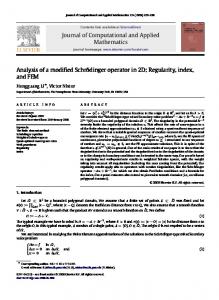
A comparison between our scheme and collocation method [2] is listed in Table 5 with respect to L2w -norm. Fig. 2 depicts the absolute error between exact and approximate solutions for various values of t and N = 10 where the error is of the order of O(10−8 ).


365

Table 4 A comparison of numerical L∞ -error of Example 4. t

COV

[2]

N =8

N = 10

N =8

N = 10

−1.0 −0.75 −0.5 −0.25 0.0 0.25 0.5 0.75 1.0

1.20e−05 4.51e−06 6.75e−07 7.67e−06 7.07e−07 9.92e−06 1.79e−05 1.49e−05 1.00e−05

9.82e−08 7.00e−08 6.35e−08 3.75e−08 5.14e−08 3.13e−08 6.51e−08 7.45e−08 4.53e−08

2.39e−06 6.63e−05 2.73e−04 3.61e−04 3.97e−04 1.28e−03 1.82e−03 2.18e−03 1.59e−03

2.42e−08 6.44e−09 3.04e−06 2.90e−06 1.18e−05 1.50e−05 2.94e−05 3.19e−05 2.49e−05

∥E ∞ ∥

2.30e−05

1.03e−07

3.02e−03

3.72 e−05

Table 5 A comparison of numerical L2w -error of Example 5. N

COV

[2]

4 6 8 10

9.34e−04 1.26e−05 1.74e−07 2.39e−08

3.44e−02 5.75e−03 7.96e−04 6.35e−05

Fig. 2. Absolute error between exact and approximate solutions (N = 10).

Remark 5.1. In all examples, the superiority of the Chebyshev operational vector method compared with the Chebyshev collocation method [2] is investigated. With less basis functions and low computational cost, the better results are obtained. 6. Conclusions A general formulation of operational vector based on shifted Chebyshev polynomials has been derived. A fast and accurate algorithm by using this vector for solving NVIEs is developed. Our approach has some advantages compared to the projection method used in [2] such as the simplicity of performing, ease of comprehending and high accuracy. A survey on the convergence of the present scheme is investigated. Numerical treatments confirm the validity and the applicability of the present method. Although, our discussion is restricted to Volterra integral equations of the second kind, but it can also be applied to other types of integral equations with some changes. References [1] D. Conte, B. Paternoster, Multistep collocation methods for volterra integral equations, Appl. Numer. Math. 59 (8) (2009) 1721–1736. [2] K. Maleknejad, S. Sohrabi, Y. Rostami, Numerical solution of nonlinear volterra integral equations of the second kind by using chebyshev polynomials, Appl. Math. Comput. 188 (1) (2007) 123–128. [3] C.-T. Sheng, Z.-Q. Wang, B.-Y. Guo, A multistep legendre–gauss spectral collocation method for nonlinear volterra integral equations, SIAM J. Numer. Anal. 52 (4) (2014) 1953–1980. [4] F. Ghoreishi, M. Hadizadeh, Numerical computation of the tau approximation for the volterra-hammerstein integral equations, Numer. Algorithms 52 (4) (2009) 541.

366


[5] I. Aziz, et al., New algorithms for the numerical solution of nonlinear fredholm and volterra integral equations using haar wavelets, J. Comput. Appl. Math. 239 (2013) 333–345. [6] K. Maleknejad, R. Mollapourasl, P. Mirzaei, Numerical solution of volterra functional integral equation by using cubic b-spline scaling functions, Numer. Methods Partial Differential Equations 30 (2) (2014) 699–722. [7] E. Babolian, A.S. Shamloo, Numerical solution of Volterra integral and integro-differential equations of convolution type by using operational matrices of piecewise constant orthogonal functions, J. Comput. Appl. Math. 214 (2) (2008) 495–508. [8] K. Maleknejad, E. Hashemizadeh, R. Ezzati, A new approach to the numerical solution of volterra integral equations by using bernsteins approximation, Commun. Nonlinear Sci. Numer. Simul. 16 (2) (2011) 647–655. [9] S. Bhattacharya, B. Mandal, Use of bernstein polynomials in numerical solutions of volterra integral equations. [10] K. Maleknejad, H. Almasieh, M. Roodaki, Triangular functions (tf) method for the solution of nonlinear volterra–fredholm integral equations, Commun. Nonlinear Sci. Numer. Simul. 15 (11) (2010) 3293–3298. [11] K. Parand, J. Rad, Numerical solution of nonlinear volterra–fredholm–hammerstein integral equations via collocation method based on radial basis functions, Appl. Math. Comput. 218 (9) (2012) 5292–5309. [12] L. Delves, J. Mohamed, Computational Methods for Integral Equations, Cambridge University Press, Cambridge, 1985. [13] J.-H. He, A review on some new recently developed nonlinear analytical techniques, Int. J. Nonlinear Sci. Numer. Simul. 1 (1) (2000) 51–70. [14] A. Karoui, On the existence of continuous solutions of nonlinear integral equations, Appl. Math. Lett. 18 (3) (2005) 299–305. [15] M. Abramowitz, I.A. Stegun, Handbook of Mathematical Functions with Formulas, Graphs, and Mathematical Table, Vol. 2172, Dover, New York, 1965. [16] K.B. Datta, B.M. Mohan, Orthogonal Functions in Systems and Control, Vol. 9, World Scientific, 1995. [17] Z. Jiang, W. Schoufelberger, M. Thoma, A. Wyner, Block Pulse Functions and their Applications in Control Systems, Springer-Verlag New York, Inc., 1992. [18] S. Hatamzadeh-Varmazyar, Z. Masouri, E. Babolian, Numerical method for solving arbitrary linear differential equations using a set of orthogonal basis functions and operational matrix, Appl. Math. Model. 40 (1) (2016) 233–253. [19] E. Babolian, Z. Masouri, Direct method to solve volterra integral equation of the first kind using operational matrix with block-pulse functions, J. Comput. Appl. Math. 220 (1–2) (2008) 51–57. [20] K. Maleknejad, B. Basirat, E. Hashemizadeh, Hybrid legendre polynomials and block-pulse functions approach for nonlinear volterra–fredholm integrodifferential equations, Comput. Math. Appl. 61 (9) (2011) 2821–2828. [21] A. Quarteroni, C. Canuto, M. Hussaini, T. Zang, Spectral Methods Fundamentals in Single Domains, Vol. 4, Springer Verlag, 2006, p. 16 8. [22] C. Niculescu, L.-E. Persson, Convex Functions and their Applications: A Contemporary Approach, Springer Science & Business Media, 2006.