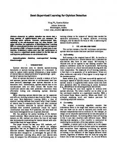
JP1.21
USING SUPERVISED LEARNING FOR SPECIFIC METEOROLOGICAL SATELLITE APPLICATIONS Richard L. Bankert and Jeffrey D. Hawkins Naval Research Laboratory, Monterey, CA
1. INTRODUCTION
2. GOES CLOUD CLASSIFICATION
Automated satellite interpretation algorithms that provide meteorological parameter estimation or diagnosis, in a timely manner, would be an invaluable asset to operational meteorologists, including those employed by the U.S. Navy. Two such algorithms currently being developed at the Naval Research Laboratory (NRL) are a cloud classifier and a tropical cyclone intensity estimation routine.
Taken from a time period of 1.5 years (Feb, 1999 through Aug, 2000), a training set of expertly-labeled 16x16 km samples (Figure 1) is created from GOES-8 and GOES-10 data for the daytime classifier. These training samples were independently classified by three different satellite interpretation experts. Only those samples given the same classification from all three experts were saved in the training set. The daytime training data was separated into two sets – land (5313 samples) and water (5937 samples). The nighttime classifier is currently in development.
These algorithms are developed using pattern recognition and supervised learning methodologies in which a set of training data is used to determine the characteristic patterns in the data that best discriminate the required output parameters. A nearest-neighbor routine is used to compute the similarities of the pattern or characteristic feature vector of a testing sample with those computed for the samples in the training set. The values or classes associated with one or more nearest neighbors within the training set are used as an estimate or classification of the testing sample. Expanding upon the cloud classification routine developed at NRL for Advanced Very High Resolution Radiometer (AVHRR) data (Tag et al. 2000), a 1nearest neighbor algorithm is developed for Geostationary Operational Environmental Satellite (GOES) data. For the daytime classifier, training sample feature vectors are computed using all five GOES spectral channels and can be applied to GOES8 (East) and GOES-10 (West) data. A testing (or operational) sample is classified with the same class as the nearest training sample in the multi-dimensional feature space. Given the fact that upper-level (nonprecipitating) clouds are essentially transparent within the passive microwave imagery (Hawkins et al. 1998), low-level structure and circulation of tropical cyclones are apparent in Special Sensor Microwave Imager (SSM/I) data. Taking advantage of these sensor characteristics, a K-nearest neighbor algorithm is developed to estimate the intensity of a tropical cyclone using 85-GHz and derived rain rate feature characteristics. As opposed to the single nearestneighbor used in the GOES cloud classifier, multiple neighbors are used to estimate the intensity of a testing (or operational) sample presented to the pattern recognition algorithm. Corresponding author address: Richard L. Bankert, Naval Research Laboratory, 7 Grace Hopper Ave., Monterey, CA 93943; e-mail:
[email protected]
Figure 1. GOES-10 image (central California coast) with red boxes indicating example 16x16 km boxes used as training samples in GOES cloud classifier. Using data from all five GOES channels, over 100 characteristic features are computed for each training sample. Some example features include maximum, minimum, mean, and standard deviation within the sample for each channel, visible channel textures (contrast, homogeneity, entropy, etc), latitude, and climatological sea surface temperature. Due to the fact that using all features degrades classifier performance (because of redundant and irrelevant information) and increases the time it takes to classify an image, a feature selection algorithm is applied to the training data to determine which subset of features optimizes classification accuracy. The
feature selection routine employs a variation of the backward sequential selection (BSS) algorithm and a 1nearest neighbor evaluation function. Using multiple feature subsets (as defined by the BSS algorithm), leave-one-out cross validation tests are performed using the training data set. The feature subset that produces the highest classification accuracy is the final selected set. For additional details on feature selection, see Aha and Bankert (1995) and Bankert and Aha (1996). Table 1 is a list of the selected features used in the GOES daytime classifier. With the selected feature subset, leave-one-out cross validation testing on both land and water training sets produced approximately 90% accuracy.
Feature Space
Cu
? Cu ? - Cu
Table 1. GOES Classifier Selected Features (Daytime) LAND Satellite (GOES-8, 10) Latitude Date (Season) Channel 2 minimum Channel 2 median Channel 3 median Channel 4 maximum Channel 4 range Channel 4 median Channel 5 minimum Channel 5 median 4 Channel 1 Textures
WATER Satellite (GOES-8, 10) Latitude Date (Season) Channel 1 median Channel 1 standard dev Channel 2 maximum Channel 2 mean Channel 3 maximum Channel 4 minimum Channel 4 range Channel 4 mean Ch4 – Ch5 mean 2 Channel 1 Textures Sea surface temp. (climo)
Class types include stratus (St), stratocumulus (Sc), cumulus (Cu), altocumulus (Ac), altostratus (As), cirrus (Ci), cirrocumulus (Cc), cirrostratus (Cs), cumulus congestus (CuC), cirrostratus associated with convection (CsAn), cumulonimbus (Cb), clear – bare ground or water body (Cl), ground snow (Sn), haze, sand, smoke, or dust (Hz), and sunglint (Sg). The chosen GOES cloud classifier is a 1-nearest neighbor algorithm due to the nonlinear, nonparametric nature of that algorithm. When an unclassified (testing or operational) 16x16 km GOES image sample is presented to the classifier, the similarity distance (1) is computed between that sample and each training set sample. Σ (testing featurei - training featurei )2
(1)
Each feature value used in (1) has been normalized, and the summation is over all features. See the 1nearest neighbor illustration in Figure 2.
Training sample (class known) Testing sample (class unknown) Figure 2. 1-nearest neighbor illustration. Testing sample is assigned to be Cu since the nearest training sample in feature space is a Cu type. 2.1 Real-Time Procedure For a complete GOES image classification, the 16x16 km classification boxes overlap each other such that each individual pixel is classified four times (two times for those pixel on image edges). The final classification of an individual pixel is determined by simple majority with ties broken by random selection. In addition, the training set choice (land or water) for classification boxes that fall over a coastline is determined by whichever type (land or water) covers the most pixels in that box. To present a more accurate representation of an image on the pixel level, the visible channel albedo (corrected for the solar zenith angle) is checked. If that value is less than 12%, then the pixel is re-classified as clear (Cl), regardless of the initial classification. Classification images are created using color-coded representations of the various classes. See Figures 3a and 3b for an example classification image. Known limitations of the GOES cloud classifier include the inability of the system, in its present form, to classify mixed cloud samples. Every 16x16 km box is classified with one of the “pure” classes even if it is a truly mixed sample. Situations such as thin cirrus over low clouds have been noted to be classified as As or Ac. The classifier is also limited by the amount and variability of the training data in each class. Representing the entire
Figure 3a. GOES visible image of Hurricane Flossie (28 Aug 2001,1700 UTC) in the Eastern Pacific Ocean. universal set of these classes as they are distributed over time (seasons) and space (latitude and longitude) is virtually impossible.
Figure 3b. Cloud Cassification image of Figure 3a.
A web page of real-time GOES daytime cloud classification output can be found at
http://www.nrlmry.navy.mil/sat-bin/clouds.cgi 2.2 Future Plans At the time of this writing, a GOES nighttime cloud classifier is being developed. Similar to the daytime classifier, expertly-labeled samples are being collected to provide land and water training sets with features to be computed from four of the five spectral channels (no visible channel data). Other plans include adding more geographic sectors to the GOES daytime cloud classification web page, examining the use of a surface albedo look-up table for pixel postprocessing (replacing 12% threshold), and developing automated classification algorithms for other geographical regions. Using data from the next generation of geostationary satellites would be the logical choice. These satellites include the European Meteosat Second Generation (MSG-1, August 2002 launch) and the Japanese Multifunctional Transport Satellite (MTSAT-1R).
Figure 4a. GOES-9 visible image of Typhoon Joan (2232 UTC 22 Oct 1997).
3. TROPICAL CYCLONE INTENSITY ESTIMATION Using SSM/I images to examine tropical cyclone structure has an advantage when compared with the limitations of other imagery types (Hawkins et al. 2001). Rainbands and a tropical cyclone center (when it exists) can be seen in the 85-GHz channel images when this structure is obscured by upper-level clouds as seen in visible and infrared imagery. Figure 4a-c illustrates this contrast in image types as the structure of Typhoon Joan is obscured in the visible and infrared imagery, but is apparent in the SSM/I 85-GHz image. Extracting this tropical cyclone structural information should be invaluable in developing an automated algorithm to estimate tropical cyclone intensity. Figure 4b. Infrared image of Typhoon Joan.
Table 2. SSM/I tropical cyclone selectedfeature list.
Figure 4c. SSM/I 85-GHz image of Typhoon Joan. The red areas indicate low brightness temperatures (high scattering due to large ice particles – convective precipitation) and blue areas indicate higher brightness temperatures (no or limited convection). The 85-GHz image data have a spatial resolution of 13 km x 15 km. Applying an interpolation algorithm (Poe, 1990), this data can be mapped to 1-2 km resolution. In addition to the 85-GHz data, rain rate “image” data is also used to extract feature characteristics that will be presented to a K-nearest neighbor algorithm. The rain rate “image” is a derived product from multiple SSM/I channels (Ferraro, 1997). SSM/I data from 175 tropical cyclones that comprise the period of 1988-2001 (and all relevant ocean basins) are used to train and test the tropical cyclone intensity estimation algorithm. Features are computed from 1297 SSM/I images that are 512x512 (km or pixels), centered on the tropical cyclone center, and have an associated best-track intensity. Over 100 characteristic features are computed from the 85-GHz and rain rate data. These features include spectral characteristics which are simple statistical measurements (maximum, minimum, mean, etc) of both 85 GHz and rain rate imagery. Textural feature values of the 85 GHz data are also computed. They provide a representation of the spatial distribution of the brightness temperatures within the image. Both the entire image and the inner 150x150 pixel region are divided into quadrants to extract information, in a general sense, about the convective organization in the tropical cyclone environment. Summations of all pixel values within each quadrant (both 85-GHz and rain rate) are saved as features. Features that are more tropical cyclone specific include enclosed eye (yes, no), size of enclosed eye, and banding and concentric ring features. Latitude,
Latitude Longitude |Yearday – 237| 85-GHz - Pixel summation – NE quadrant (512x512) 85-GHz - Pixel summation – NE quadrant (inner 150x150) 85-GHz - Segmented – normalized mean radius 85-GHz - Range of pixel values (512x512) 85-GHz - Range of temperature thresholds for which enclosed eye exists Rain rate - Average pixel value for those > 0 mm/hr (512x512) Rain rate - Number of pixels > 0 mm/hr (inner 150x150) Rain rate - Pixel summation – SE quadrant (512x512) Rain rate - Pixel summation – NW quadrant (inner 150x150) Rain rate - Mean pixel value (512x512) Rain rate - Mode pixel value (512x512) Rain rate - Banding feature – maximum summation of pixels on concentric rings (> 3 mm/hr)
longitude, and date (relative to peak activity) are also features. For additional details, see Bankert and Tag (2002). 3.1 Feature Selection and K-Nearest Neighbor In the same manner that it was applied to the GOES cloud classification training data, a feature selection algorithm is applied to the SSM/I tropical cyclone data. The notable difference here is that the evaluation function is a K-nearest neighbor algorithm. Using the single nearest-neighbor distance as the standard for inclusion, those training samples within a distance factor (1.75 X nearest-neighbor distance) are used to estimate the testing sample intensity. A simple averaging technique is performed on those K-nearest neighbor best track intensities. A leave-one-out cross validation test is applied to the training set (942 samples) and the RMSE is computed relative to each feature subset. The error for any given training sample is the difference between the K-NN estimated intensity and the best-track intensity. The reduced subset that produces the minimum RMSE after the search and Knearest neighbor evaluation is the final selected set. These selected features are listed in Table 2. 3.2 Results After the feature selection was completed, the training set increased by 237 samples (with the addition of tropical cyclones from 1999-2001) for a total of 1199 training samples. The testing set consists of 98 samples from four tropical cyclones: Hurricane Guillermo (August, 1997), Supertyphoon Oliwa
(September, 1997), Supertyphoon Paka (December, 1997), and Supertyphoon Babs (October, 1998). Using the 15 selected features as the representative vector for all of the training and testing samples, the testing set is presented to the K-nearest neighbor algorithm for evaluation. For the 98 testing samples, the overall RMSE is 19.0 kts with an average absolute error (AAE) of 15.3 kts, and an average percentage error (APE) of 25.0%. A majority of the samples (56%) had an intensity estimate within 15 kts of the best-track intensity, but 7% had an error greater than 30 kts. See Table 3 for a summary of the errors statistics for the four tropical cyclones in the testing set. Table 3. K-NN testing results (98 total samples). RMSE – Root Mean Square Error; AAE – Average Absolute Error; APE – Average Percent Error Tropical Cyclone Oliwa
RMSE (kts)
AAE (kts)
APE (kts)
(25 samples)
25.9
20.1
39.3
19.3
17.3
25.8
14.1
11.7
17.1
(22 samples)
14.3
12.2
17.5
OVERALL
19.0
15.3
25.0
Guillermo (24 samples)
Figure 5. A 512x512 85-GHz image of tropical cyclone Oliwa (2007 UTC 6 Sep 1997) at a time of relatively low intensity with extensive areas of cold brightness temperatures (blue and green areas) around the tropical cyclone center.
Paka (27 samples)
Babs
Most of the highest intensity estimation errors could be found with images associated with Oliwa. As an example, an 85-GHz image of Oliwa in the early stages of development (best-track – 35 kts) can be seen in Figure 5. The tropical cyclone intensity estimation algorithm is apparently doing a poor job of interpreting the convective area around the center of the cyclone. The algorithm produced an intensity estimate of 99.1 kts (64.1 kt error) for this image. Figure 6 is a time series plot of the best-track intensity and K-nearest neighbor intensity estimation for Paka. All four tropical cyclones had K-nearest neighbor time series plots that exhibited “spikes” along the timeline that are inconsistent with the best-track data. Although they contribute to the computed error, some of these spikes could be representing actual strengthening or weakening not captured in the smooth best-track data. 3.3 Discussion and Future Plans As noted in Bankert and Tag (2002), the snapshot approach (no historical information) used in this first version of the algorithm can be improved upon when adding past intensity to the set of features. This is one experiment that can be performed in future work on the recently expanded data set. Additionally, with the larger data set, a different feature subset may be needed.
While improvement in the methodology described here is needed, it is important to note that development and evaluation of the algorithm is dependent upon the accuracy of the best-track intensity of the training and testing samples. These intensities are estimated to have an error range of +/- 10-15 kts. Beyond experimentation with the current algorithm, investigating the use of other data sources and the use of output from other methodologies (e.g, Objective Dvorak Technique and AMSU) may be desired. Additionally, applying other pattern recognition and artificial intelligence technologies to create other algorithms (e.g, fuzzy rule-based system) should be done to compare performance and find the best approach. ACKNOWLEDGEMENTS The support of the sponsor, the Office of Naval Research, under Program Element 0602435N is gratefully acknowledged. The assistance of the satellite team (Code 7541) at NRL Monterey, Bob Fett, Ron Englebretson, and Robin Brody of Scientific Applications International Corp. (SAIC), and Marla Helveston of Anteon, Inc. is very much appreciated. REFERENCES Aha, D.W., and R.L. Bankert, 1995: A comparative evaluation of sequential feature selection algorithms. Learning from Data: Artificial Intelligence and Statistics V, D. Fisher and H.-J. Lenz, Eds., Springer-Verlag, 199-206.
Best Track
K-NN Estimate
140 130 120
Intensity (kts)
110 100 90 80 70 60 50 40 30 12/4
12/6
12/8
12/10
12/12
12/14
12/16
12/18
12/20
Image Time (1997)
Figure 6. Time series plot of best track intensity and K-nearest neighbor intensity estimate for Paka. Bankert, R.L., and D.W. Aha, 1996: Improvement to a neural network cloud classifier. J. Appl. Meteor., 35, 2036-2039. Bankert, R.L., and P.M. Tag, 2002: An automated method to estimate tropical cyclone intensity using SSM/I imagery. J. Appl. Meteor., 41, 461-472. Ferraro, R.R., 1997: Special sensor microwave imager derived global rainfall estimates for climatological applications. J. Geophys. Res., 102, 16715-16735. Hawkins, J.D., T.F. Lee, J. Turk, C. Sampson, J. Kent, and K. Richardson, 2001: Real-time internet distribution of satellite products for tropical cyclone reconnaissance. Bull. Amer. Met. Soc., 82, 567-578.
Hawkins, J.D., D.A. May, J. Sandidge, R. Holyer, and M.J. Heleveston, 1998: SSM/I-based tropical cyclone structural observations. Preprints, 9th Conference on Satellite Meteorology and Oceanography, Paris, France, Amer. Meteor. Soc., 230-233. Poe, G., 1990: Optimum interpolation of imaging microwave radiometer data. IEEE Tran. On Geosci. and Remote Sensing, GE-28, 800-810. Tag, P.M., R.L. Bankert, and L.R. Broday, 2000: An AVHRR multiple cloud-type classification package. J. Appl. Meteor., 39, 125-134.