award of any other degree or diploma at UNSW or any other educational ..... 3.5 A typical lifting structure; analysis is shown on the left side and synthesis ...... we note that Motion-JPEG2000 content does not involve any exploitation of inter- ...... Motion compensation is performed at 1/4 pixel precision with 7-tap interpolation.
School of Electrical Engineering and Telecommunications
JPEG2000-Based Scalable Interactive Video (JSIV) A thesis submitted for the degree of
Doctor of Philosophy
By
Aous Thabit Naman
Supervisor:
Prof. David Taubman
September 2010
PLEASE TYPE THE UNIVERSITY OF NEW SOUTH WALES Thesis/Dissertation Sheet
Naman First name: Aous Thabit Surname or Family name:
Other name/s:
Abbreviation for degree as given in the University calendar: School: of
Doctor of Philosophy (PhD)
Electrical Engineering and Telecommunications
Title: JPEG2000-Based
Faculty:
of Engineering
Scalable Interactive Video (JSIV)
Abstract 350 words maximum: (PLEASE TYPE)
Video is considered one of the main applications of today's Internet. Despite its importance, the interactivity available from current implementations is limited to pause and random access to a set of predetermined access points. In this work, we propose a novel and innovative approach that provides considerably better interactivity and we coin the term JPEG2000-Based Scalable Interactive Video (JSIV) for it. JSIV relies on three main concepts: Storing the video sequence as independent JPEG2000 frames to provide for quality and spatial resolution scalability as well as temporal and spatial accessibility. Prediction and conditional replenishment of precincts to exploit inter-frame redundancy. Loosely-coupled server and client policies. The philosophy behind the loosely-coupled client and server policies is that neither the server nor the client drives the video streaming interaction. Instead, we employ an intelligent server that optimally selects the number of quality layers for each precinct it transmits and decides on any side-information that needs to be transmitted, with an intelligent client that attempts to make most of the received (distorted) frames. For these policies to work, only intra-coded precincts are employed in JSIV. We solve the general JSIV optimization problem by employing Lagrange-style rate-distortion optimization in a two pass iterative approach. We show that this approach converges under workable conditions, and we also show that the optimal solution for a given rate is not necessarily embedded in the optimal solution for a higher rate. The flexibility of the JSIV paradigm enables us to use it in a variety of frame prediction arrangements. In this work, we focus only on JSIV with sequential prediction arrangement (similar to IPPP...) and hierarchical B-frames prediction arrangement. We show that JSIV can provide the sought-after quality and spatial scalability in addition to temporal and spatial accessibility. Consequently, we expect that real-time and interactive applications, such as teleconferencing and surveillance, would benefit most from JSIV. Experimental results show that JSIV's performance is slightly inferior to that of existing predictive coding standards in conventional streaming applications; however, JSIV performs significantly better when its scalability and accessibility features, such as region of interest, are employed. Declaration relating to disposition of project thesis/dissertation I hereby grant to the University of New South Wales or its agents the right to archive and to make available my thesis or dissertation in whole or in part in the University libraries in all forms of media, now or here after known, subject to the provisions of the Copyright Act 1968. I retain all property rights, such as patent rights. I also retain the right to use in future works (such as articles or books) all or part of this thesis or dissertation. I also authorise University Microfilms to use the 350 word abstract of my thesis in Dissertation Abstracts International (this is applicable to doctoral theses only).
…………………………………………………………… Signature
……………………………………..……………… Witness
……….……………………...…….… Date
The University recognises that there may be exceptional circumstances requiring restrictions on copying or conditions on use. Requests for restriction for a period of up to 2 years must be made in writing. Requests for a longer period of restriction may be considered in exceptional circumstances and require the approval of the Dean of Graduate Research. FOR OFFICE USE ONLY
Date of completion of requirements for Award:
THIS SHEET IS TO BE GLUED TO THE INSIDE FRONT COVER OF THE THESIS
COPYRIGHT STATEMENT ‘I hereby grant the University of New South Wales or its agents the right to archive and to make available my thesis or dissertation in whole or part in the University libraries in all forms of media, now or here after known, subject to the provisions of the Copyright Act 1968. I retain all proprietary rights, such as patent rights. I also retain the right to use in future works (such as articles or books) all or part of this thesis or dissertation. I also authorise University Microfilms to use the 350 word abstract of my thesis in Dissertation Abstract International (this is applicable to doctoral theses only). I have either used no substantial portions of copyright material in my thesis or I have obtained permission to use copyright material; where permission has not been granted I have applied/will apply for a partial restriction of the digital copy of my thesis or dissertation.'
Signed ……………………………………………...........................
Date
……………………………………………...........................
AUTHENTICITY STATEMENT ‘I certify that the Library deposit digital copy is a direct equivalent of the final officially approved version of my thesis. No emendation of content has occurred and if there are any minor variations in formatting, they are the result of the conversion to digital format.’
Signed ……………………………………………...........................
Date
……………………………………………...........................
ORIGINALITY STATEMENT ‘I hereby declare that this submission is my own work and to the best of my knowledge it contains no materials previously published or written by another person, or substantial proportions of material which have been accepted for the award of any other degree or diploma at UNSW or any other educational institution, except where due acknowledgement is made in the thesis. Any contribution made to the research by others, with whom I have worked at UNSW or elsewhere, is explicitly acknowledged in the thesis. I also declare that the intellectual content of this thesis is the product of my own work, except to the extent that assistance from others in the project's design and conception or in style, presentation and linguistic expression is acknowledged.’
Signed ……………………………………………..............
Date
……………………………………………..............
Abstract Video is considered one of the main applications of modern day’s Internet. Despite its importance, the interactivity available from current implementations is limited to pause and random access to a set of predetermined access points. In this work, we propose a novel and innovative approach which provides considerably better interactivity and we coin the term JPEG2000-Based Scalable Interactive Video (JSIV) for it. JSIV relies on three main concepts: storing the video sequence as independent JPEG2000 frames to provide for quality and spatial resolution scalability, as well as temporal and spatial accessibility; prediction and conditional replenishment of precincts to exploit inter-frame redundancy; and loosely-coupled server and client policies. The concept of loosely-coupled client and server policies is central to JSIV. With these policies, the server optimally selects the number of quality layers for each precinct it transmits and decides on any side-information that needs to be transmitted while the client attempts to make most of the received (distorted) frames. In particular, the client decides which precincts are predicted and which are decoded from received data (or possibly filled with zeros in the absence of received data). Thus, in JSIV, a predicted frame typically has some of its precincts predicted from nearby frames while others are decoded from received intra-coded precincts; JSIV never uses frame differences or prediction residues. The philosophy behind these policies is that neither the server nor the client drives the video streaming interaction, but rather the server dynamically selects and sends the pieces that, it thinks, best serve the client needs and, in turn, the client makes most
iii
of the pieces of information it has. The JSIV paradigm postulates that if both the client and the server policies are intelligent enough and make reasonable decisions, then the decisions made by the server are likely to have the expected impact on the client’s decisions. We solve the general JSIV optimization problem by employing Lagrange-style ratedistortion optimization in a two pass iterative approach. We show that this approach converges under workable conditions, and we also show that the optimal solution for a given rate is not necessarily embedded in the optimal solution for a higher rate. The flexibility of the JSIV paradigm enables us to use it in a variety of frame prediction arrangements. In this work, we focus only on JSIV with sequential prediction arrangement (similar to IPPP. . . ) and hierarchical B-frames prediction arrangement. We show that JSIV can provide the sought-after quality and spatial scalability in addition to temporal and spatial accessibility. We also demonstrate a novel way in which a JSIV client can use its cache in improving the quality of reconstructed video. In general, JSIV can serve a wide range of usage scenarios, but we expect that real-time and interactive applications, such as teleconferencing and surveillance, would benefit most from it. Experimental results show that JSIV’s performance is slightly inferior to that of existing predictive coding standards in conventional streaming applications; however, JSIV produces significant improvements when its scalability and accessibility features, such as the region of interest, are employed.
iv
To my wife Rasha, my parents Thabit and Ibtisam
v
Acknowledgments Many people contributed, directly and indirectly, to me finishing my doctoral degree. I am mostly indebted to my supervisor, Prof. David Taubman, for his continuous support and encouragement, for his guidance and wisdom throughout this work, and for his vision and enthusiasm regarding the work. His wide knowledge made the experience a more pleasant one. I am also thankful to him for providing me with financial assistance after my original scholarship ended. Moreover, I am thankful to him for providing me with the source code of the Kakadu software that was used in coding and decoding the JPEG2000 format throughout this work. I am thankful to the University of New South Wales (UNSW) for supporting me financially with the University Postgraduate Award (UPA) which made my study and research process possible. I would also like to express my appreciation of Tom Millet and Phil Allen for their kindness and genuine readiness to help, and although I had limited interaction with my co-supervisor, Dr. Vijay Sivaraman, due to the way the research evolved, I am thankful for his support and I wish to have a chance to work more closely with him in the future. I would also like to express my gratefulness to my wife for her support, understanding, and patience during the long hours I spent on this work, and also express my appreciation of the support my friends at UNSW gave and still giving, especially Reji Mathew and Jonathan Gan. I am also thankful to Dr. Reji Mathew for providing the source code for his embedded scalable motion encoder [57, 58] used for helping with the generation of motion vectors for this work.
vi
More importantly, I am grateful and thankful to my parents for their long and unfettered support during study and; in particular, my mother’s continuous encouragement throughout my doctoral degree. Lastly, I am grateful to God almighty that made all this possible.
vii
Contents 1 Introduction
1
1.1
Motivation
. . . . . . . . . . . . . . . . . . . . . . . . . . . . . . . . . .
1
1.2
Problem Statement . . . . . . . . . . . . . . . . . . . . . . . . . . . . . .
3
1.3
Our Contribution . . . . . . . . . . . . . . . . . . . . . . . . . . . . . . .
4
1.3.1
Publications . . . . . . . . . . . . . . . . . . . . . . . . . . . . . .
5
Outline of The Thesis . . . . . . . . . . . . . . . . . . . . . . . . . . . .
6
1.4
2 Introduction to JPEG2000-Based Scalable Interactive Video 2.1
Applications Where JSIV is Advantageous . . . . . . . . . . . . . . . . .
3 Scalable Interactive Image and Video Browsing 3.1
3.2
9 14 15
A Basic Compression System . . . . . . . . . . . . . . . . . . . . . . . .
15
3.1.1
Transformation . . . . . . . . . . . . . . . . . . . . . . . . . . . .
16
3.1.2
Quantization . . . . . . . . . . . . . . . . . . . . . . . . . . . . .
17
3.1.3
Source Coding . . . . . . . . . . . . . . . . . . . . . . . . . . . .
17
JPEG2000 Image Coding Standard . . . . . . . . . . . . . . . . . . . . .
18
3.2.1
Colour Transform
. . . . . . . . . . . . . . . . . . . . . . . . . .
19
3.2.2
Discrete Wavelet Transform . . . . . . . . . . . . . . . . . . . . .
20
3.2.3
Quantization . . . . . . . . . . . . . . . . . . . . . . . . . . . . .
26
3.2.4
Embedded Coding . . . . . . . . . . . . . . . . . . . . . . . . . .
27
3.2.5
Scalability and Accessibility Options in JPEG2000 . . . . . . . .
31
viii
3.3
3.4
Closed-Loop Predictive Video Coding (CLPVC)
. . . . . . . . . . . . .
32
3.3.1
Prediction Models and Arrangements . . . . . . . . . . . . . . .
35
3.3.2
CLPVC Shortcomings . . . . . . . . . . . . . . . . . . . . . . . .
37
Open-Loop Video Coding . . . . . . . . . . . . . . . . . . . . . . . . . .
38
3.4.1
Wavelet-Based Video Coding (WVC) . . . . . . . . . . . . . . . .
39
3.4.2
Scalable Video Coding (SVC) Extension of The H.264/AVC Standard . . . . . . . . . . . . . . . . . . . . . . . . . . . . . . .
42
3.5
Scalable Motion Coding (SMC) . . . . . . . . . . . . . . . . . . . . . . .
46
3.6
Distributed Video Coding (DVC) . . . . . . . . . . . . . . . . . . . . . .
48
3.7
Protocols for Interactive Image and Video Delivery . . . . . . . . . . . .
51
3.8
Other Recent Research in Interactive Video Browsing . . . . . . . . . .
52
4 JSIV without Motion Compensation
53
4.1
Oracle Client Policy . . . . . . . . . . . . . . . . . . . . . . . . . . . . .
54
4.2
Oracle Server Policy . . . . . . . . . . . . . . . . . . . . . . . . . . . . .
56
4.2.1
Rate-Distortion Optimization . . . . . . . . . . . . . . . . . . . .
56
4.2.2
Rate-Distortion Optimization in JSIV . . . . . . . . . . . . . . .
57
4.3
Actual Client and Server Policies . . . . . . . . . . . . . . . . . . . . . .
64
4.4
Distortion Estimation and Implementation Cost . . . . . . . . . . . . . .
70
4.5
Experimental Results and Usage Scenarios . . . . . . . . . . . . . . . . .
73
4.5.1
Individual Frame Retrieval . . . . . . . . . . . . . . . . . . . . .
78
4.5.2
Spatial and Temporal Scalability . . . . . . . . . . . . . . . . . .
79
4.5.3
Window of Interest . . . . . . . . . . . . . . . . . . . . . . . . . .
81
4.5.4
Use of Available Data . . . . . . . . . . . . . . . . . . . . . . . .
82
4.5.5
Data Loss Handling . . . . . . . . . . . . . . . . . . . . . . . . .
84
Visual Inspection of JSIV Videos . . . . . . . . . . . . . . . . . . . . . .
85
4.6.1
The “Speedway” Sequence . . . . . . . . . . . . . . . . . . . . . .
86
4.6.2
The “Professor” Sequence . . . . . . . . . . . . . . . . . . . . . .
87
Summary . . . . . . . . . . . . . . . . . . . . . . . . . . . . . . . . . . .
88
4.6
4.7
ix
5 JSIV with Motion Compensation
102
5.1
The Effects of Motion Compensation on Distortion Propagation . . . . . 103
5.2
Oracle Client and Server Policies . . . . . . . . . . . . . . . . . . . . . . 110
5.3
5.4
5.5
5.2.1
Oracle Client Policy . . . . . . . . . . . . . . . . . . . . . . . . . 110
5.2.2
Oracle Server Policy . . . . . . . . . . . . . . . . . . . . . . . . . 110
Estimation of Distortion and Contribution Weights . . . . . . . . . . . . 115 5.3.1
Distortion Propagation and Estimation . . . . . . . . . . . . . . 116
5.3.2
Estimation of Contribution Weights . . . . . . . . . . . . . . . . 122
Actual Client and Server Policies and Side-Information Delivery . . . . . 123 5.4.1
Actual Client Policy . . . . . . . . . . . . . . . . . . . . . . . . . 123
5.4.2
Actual Server Policy . . . . . . . . . . . . . . . . . . . . . . . . . 124
5.4.3
Quality Layer Thresholds Delivery . . . . . . . . . . . . . . . . . 125
Storage Requirements and Computational Cost . . . . . . . . . . . . . . 126 5.5.1
Computational Cost . . . . . . . . . . . . . . . . . . . . . . . . . 126
5.5.2
Storage Requirements . . . . . . . . . . . . . . . . . . . . . . . . 128
5.6
Experimental Results . . . . . . . . . . . . . . . . . . . . . . . . . . . . . 128
5.7
Impact of Distortion Approximations on the Quality of Reconstructed Video . . . . . . . . . . . . . . . . . . . . . . . . . . . . . . . . . . . . . 137
5.8
5.9
Visual Inspection of JSIV Videos . . . . . . . . . . . . . . . . . . . . . . 141 5.8.1
The “Crew” Sequence . . . . . . . . . . . . . . . . . . . . . . . . 141
5.8.2
The “City” Sequence . . . . . . . . . . . . . . . . . . . . . . . . . 142
5.8.3
The “Aspen” Sequence . . . . . . . . . . . . . . . . . . . . . . . . 142
Summary . . . . . . . . . . . . . . . . . . . . . . . . . . . . . . . . . . . 143
6 Conclusions and Future Directions
156
6.1
JSIV Conclusions . . . . . . . . . . . . . . . . . . . . . . . . . . . . . . . 156
6.2
Future Work Directions . . . . . . . . . . . . . . . . . . . . . . . . . . . 159
References
174
x
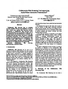
List of Figures 2.1
A simplified block diagram of the proposed JSIV delivery system. The client distortion estimation block, shown in gray, estimates client-side distortions in reconstructed frames without reconstructing them. . . . .
12
3.1
A block diagram of a basic image or video compression system. . . . . .
16
3.2
A simplified JPEG2000 encoder block diagram . . . . . . . . . . . . . .
18
3.3
A simple block diagram of a one-dimensional multi-resolution analysis/synthesis system. L0 is the incoming (original) signal. . . . . . . . .
3.4
21
A typical frequency response of each sub-band of a multi-resolution analysis system similar to the one shown in Figure 3.3 but with 3 levels of decomposition. ω is the angular frequency, and H(ω) is the overall filter response that is used in obtaining a given sub-band. . . . . . . . .
3.5
A typical lifting structure; analysis is shown on the left side and synthesis is shown on the right side. . . . . . . . . . . . . . . . . . . . . . . . . . .
3.6
22
Two-dimensional multi-resolution analysis system.
Top:
24
A block
diagram for the system. Bottom: Image decomposition into sub-bands. The superscripts v and h, as in hv0 and ↓h2, indicate that these operators are applied vertically and horizontally, respectively.
xi
. . . . . . . . . . .
25
3.7
A dead-zone quantizer with ξ = 0 and a dead-zone de-quantizer with δ =
1 2.
The upper part shows the centroids of the intervals; these are
the de-quantized values for a given index q. The lower part shows the quantization intervals; any value within a given interval is quantized to the index of that interval. . . . . . . . . . . . . . . . . . . . . . . . . . . 3.8
3.9
27
Each sub-band is partitioned into code-blocks. Each square, , represent one code-block. Gray blocks,
, represent one precinct.
. . . . . . . . .
Only the gray code-blocks,
, in the left-hand side are needed to
28
synthesize the window of interest (shown in grey) on the right-hand side.
32
3.10 A typical block diagram for a closed-loop predictive encoder. . . . . . .
33
3.11 A typical block diagram for a closed-loop predictive decoder. . . . . . .
34
3.12 Sequential prediction arrangement. Each rectangle represent one frame. Here, we have one I-frame followed by a number of P-frames. Arrows show prediction directions and the numbers at the top of the frames are frame indices. . . . . . . . . . . . . . . . . . . . . . . . . . . . . . . . . .
36
3.13 Hierarchical B-frames prediction arrangement. Two GOPs are shown for the case of K = 3. Solid black frames are I-frames. Darker gray frames have lower temporal rate. Arrows show prediction directions and the numbers at the top of the frames are indices. . . . . . . . . . . . . . . .
37
3.14 A block diagram for an example open-loop encoder. . . . . . . . . . . .
39
3.15 Motion compensated temporal filtering using the 5/3 wavelet. Frames lk−1 , lk , and lk+1 are temporally low-pass frames. Frames hk−1 and hk are the temporally high-pass frames.
. . . . . . . . . . . . . . . . . . .
41
3.16 Multi-level wavelet temporal filtering. Each level temporally decomposes the incoming frames in temporally low-pass frames and high-pass frames. L and H refers to the low-pass and high-pass paths; the subscript refers to the decomposition level.
. . . . . . . . . . . . . . . . . . . . . . . . .
xii
42
3.17 A typical block diagram for a scalable video encoder; the encoder employs an open-loop enhancement layer approach. . . . . . . . . . . . . . . . . .
43
3.18 A typical block diagram for a scalable video decoder; the decoder employs an open-loop enhancement layer approach. . . . . . . . . . . . . . . . . .
44
3.19 A block diagram for a Wyner-Ziv video encoder and decoder [29]. . . . .
49
4.1
A weighted acyclic directed graph (WADG), D, showing prediction relationship among various precincts with their corresponding scaling factors. The gray part of the graph is for possible precincts that are not used during discussions. . . . . . . . . . . . . . . . . . . . . . . . . . . .
4.2
58
An illustrative example showing how distortion propagates from one precinct to other precincts. The figure shows five precincts, each from one frame, that are indexed by the same π for a WOF composed of 5 consecutive frames. P1π is a reference precinct while each of the other precincts is predicted from the precinct before as indicated by the arrows. Underneath each precinct, we show the distortion contribution of that precinct. The gray area is the contribution of the distortion in precinct P3π to the other precincts in the WOF.
4.3
. . . . . . . . . . . . . . . . . .
59
A typical distortion-length convex hull for a precinct Pnπ , where each large white circle ( ) represents one quality layer. Also shown in the figure is π , the distortion associated with the predicted version of the precinct, D→n π π (0); the small black circles ( ) represent the modified < D∗n when D→n
convex hull.
. . . . . . . . . . . . . . . . . . . . . . . . . . . . . . . . .
xiii
63
4.4
Lack of embedding in JSIV. The first row shows two frames, f1 and f2 , of 60 × 60 pixel resolution compressed using JPEG2000 with 32 × 32 pixel code-blocks. The blocks in the middle of the second and third rows represent the number of quality layers inside each code-block of the DWT decomposition of each frame. Each square is one code-block and they are LL1 , HL1 , LH1 , and HH1 arranged from left to right, top to bottom. “P” indicates prediction. . . . . . . . . . . . . . . . . . . . . . . . . . . . . .
4.5
A comparison of the performance of various schemes for the “Speedway” sequence. . . . . . . . . . . . . . . . . . . . . . . . . . . . . . . . . . . .
4.6
76
The effect of code-block size on quality for the “Speedway” sequence when the “Sequential” prediction arrangement is employed. . . . . . . .
4.8
75
A comparison of the performance of various schemes for the “Professor” sequence. Note that the x-axis is in (kbit/frame). . . . . . . . . . . . . .
4.7
70
77
The effect of code-block size on quality for the “Professor” sequence when the “Sequential” prediction arrangement is employed. Note that the xaxis is in (kbit/frame). . . . . . . . . . . . . . . . . . . . . . . . . . . . .
4.9
78
A comparison between JSIV and SVC when the client is only interested in the retrieval of one frame. Note that the x-axis is in (Mb/frame). . .
79
4.10 A comparison of the performance of various schemes at full resolution and full/half temporal frame rate for the “Speedway” sequence. . . . . .
80
4.11 A comparison of the performance of various schemes at full resolution and full/half temporal frame rate for the “Professor” sequence. Note that the x-axis is in (kbit/frame). . . . . . . . . . . . . . . . . . . . . . .
81
4.12 A comparison of the performance of various schemes at half resolution and full/half temporal frame rate for the “Speedway” sequence. . . . . .
82
4.13 A comparison of the performance of various schemes at half resolution and full/half temporal frame rate for the “Professor” sequence. Note that the x-axis is in (kbit/frame). . . . . . . . . . . . . . . . . . . . . . .
xiv
83
4.14 A comparison between SVC and JSIV when the client is interested in only the left half of each frame of the “Speedway” sequence. SVC does not support such an option for pre-compressed sequences. . . . . . . . .
84
4.15 A comparison between SVC and JSIV when the client is interested in only the left half of each frame of the “Professor” sequence. SVC does not support such an option for pre-compressed sequences. Note that the x-axis is in (kbit/frame). . . . . . . . . . . . . . . . . . . . . . . . . . . .
85
4.16 A comparison among various methods when the client cache has one good quality reference frame (frame 9). . . . . . . . . . . . . . . . . . . . . . .
86
4.17 The original frame 17 of the “Speedway” sequence. . . . . . . . . . . . .
90
4.18 Frame 17 of the “Speedway” sequence when JSIV with the hierarchical prediction arrangement is employed. Frame 17 is an independent frame (an I-frame) in the hierarchical B-frame arrangement, as shown in Figure 3.13. . . . . . . . . . . . . . . . . . . . . . . . . . . . . . . . . . .
91
4.19 Frame 17 of the “Speedway” sequence when it is independently optimized. Rates are selected to be as close as possible to the rates used in Figure 4.18.
. . . . . . . . . . . . . . . . . . . . . . . . . . . . . . . . .
92
4.20 Frame 17 of the “Speedway” sequence when SVC is employed. Frame 17 is an independent frame (an I-frame) in the hierarchical B-frame arrangement, as shown in Figure 3.13. . . . . . . . . . . . . . . . . . . .
93
4.21 The original frame 23 of the “Speedway” sequence. . . . . . . . . . . . .
94
4.22 Frame 23 of the “Speedway” sequence when JSIV with the hierarchical prediction arrangement is employed. This frame is in the B2 position in the hierarchical B-frame arrangement, as shown in Figure 3.13. . . . . .
95
4.23 Frame 23 of the “Speedway” sequence when it is independently optimized. Rates are selected to be as close as possible to the rates used in Figure 4.22. . . . . . . . . . . . . . . . . . . . . . . . . . . . . . . . . . .
xv
96
4.24 Frame 23 of the “Speedway” sequence when SVC is employed. This frame is in the B2 position in the hierarchical B-frame arrangement, as shown in Figure 3.13. . . . . . . . . . . . . . . . . . . . . . . . . . . . . .
97
4.25 The original frame 12 of the “Professor” sequence. . . . . . . . . . . . .
98
4.26 Reconstructed frame 12 of the “Professor” sequence when JSIV with the hierarchical arrangement is employed. This frame is in the B3 position in the hierarchical B-frame arrangement, as shown in Figure 3.13. These images are resized to half their original size before including them in this document. . . . . . . . . . . . . . . . . . . . . . . . . . . . . . . . . . . .
99
4.27 Reconstructed frame 12 of the “Professor” sequence when it is independently optimized. Rates are selected to be as close as possible to the rates used in Figure 4.26. These images are resized to half their original size before including them in this document. . . . . . . . . . . . . . . . . 100 4.28 Reconstructed frame 12 of the “Professor” sequence when SVC is employed. This frame is in the B3 position in the hierarchical B-frame arrangement, as shown in Figure 3.13. These images are resized to half their original size before including them in this document. . . . . . . . . 101
xvi
5.1
Relation between the different partitions in this work.
2D-DWT
decomposes a given frame, fn , into sub-bands; a two-level decomposition is shown with sub-band labels that follow sub-band naming conventions. Each sub-band is partitioned into code-blocks, Cnβ ; in this figure, for example, each sub-band at the lower decomposition level, LL2 , HL2 , LH2 , and HH2 , has 4 code-blocks while, at the higher level, each has 16 code-blocks. Each sub-band is also partitioned into smaller blocks, known as grid blocks. A grid block, Gnγ , is shown as a small square; in the figure, each code-block has 16 grid blocks. A precinct, Pnπ , groups code-blocks that contribute to the same spatial region from three subbands, HLd , LHd , and HHd , at a given decomposition level, d; precincts for the LLD sub-band, where D is the number of decomposition level, contains code-blocks from that sub-band only. 5.2
. . . . . . . . . . . . . . 104
Distortion propagation from reference frames to predicted frames; here, frame fi is directly decoded, frame fj is at least partially predicted from fi , and frame fk is at least partially predicted predicted from fj .
The figure shows a two-level decomposition of each frame with
sub-band labels that follow sub-band naming conventions. The figure also shows code-blocks as squares; grid-blocks are not shown to reduce clutter. Decoded code-blocks are shown as ( ), predicted code-blocks as ( ). Arrows between fi and fj show distortion propagation from a given grid-block, Giγ , to many grid blocks in fj ; we approximate the distortion b →b
i j multiplied by the distortion in propagated along each arrow by GW(γ j)
Giγ . The dashed arrows between fj and fk represent possible distortion propagation that does not occur because the destination code-blocks in fk are replaced by directly decoded code-blocks.
xvii
. . . . . . . . . . . . . 105
5.3
(a) A typical WADG representing distortion propagation from reference grid blocks to predicted grid blocks. Each column represent one frame; frame fi is directly decoded, frame fj is predicted from fi , and frame fk is predicted from fj . Each node represents one grid block; an “∗” on the bottom-left side of a node indicates that the node is directly decoded rather than predicted. Each arrow represent distortion propagation with b →b
i j . (b) The converse of the WADG in (a). a distortion gain of GW(γ j)
Arrows indicate back-propagation of contribution weights from predicted frames to reference frames. 5.4
. . . . . . . . . . . . . . . . . . . . . . . . . 107
A typical distortion-length convex hull for a precinct Pnπ , where each large white circle ( ) represents one quality layer. Also shown in the π , figure is the distortion associated with predicted precinct samples, D→n π π (0); the small black circles ( ) represent the modified < D∗n when D→n
convex hull. 5.5
. . . . . . . . . . . . . . . . . . . . . . . . . . . . . . . . . 114
The effect of distortion propagation from a reference frame fr to a predicted frame fn when the 2D-DWT is employed. In general, all the sub-bands in fr contribute to the distortion in region Rn of frame fn . Most of these contributions, however, come from the projections of region Rn onto the sub-bands of fr , which are shown in gray in the 2D-DWT decomposition of fr ; here, we focus on one such region, Rr . Region Rr ← − r →bn encloses location W br→n (p) which corresponds to location p of Rn . . . 117
5.6
The server can potentially explore more than one prediction model for a given frame and select the most appropriate one. To do that the server π(γ)
γ (qn needs to store D∗n
π (q π ) for each frame, and q T,π , W ) and P∗n →n →n , n
M,γ π (q π ), q T,π , and W for each predictor. Only P∗n and D→n →n →n are delivered n
to the client. . . . . . . . . . . . . . . . . . . . . . . . . . . . . . . . . . 119 5.7
A comparison of the performance of various schemes for the “Crew” sequence. . . . . . . . . . . . . . . . . . . . . . . . . . . . . . . . . . . . 132
xviii
5.8
A comparison of the performance of various schemes for the “City” sequence. . . . . . . . . . . . . . . . . . . . . . . . . . . . . . . . . . . . 133
5.9
A comparison of the performance of various schemes for the “Aspen” sequence. Note that the x-axis is in (kbit/frame). . . . . . . . . . . . . . 134
5.10 The effect of code-block size on the quality of reconstructed video for the “Crew” sequence with hierarchical B-frame arrangement. . . . . . . . . 135 5.11 The effect of code-block size on the quality of reconstructed video for the “City” sequence with hierarchical B-frame arrangement. . . . . . . . . . 136 5.12 A demonstration of the flexibility of JSIV. A client can immediately utilize the availability of better motion vectors in improving the quality of reconstructed video. The figure shows the PSNR for the first 10 frames of the “Aspen” sequence; “Sequential” prediction arrangement is used here.137 5.13 A demonstration of the flexibility of JSIV. A client that browses the same section of a video will progressively get improved quality. The figure shows the PSNR for the first 10 frames of the “Aspen” sequence. “Sequential” prediction arrangement is used here. Each frame receives around 10.5 kBytes at each browsing session. . . . . . . . . . . . . . . . 138 5.14 Frame 13 of the “Crew” sequence. Frame 13 is in the B1 position in the hierarchical B-frame arrangement, as shown in Figure 3.13. . . . . . . . 145 5.15 Reconstructed frame 13 of the “Crew” sequence when JSIV with the hierarchical prediction arrangement is employed. Frame 13 is in the B1 position in the hierarchical B-frame arrangement, as shown in Figure 3.13.146 5.16 Reconstructed frame 13 of the “Crew” sequence when it is independently optimized. Rates are selected to be as close as possible to the rates used in Figure 5.15. . . . . . . . . . . . . . . . . . . . . . . . . . . . . . . . . 147 5.17 Reconstructed frame 13 of the “Crew” sequence when JSIV with the sequential prediction arrangement is employed. . . . . . . . . . . . . . . 148
xix
5.18 Reconstructed frame 13 of the “Crew” sequence when it is independently optimized. Rates are selected to be as close as possible to the rates used in Figure 5.17. . . . . . . . . . . . . . . . . . . . . . . . . . . . . . . . . 149 5.19 Frame 15 of the “City” sequence. Frame 15 is in the B2 position in the hierarchical B-frame arrangement, as shown in Figure 3.13. . . . . . . . 150 5.20 Reconstructed frame 15 of the “City” sequence when JSIV with the hierarchical prediction arrangement is employed. Frame 15 is in the B2 position in the hierarchical B-frame arrangement, as shown in Figure 3.13.151 5.21 Reconstructed frame 15 of the “City” sequence when it is independently optimized. Rates are selected to be as close as possible to the rates used in Figure 5.20. . . . . . . . . . . . . . . . . . . . . . . . . . . . . . . . . 152 5.22 Frame 14 of the “Aspen” sequence. Frame 14 is in the B3 position in the hierarchical B-frame arrangement, as shown in Figure 3.13. These images are spatially reduced by 2 before including them in this document.153 5.23 Reconstructed frame 14 of the “Aspen” sequence when JSIV with the hierarchical prediction arrangement is employed. Frame 14 is in the B3 position in the hierarchical B-frame arrangement, as shown in Figure 3.13. These images are resized to half their original size before including them in this document. . . . . . . . . . . . . . . . . . . . . . . 154 5.24 Reconstructed frame 14 of the “Aspen” sequence when it is independently optimized. Rates are selected to be as close as possible to the rates used in Figure 5.23. These images are resized to half their original size before including them in this document. . . . . . . . . . . . . . . . . . . . . . . 155
xx
List of Tables 3.1
The CDF 9/7 wavelet filters (or kernels) used in the JPEG2000 standard. 23
3.2
Lifting parameters for the CDF 9/7 wavelet transform. . . . . . . . . . .
4.1
A Comparison between different policies for the Speedway sequence. All results are in PSNR (dB). . . . . . . . . . . . . . . . . . . . . . . . . . .
4.2
68
Overheads in JSIV for the “Professor” sequence in hierarchical B-frame arrangement as a percentage of the overall rate. . . . . . . . . . . . . . .
5.1
68
A Comparison between different policies for the Professor sequence. All results are in PSNR (dB). . . . . . . . . . . . . . . . . . . . . . . . . . .
4.3
24
77
An example showing source sub-bands for each destination sub-band for 3 different significance thresholds, TS , when translational motion model is employed with CDF 9/7 irreversible wavelet transform and 5 levels of spatial decomposition. . . . . . . . . . . . . . . . . . . . . . . . . . . . . 121
5.2
Overheads in JSIV for the “City” sequence in sequential arrangement as a percentage of the overall rate. . . . . . . . . . . . . . . . . . . . . . . . 133
5.3
Overheads in JSIV for the “Aspen” sequence in hierarchical B-frames arrangement as a percentage of the overall rate. . . . . . . . . . . . . . . 135
5.4
A Comparison between different policies for the “City” sequence. Results are in PSNR (dB). . . . . . . . . . . . . . . . . . . . . . . . . . . . . . . 140
5.5
A Comparison between different policies for the “Aspen” sequence. Results are in PSNR (dB). . . . . . . . . . . . . . . . . . . . . . . . . . . 140 xxi
List of Symbols Symbol
Meaning
fn
A frame index by n
grn
Position-independent scaling factor used in predicting fn from fr
f→n
A predictor for fn
fr→n
A predictor for fn obtained from fr
Wa→b (·)
The motion compensation operator mapping fa to fb
Fs
A window of frames (WOF) indexed by s
Cnβ
A code-block indexed by β from frame fn
C˚nβ
Full-quality samples for code-block Cnβ
Dnβ
The distortion associated with Cnβ
qnβ
The number of quality layers in Cnβ
� � � β� �qn �
The number of bytes in qnβ quality layers
Gb β
The energy gain of sub-band b to which code-block β belongs
Q
The maximum number of quality layers
β β or C∗n (qnβ ) C∗n
De-quantized samples for code-block Cnβ
β β D∗n or D∗n (qnβ )
β β The distortion associated with C∗n or C∗n (qnβ )
β C→n
Predicted samples for code-block Cnβ
β Cr→n
Predicted samples for code-block Cnβ obtained from fr
xxii
β D→n
β The distortion associated with C→n
β Dr→n
β The distortion associated with Cr→n
M,β D→n
β The motion distortion component in D→n
Q,β D→n
β The quantization distortion component in D→n
Q,β Dr→n
β The quantization distortion component in Dr→n
Pnπ
A precinct indexed by π from frame fn
Dnπ
The distortion associated with Pnπ
qnπ
The number of quality layers in Pnπ
qnp,π
qnπ at epoch p
T,π q→n
π The quality layer threshold associated with P→n
π or P π (q π ) P∗n ∗n n
De-quantized samples for precinct Pnπ
π or D π (q π ) D∗n ∗n n
π The distortion associated with P∗n
π P→n
Predicted samples for precinct Pnπ
π Pr→n
Predicted samples for precinct Pnπ obtained from fr
π D→n
π The distortion associated with P→n
π Dr→n
π The distortion associated with Pr→n
M,π D→n
π The motion distortion component in D→n
Q,π D→n
π The quantization distortion component in D→n
Q,π Dr→n
π The quantization distortion component in Dr→n
Gnγ
A grid-block indexed by γ from frame fn
Dnγ
The distortion associated with Gnγ
qn
π(γ)
The number of quality layers associated with Gnγ
Gb γ
The energy gain of sub-band b to which grid block γ belongs π(γ)
γ γ or G∗n (qn G∗n
)
π(γ)
γ γ D∗n or D∗n (qn
)
De-quantized samples for grid block Gnγ π The distortion associated with G∗n
xxiii
γ G→n
Predicted samples for grid block Gnγ
γ Gr→n
Predicted samples for grid block Gnγ obtained from fr
γ D→n
γ The distortion associated with G→n
γ Dr→n
γ The distortion associated with Gr→n
M,γ D→n
γ The motion distortion component in D→n
A,γ D→n
γ The attributed distortion component in D→n
A,γ Dr→n
γ The attributed distortion component in Dr→n
π (q π ) ˆ ∗n D n π ˆ →n D
π (q π ) Weighted (effective) precinct distortion associated with P∗n n π Weighted (effective) precinct distortion associated with P→n
χπn
A hidden state variable associated with Pnπ
π(γ)
A hidden state variable associated with Gnγ
θnπ
The additional contribution weight associated with Pnπ
Ψo
The rate-distortion optimization pass
Ψw
The contribution weight pass
χn
λ λπn or λπn (q)
The Lagrangian parameter π The distortion-length slope associated with P∗n
ˆ π (q) λ n
π Weighted (effective) distortion-length slope associated with P∗n
A(x)
The antecedents of x; the set of things that contributes to x
S(y)
The succedents of y; the set of things that receives contributions from y
b →b
i j GW(p)
Position-dependent distortion gain from Giγ of sub-band bi in fi to point p in Gjγ of sub-band bj in fj
¯ bi →bj G W(p)
b →b
i j The average of GW(p) around point p due to the possibly
many phases of p b →b
i j GW(γ j)
Position-dependent (i.e. grid block dependent) distortion gain
xxiv
← − r →bn W br→n (·) − → r →bn W br→n (·)
from Giγ of sub-band bi in fi to Gjγ of sub-band bj in fj The operator that maps locations in sub-band bn of fn back to locations in sub-band br of fr , according to the motion model The operator that maps locations in sub-band br of fr to locations in sub-band bn of fn , according to the motion model
xxv
Chapter 1
Introduction 1.1
Motivation
Digital video nowadays comes in an ever increasing resolution and bit depth. Today’s consumer video is captured in high definition (HD) with a resolution ranging from 1280× 720 pixels to 1920×1080 pixels. Digital cinema employs a resolution of up to 4096×2160 pixels [56]. Even higher resolutions are under consideration for future TV broadcasting such as the Ultrahigh-Definition Television [62] (also known as Super Hi-Vision) with a resolution of 7680 × 4320 pixels, and for military surveillance applications such as the ARGUS-IS [32] system with a resolution of 2.3 Gigapixels. These higher resolutions are also accompanied by higher bit depth; for example, digital cinema employs 12 bits per color component [56], and possibly even more spectral components if we take into consideration that surveillance footage can also be captured in infra-red, for example. Most commonly available digital video playback systems, on the other hand, come with a limited resolution; these devices can range from mobile phones with small and low resolution screens to an LCD display with HD resolution. Obviously, we need a mechanism that allows us to view all or part of such a high-resolution multi-component video on our playback devices taking into consideration the available bandwidth, the device’s playback resolution and processing power, as well as the client interest.
1
Chapter 1. Introduction To this end, we need to encode the original video sequence in a scalable and accessible way; moreover, we need an interactive protocol that allows us to remotely leverage the scalability and accessibility options provided by the encoded sequence. For still images, the JPEG2000 Interactive Protocol (JPIP) [42, 100] leverages the scalability and accessibility options of the JPEG2000 format and provides many of the desirable features of scalable interactive browsing. These include resolution scalability, progressive refinement (or quality scalability), spatial random access, and highly efficient compression. JPIP also supports interactive browsing of Motion-JPEG20001 , although we note that Motion-JPEG2000 content does not involve any exploitation of inter-frame redundancy. This absence of inter-frame redundancy exploitation can have a significant negative impact on video coding efficiency. For video sequences, interactive browsing has traditionally been limited to pause and random access to a predetermined set of access points. This limitation is a result of employing standard video compression techniques, such as MPEG-1 through MPEG-4 and H.261 through H.264, that can, at best, provide limited scalability and accessibility options. This limited interactivity as well as other issues motivated research in scalable video coding, which can provide considerably better interactivity and solve some of the existing problems in video storage and streaming. Research in the area has produced some promising results [60, 75] and recently (in 2007) a scalable video coding (SVC) extension to H.264/AVC [37, 86] has been approved within the ISO working group known as MPEG, in order to provide improved scalability options. Despite these improved options, the encoder still imposes restrictions on the encoded stream that limit accessibility, which in turn, limit interactivity. For example, in order to deliver a given frame to the client, the server has to send enough data from the group of pictures (GOP) that contains this frame, possibly the whole GOP, and the client has to decode potentially many frames in order to invert the motion compensated transform 1
Motion-JPEG2000 [41] is a video file format based on JPEG2000. The file contains some video timing information, and each frame is stored independently in its own code-stream.
2
Chapter 1. Introduction used during compression and extract the desired frame. More examples are provided in the following chapters.
1.2
Problem Statement
The aim of this work is to propose a novel paradigm that provides considerably better interactivity for video browsing. The interactivity options sought include spatial resolution scalability, quality scalability (or progressive refinement), frame rate (or temporal) scalability, and spatial and temporal random accessibility. The scalability sought can also involve a combination of these scalability options; for example, a client might be interested in half frame rate, half resolution version of the video sequence at reduced quality. An integral part of the proposed paradigm is the capability of the client to utilize its cache contents in a useful way to improve the quality of reconstructed video; it is possible that the client has more or less data than what the server is aware of. The difference occurs, for example, when data is lost or when the client is browsing the same media a second time, possibly communicating with a different server that is unaware of the client’s cache. This requires a server policy that is loosely-coupled to the client policy; such a policy allows the client to make its own decisions independent of the server decisions. The above objectives are necessary for a typical remote interactive browsing of video (for example, surveillance footage). In such a scenario, a remote client usually monitors a low-resolution version of the whole scene, possibly at a reduced temporal rate, as this provides the interactive user with sufficient details to identify any regions of interest. To have a more detailed look at any of these interesting regions, the interactive user changes his or her window of interest to that region, and starts monitoring it. It is also possible that the client examines the same video region (a number of consecutive frames with the same region of interest) for a few times to make sense of what he/she is seeing; it is natural to assume that he/she expects the quality of that region to improve 3
Chapter 1. Introduction as he/she spends more time on it.
1.3
Our Contribution
The original contribution of this work is in the proposed paradigm, its philosophy, and the mechanisms developed for a realistic implementation. For the conceptual aspects and the philosophy behind them, our contributions include: • The whole concept behind JSIV and its philosophy. • The concept of using prediction to exploit temporal redundancy within the context of JPEG2000 and interactive video browsing. Prediction in this case involves motion compensation and conditional replenishment. • The use of intra-coded precincts rather than residuals to update predicted frames. This has a negative impact on the quality of reconstructed video, but it relieves us from closed-loop prediction problems, such as drifting between the client and server states, and enables the use of loosely-coupled client and server policies. • The concept of not committing to a prediction policy, but rather selecting the most appropriate policy at serve-time. Not committing to a prediction policy with the aforementioned loosely-coupled policies and the use of only intra-coded precincts enable the client to make decision independently of the server. This independence allows the client to better utilize its cache contents. Our contributions towards a realistic implementation of a JSIV system include: • Casting the general JSIV problem as a Lagrange-style rate-distortion optimization problem, solving this problem using a two-pass iterative approach, and showing that this iterative approach converges. • The particular loosely-coupled client and server policies introduced in Chapters 4 and 5 that make a real implementation of the system possible. Each chapter 4
Chapter 1. Introduction employs slightly different policies that are more useful for the case investigated in that chapter. • The approximations introduced to make a real-time implementation possible. These approximations reduces the amount of needed calculations considerably without introducing major reduction in quality. • The concept of sending side-information in an additional image component. This allows us to benefit from the options of JPIP protocol without any changes to the protocol itself. Finally, another contribution is in demonstrating the efficacy of a realistic JSIV system in a wide variety of scenarios and test cases.
1.3.1
Publications
The following publications have emanated from this thesis work and related research: Journal Papers • A.T. Naman and D. Taubman.
JPEG2000-Based Scalable Interactive Video
(JSIV). Image Processing, IEEE Transactions on, Volume 20, Issue 5, pages 1435 - 1449, May 2011, http://dx.doi.org/10.1109/TIP.2010.2093905. • A.T. Naman and D. Taubman.
JPEG2000-Based Scalable Interactive Video
(JSIV) with Motion Compensation. Image Processing, IEEE Transactions on, available in early access section, should be in September 2011 issue, http: //dx.doi.org/10.1109/TIP.2011.2126588. Conference Papers • A.T. Naman and D. Taubman. A Novel Paradigm for Optimized Scalable Video Transmission Based on JPEG2000 with Motion. Proc. IEEE Int. Conf. Image Proc. 2007, pages V-93 - V-96, September 2007. 5
Chapter 1. Introduction • A.T. Naman and D. Taubman. Optimized Scalable Video Transmission Based on Conditional Replenishment of JPEG2000 Code-blocks with Motion Compensation. MV ’07: Proceedings of the International Workshop on Workshop on Mobile Video, pages 43-48, September 2007. • A.T. Naman and D. Taubman. Distortion Estimation for Optimized Delivery of JPEG2000 Compressed Video with Motion. IEEE 10th Workshop on Multimedia Signal Processing, 2008, MMSP 2008, pages 433-438, October 2008. • A.T. Naman and D. Taubman. Rate-Distortion Optimized Delivery of JPEG2000 Compressed Video with Hierarchical Motion Side Information. Proc. IEEE Int. Conf. Image Proc. 2008, pages 2312-2315, October 2008. • A.T. Naman and D. Taubman. Rate-Distortion Optimized JPEG2000-Based Scalable Interactive Video (JSIV) with Motion and Quantization Bin SideInformation. Proc. IEEE Int. Conf. Image Proc. 2009, pages 3081-3084, November 2009. • A.T. Naman and D. Taubman. Predictor Selection Using Quantization Intervals in JPEG2000-Based Scalable Interactive Video (JSIV). Proc. IEEE Int. Conf. Image Proc. 2010, pages 2897-2900, September 2010.
1.4
Outline of The Thesis
The rest of the thesis is arranged as follows. Chapter 2 introduces the main concepts behind the JPEG2000-Based Scalable Interactive Video (JSIV) paradigm. Chapter 3 contains the necessary background material needed for the rest of the thesis. We start by giving a simplified overview of scalable image coding with emphasis on the JPEG2000 coding scheme and its relevant aspects. Then, we discuss predictive video coding schemes, highlighting the interactivity options they provide and
6
Chapter 1. Introduction underlining their weaknesses and limitations that impact scalability and accessibility. We also discuss the general open-loop video coding systems that employ spatiotemporal transforms and highlight the effect of the temporal transform on accessibility. Additionally, we discuss the basic concepts of scalable motion coding, highlighting its advantages, and distributed video coding, exploring its relation to JSIV. This is followed by a simplified overview of a couple of interactive protocols that are used for still image and video delivery over the Internet with emphasis on JPEG2000 Interactive Protocol (JPIP). We conclude this chapter by discussing some recent research in interactive video browsing. Chapter 4 discusses the case of JSIV that employs prediction without motion compensation. To this end, we start by introducing unrealistic client and server policies, namely “oracle” policies, that enables us to present the general JSIV optimization problem. We solve this problem by utilizing a two-pass iterative approach and we show that this approach converges under the assumptions made in the derivation of the optimization problem. The unrealistic policies are then revised with realistic ones. For real-time implementation, we introduce approximations that significantly reduce calculations with little or no impact on the quality of reconstructed video. We conclude the chapter with experimental results and comparisons to other coding schemes that span many of the interesting usage scenarios. Chapter 5 discusses JSIV when motion compensation is utilized in prediction. We follow a similar approach to that of Chapter 4; we start with “oracle” policies which enables us to solve the JSIV optimization problem, but we highlight the difference to the earlier case. Then, we revise these policies with realistic ones. The main contribution of this chapter is in exploring the effect of motion compensation on JSIV. We conclude the chapter by presenting some experimental results for JSIV’s performance and compare them to alternate coding schemes highlighting JSIV’s advantage in a couple of usage scenarios. Finally, Chapter 6 concludes the thesis and discusses possible areas of further
7
Chapter 1. Introduction research. While Chapter 3 is mostly literature survey, Chapters 2, 4 and 5 represent our original contribution.
8
Chapter 2
Introduction to JPEG2000-Based Scalable Interactive Video (JSIV) At this stage, we find it more convenient to present the proposed JPEG2000Based Scalable Interactive Video (JSIV), as this would put the following chapters in perspective. In this chapter, therefore, we present the main concepts behind the JSIV paradigm. We also discuss the applications that can benefit from this paradigm. To provide better flexibility, scalability, and interactivity options for video streaming compared to existing practices, we propose JPEG2000-Based Scalable Interactive Video (JSIV). JSIV relies on: • JPEG2000 to independently compress the individual frames of the video sequence and provide for quality and spatial resolution scalability as well as random accessibility. • Prediction, with or without motion compensation, and conditional replenishment of JPEG2000 code-blocks to exploit temporal redundancy. • Loosely-coupled server and client policies. The server policy aims to select the 9
Chapter 2. Introduction to JPEG2000-Based Scalable Interactive Video best number of quality layers for each precinct it serves and the client policy attempts to produce the best possible reconstructed frames from the data which the client has. Each of these policies may evolve separately without breaking the communication paradigm. The philosophy behind the loosely-coupled client and server policies of JSIV is that the client should not explicitly drive the server’s behaviour (e.g., it should not request the delivery of specific code-block bit-streams) and the server should not explicitly drive the client’s behaviour (e.g. it should not tell the client how to synthesize each frame from the delivered content). Instead, the client poses high level requests to the server (e.g., region of interest, playback resolution/frame-rate, etc.) and the server replies with portions of code-block bit-streams which it believes to be helpful in satisfying the client’s declared interests. We postulate that if both the client and the server are intelligent enough to make reasonable decisions, then the decisions made by the server are likely to have the expected impact on the decisions made by the client. For example, if the server sends a reasonable amount of data from a particular code-block bit-stream, judging this to be beneficial to the client, then a reasonable client policy is likely to use the supplied bit-stream rather than predict the code-block in question from neighbouring frames. The server may send motion information wherever it thinks that this information is useful in improving prediction. Motion information may be augmented with additional side information to help the client resolve highly ambiguous situations1 , but this side information should be expressed in a form which is independent of the state of the client-server interaction so that it describes properties of the source which are always true. There are many advantages to such an approach. One example is when the client has some data that the server is unaware of; for instance, the client might have obtained that data from a previous browsing session or from a different server or possibly a proxy. 1
For example, in the absence of any data for some code-block, it is not at all clear whether the client should synthesize the frame using zeros or predicted samples for that code-block.
10
Chapter 2. Introduction to JPEG2000-Based Scalable Interactive Video In this case the client uses its knowledge of the stream and its properties to consider both its cache content and the newly received data in order to select the options that, it believes, achieve the best possible quality. There is no need to worry about drifting between the client state and the server state, since the client makes its decisions based on properties of the stream which are always true. Other examples arise in the case where a client has less data than the server expects, for example due to data loss. In such cases, the client uses the knowledge it has about the stream and its properties to conceal any missing data. We move our attention to the simplified block diagram of a JSIV system depicted in Figure 2.1; the system has three basic entities: the preprocessing stage, the server, and the client. The preprocessing stage is responsible for compressing each frame independently of the other frames into the JPEG2000 format and preparing sideinformation for these frames. The side information can include distortion-length slope tables, motion information, motion distortions, and any other side information that might be required during media serving. Side-information can either be generated offline for pre-recorded media or in real-time for live media. Many of these operations are independent of each other and can be easily delegated to one or more machines in a content delivery network. The server is composed of two main sub-blocks: the client distortion estimation block (CDEB) and the rate-distortion optimization block (RDOB). The CDEB attempts to model distortions in each code-block or each precinct of each frame, based on its knowledge about transmitted information and an assumed client policy. This model can also be adapted to reflect knowledge of network conditions, client browsing preferences and client browsing cache.
It is sufficient for this block to generate approximate
estimates of distortions, and therefore it does not have to actually reconstruct the client’s view. The RDOB performs Lagrangian-style rate-distortion optimization to decide the number of quality layers to be sent for each precinct of each frame, which can be
11
12
Cache Model
Client Policy
Server Policy
Server
2D 2D-DWT 2 D-DW DDWT WT Ana An nal aly ysi sis Analysis
Motion M Mo otiion ot on Co C omp mpe pen ensa sat ati tio on Compensation
22D-DWT 2D D-D D-DW DWT WT Sy S ynt yn nth hes he esi siss Synthesis
Cood Code-block C ode dee-b -bl bloock Selection S ele lec ect ctiioon on
Rate-Distortion Optimization
High-Level Requests
Client
Motion Compensation
2D-DWT Analysis
Code-block Selection
Reconstructed Video
2D-DWT Synthesis
Cache Model
Client Policy
Figure 2.1: A simplified block diagram of the proposed JSIV delivery system. The client distortion estimation block, shown in gray, estimates client-side distortions in reconstructed frames without reconstructing them.
Preprocessing
Video Content
Preprocessing Stage JPEG2000 Compression, Motion Estimation, Some Statistics
Motion-information
Side-information
JPIP
Side-information
Client Distortion Estimation
Optimal Selection of Code-blocks
Motion-information
Code-blocks
Chapter 2. Introduction to JPEG2000-Based Scalable Interactive Video
Chapter 2. Introduction to JPEG2000-Based Scalable Interactive Video zero. It also decides on any side-information needed by the client to best exploit the frame data. All the decisions made by the RDOB take into consideration the estimated distortion provided by the CDEB. The server communicates with the client employing only JPIP [42, 100]; JSIV stores side-information in additional components within each frame, conceptually known as meta-components or meta-images. This allows the use of JPIP without any modifications to send both code-block data and side-information; a standard JPIP client communicating with a JSIV server can simply ignore these extra components. The client receives compressed code-block bit-streams and side information. Using this information, aided by a client policy, the client selects the source of data to use for each code-block. In particular, the client has the option to decode an available codeblock bit-stream directly or to predict the code-block from nearby frames (possibly having much higher quality). The flexibility and accessibility of JSIV is the result of not committing to any predetermined temporal prediction policy. Thus, the server is free to change its policy on the fly and during serve time to respond to changes in client requirements or network conditions. JSIV departs from traditional predictive coding schemes in that side-information in JSIV is only a guide which helps the client make sound decisions while in traditional video compression schemes it totally dictates the client prediction modes, prediction reference frames, and any other client operation modes. Also, JSIV always sends intracoded frame pieces and never uses residual data. The use of actual data instead of residual data incurs an encoding loss, but at the same time, enables the client to make decisions independently of the server and avoid the possibility of drift between server and client states. This independence enables the client to use its cache more effectively and possibly use information obtained from other servers or proxies.
13
Chapter 2. Introduction to JPEG2000-Based Scalable Interactive Video
2.1
Applications Where JSIV is Advantageous
Remote browsing of high-resolution surveillance video is one application where JSIV can provide an improved browsing experience compared to current video coding standards. Usually for such video sequences, most of the changes happen in certain regions, and the background occupies a good percentage of the frames, with little or no changes. For such cases, JSIV works better than conventional JPIP since it effectively reduces to an optimized conditional replenishment scheme while JPIP by itself needs to transmit the full content of each frame. We have described a typical browsing scenario for surveillance footage in Section 1.2; in such a scenario, the client usually proceeds from low-resolution version of the whole scene to a more detailed look at a window of interest. For monitoring a window of interest, JSIV works favourably compared to existing coding standards, as these do not support retrieval of an arbitrary window of interest from a pre-compressed video sequence. Other advantages of JSIV for surveillance video browsing over existing paradigms include the capability of backward playback, reduced temporal rate playback, and lossless retrieval of frames or regions of interest in frames. For lossy transmission environments, the server does not need to retransmit lost packets, instead it can adapt by adjusting its delivery policy for future frames alone. For video browsing, both the client and the server can easily and dynamically change from video playback mode to individual frame browsing mode and any data in the client’s cache is readily available for the reconstruction of individual frames. For clients with limited processing capabilities, the server can adapt its policy by reducing frame rate, reducing resolution, or by focusing on the client’s window of interest. There is also no need for the server to use the same motion model with every client, which provides more options to handle clients with diverse needs and channel conditions.
14
Chapter 3
Scalable Interactive Image and Video Browsing This chapter briefly describes some of the basic concepts employed in any image or video compression system. It also explores some of the more sophisticated approaches used in some practical image and video compression systems. We start by introducing a block diagram of a basic image or video compression system. Then, we discuss the JPEG2000 image compression standard, closed-loop predictive video coding, open-loop video coding, scalable motion coding, and distributed video coding. This is followed by a brief discussion of some of the protocols used in interactive image and video delivery. We conclude this chapter by a brief overview of some recent research in the area of interactive video delivery. The main focus of this chapter is the interactivity available to video browsing; that is, the scalability and accessibility options provided by the reviewed approach.
3.1
A Basic Compression System
The purpose of an image or video compression algorithm is to represent that image or video with the smallest possible amount of data for a given quality. To this end,
15
Chapter 3. Scalable Interactive Image and Video Browsing the majority of image and video compression algorithms employ, in general, a block diagram similar to that shown in Figure 3.1; the building blocks of such a system are: transformation, quantization, and source coding. Although we present these blocks as separate entities, they are, in reality, closely related; to achieve optimal results, the design of one stage should take into consideration the output of the earlier stage. For example, the code-block arithmetic coder of the JPEG2000 standard uses different context rules for different sub-bands; these rules take into consideration that the HL sub-band tends to have vertical edges and the LH sub-band tends to have horizontal edges. Image or Video
Transformation
Coefficients
Quantization
Quantized Coefficients
Source Coding
Compressed Image or Video
Figure 3.1: A block diagram of a basic image or video compression system.
3.1.1
Transformation
The purpose of transformation is to remove or considerably reduce any dependency between data values; that is, to decorrelate these values. This true for still images and for video sequences, where decorrelation is performed along both spatial and temporal dimensions. For colour components, many compression techniques employ a colour decorrelation transform, as the colour components in their original colour space can be highly correlated; for example, most compression algorithms convert from the RGB colour space representation to YUV. Then, each decorrlated component undergoes further spatio-temporal decorrelation transformation. Within one component (or a single-component image), the transformation maps the samples of that component into a set of coefficients, which are then quantized and coded. This transformation process can be interpreted as a signal projection; the original signal is viewed as a multidimensional vector that is projected into a multidimensional basis. A characteristic of a good transform (or a good basis) is that it is able to collect most 16
Chapter 3. Scalable Interactive Image and Video Browsing of the image energy into a small number of significant coefficients for a wide variety of images; this is known as energy compaction. The other coefficients are of small magnitude and can be coarsely quantized (or totally ignored) with only little distortion to the original image [31, 106].
3.1.2
Quantization
Quantization involves dividing the range of the coefficients obtained from the transformation step into intervals. Generally, each interval is mapped into its own symbol1 (or sometimes interpreted as an event) that is then coded (Section 3.1.3). The entropy of these symbols or events is smaller than the entropy of the original coefficients by virtue of mapping a whole range of symbols into a single symbol. Thus, quantization is irreversible and it is the step where information loss occurs, since the transformation step usually employs a reversible transform. In general, the distortion introduced by quantization and the amount of data needed to encode the quantized coefficients are bound by the rate-distortion theory [9]; the ratedistortion theory is not an individual theory but rather a group of theories and results that are collectively known as the rate-distortion theory. This theory sets a bound on the minimum required rate subject to source statistics and acceptable distortion, or conversely, a bound on achievable minimum distortion subject to source statistics and available data rate.
3.1.3
Source Coding
Source coding aims at representing the symbols (or events) obtained from the quantization step in an invertible way using the least number of bits possible. The amount of data needed to represent these symbols is bound by Shannon’s noiseless source coding theorem [89]. Specifically, the average number of bits needed to represent 1
There are special cases where each interval is mapped into more than one symbol such as in distributed video coding.
17
Chapter 3. Scalable Interactive Image and Video Browsing these symbols (or events) is no less than the entropy of these symbols2 . To achieve maximum coding efficiency, the encoder must adapt to the statistics of the symbols being encoded; many existing source coding schemes follow this approach and employ adaptive codes with dynamic source statistics estimation. Good modelling of the source is an essential part of this process, and, in many cases, it is important to consider the context in which these symbols or events occur.
3.2
JPEG2000 Image Coding Standard
JPEG2000 is considered the successor to the JPEG still image coding standard; however, the two standards are considerably different and therefore JPEG2000 is backward incompatible with JPEG. JPEG2000 provides many desirable features such as improved coding efficiency and progressive lossy to lossless performance within a single data stream, but the more interesting features to this work are spatial-resolution scalability, progressive refinement (or quality scalability), and spatial accessibility. Original image
Colour Transform
Discrete Wavelet Transform
Quantization
Tier 1 (Arithmetic Coding)
Tier 2 (Assignment)
Compressed image
Embedded Coding
Figure 3.2: A simplified JPEG2000 encoder block diagram Figure 3.2 shows a simplified block diagram of a JPEG2000 encoder. The first block performs a colour transform if it is needed. This is followed by two-dimensional discrete wavelet transform (2D-DWT). The transformed samples are then quantized before going through the embedded block coding with optimized truncation (EBCOT). The following is a more detailed description of each stage with focus on the irreversible path of Part 1 of the standard [39]. 2
It is widely accepted that this statement is, in general, true; however, under special conditions, it is possible to find codes that achieve below-entropy code rate for the case of some constrained sources with memory when the overall compressed data length is known [19].
18
Chapter 3. Scalable Interactive Image and Video Browsing
3.2.1
Colour Transform
The first step in the encoder is, actually, to offset any bias that the input samples have [81, 103]; that is, convert the unsigned samples with a range of [0, 2B ) to signed values with a range of [−2B−1 , 2B−1 ), where B is the number of bits per sample per component of the input image, by subtracting 2B−1 . This step is followed by colour transform if the input samples are in RGB space. The colour transform is employed to exploit the redundancy that exist between the colour components in the RGB space and to represent the information in a space that is more suitable for quantization, since it corresponds better to the Human Visual System (HVS) [17]. Part 1 of the JPEG2000 standard [39] specifies two types of colour transforms, the reversible colour transform (RCT) used for the reversible path, and the irreversible colour transform (ICT) used for the irreversible path. More details about these two paths are given in the next subsections. The main difference between RCT and ICT is that the former can be reconstructed exactly with finite integer precision, whereas the latter uses floating-point arithmetic and there is no guarantee on exact reconstruction of the original values when integer representation is used, especially when rounding or clipping is employed as in the case of integer-valued image samples. The ICT transform applies a piece-wise linear operator on the RGB components, denoted by xR , xG , and xB , to produced the transformed components, denoted by xY , xCb , and xCr ; this operator is given by x Y � αR x R + α G x G + α B x B 0.5 (xB − xY ) 1 − αB 0.5 � (xR − xY ) 1 − αR
x Cb � x Cr
(3.1)
where αR � 0.299, αG � 0.587, αB � 0.114 [103]. This operator should be treated as a definition; all the other related conversions should be derived from this equation with these parameters. We leave the definition of the RCT to the reader as it is irrelevant 19
Chapter 3. Scalable Interactive Image and Video Browsing to our work. Part 2 of the standard [40, 81] allows for user-defined offsets and colour transforms.
3.2.2
Discrete Wavelet Transform
The Discrete Wavelet Transform (DWT) provides the multi-resolution analysis [44, 55] required for the resolution scalability feature of the JPEG2000 format. Unlike the Fourier transform which provides good frequency resolution but no spatial information, the DWT provides simultaneous space-frequency analysis that has both spatial and frequency information. Compared to the block-based transforms of Section 3.3, the DWT has the advantage that it is an overlapping transform and therefore does not suffer from artefacts at block boundaries. Multi-resolution models are known to work better in describing the HVS [54]. This might explain why JPEG2000 performs better in subjective tests [103]. Another way of explaining the suitability of DWT for image compression is the fact that most of the image energy is usually concentrated in low-frequency information while highfrequency information is often clustered around the edges only. For this reason, the multi-resolution analysis provided by the DWT is ideal in these situations [110]. The Laplacian pyramid [11] is another multi-resolution analysis technique. For image compression, the advantage of the DWT over the Laplacian pyramid technique is that the number of samples that need to be compressed and stored is the same as the original image whereas in the Laplacian pyramid case, that number is approximately 4/3 times the number of samples in the original image. However, the need for perfect reconstruction in the DWT case imposes certain restrictions on the filters that cause aliasing in reconstructed images at reduced spatial resolutions; there are no such restrictions in the case of the Laplacian pyramid, and therefore filters in this case can be designed to produce alias-free images at reduced spatial resolution. The multi-resolution analysis decomposes the incoming signal into a set of bandlimited sub-bands which are then quantized and coded. For this reason, the process
20
Chapter 3. Scalable Interactive Image and Video Browsing described here is also known as sub-band coding. The simultaneous space-frequency multi-resolution analysis is achieved with polyphase decomposition of the incoming signal with properly designed filters. As such, the DWT is defined by two sets of filters; the first set is known as the analysis filters and denoted by hi [n] and the second is known as synthesis filters and is denoted by gi [n]. Perfect reconstruction imposes certain restrictions on the filters and therefore these filters are closely related. Generally, there are M analysis filters and M synthesis filters; the analysis filters transform the incoming signal into M sub-bands. We focus here on the case of two-channel transforms (M = 2) since it is the only available option in Part 1 of the JPEG2000 format. Figure 3.3 shows a simple block diagram of a one-dimensional multi-resolution analysis/synthesis system that utilizes a two-channel DWT; h0 has predominantly lowpass characteristics and h1 has predominantly high-pass characteristics. On the analysis side, the incoming signal is filtered by h0 and h1 and sub-sampled by 2, as shown in Figure 3.3, to produce L1 and H1 , respectively. Then, L1 undergoes a similar process to produce L2 and H2 . This process can be repeated again on L2 to further analyse it into L3 and H3 . A typical frequency response for such a system is shown in Figure 3.4. On the synthesis side, L2 and H2 are up-sampled by 2 then filtered by g0 and g1 , respectively. These two signals are then added to produce L1 . Then, both L1 and H1 undergo a similar process to reconstruct the original signal. Level 1
Level 2 h0
h0
↓2
L2
↑2
Level 1
g0 L1
h1 ↓2
L2
L1
L0 h1
↓2
Level 2
↓2
H2
H2
↑2
H1
g0 L0
g1 H1
Analysis
↑2 ↑2
g1
Synthesis
Keys: ↑ 2 is up-sample by 2, ↓ 2 is sub-sample by 2.
Figure 3.3: A simple block diagram of a one-dimensional multi-resolution analysis/synthesis system. L0 is the incoming (original) signal. 21
Chapter 3. Scalable Interactive Image and Video Browsing |H(ω)|2 L3 0
H3 π/8
H2 π/4
H1 π/2
π
ω
Figure 3.4: A typical frequency response of each sub-band of a multi-resolution analysis system similar to the one shown in Figure 3.3 but with 3 levels of decomposition. ω is the angular frequency, and H(ω) is the overall filter response that is used in obtaining a given sub-band. Perfect reconstruction requires that [31, 106]
H0 (z)G0 (z) + H1 (z)G1 (z) = 2;
(3.2a)
H0 (−z)G0 (z) + H1 (−z)G1 (z) = 0;
(3.2b)
where H0 (z), H1 (z), G0 (z), G1 (z) are the z-transforms of h0 [n], h1 [n], g0 [n], g1 [n], respectively. For the purpose of image compression, these filters should have a linear phase (or equivalently constant group delay) because the HVS is sensitive to phase distortions, especially around the edges [104]. As such, only finite impulse response (FIR) filters with symmetric coefficients are allowed. Thus, the discussion here is only for symmetric biorthogonal wavelets. Extensive treatment of the theory of wavelets and sub-band transforms can be found in [20, 92, 104], and biorthogonal wavelets are discussed in [18, 48, 51, 76, 104]. Part 1 of the JPEG2000 standard defines two biorthogonal wavelet filters, the CohenDaubechies-Feauveau (CDF) 9/7 wavelet for the irreversible path, and the Spline 5/3 wavelet for the reversible path. Table 3.1 gives these filter coefficients for the CDF 9/7 wavelet filters. The wavelets here are normalized such that H0 (0) = H1 (π) = 1. This choice of normalization makes reconstructed images at reduced spatial resolution of approximately the same amplitude as the original image; that is, it does not introduce artificial gain during the analysis step.
22
Chapter 3. Scalable Interactive Image and Video Browsing
Table 3.1: The CDF 9/7 wavelet filters (or kernels) used in the JPEG2000 standard. index n 0 ±1 ±2 ±3 ±4
Analysis
Synthesis
h0 [n]
h1 [n]
g0 [n]
g1 [n]
0.602949018 0.266864118 −0.078223267 −0.016864118 0.026748757
0.557543526 −0.295635882 −0.028771763 0.045635882
1.115087052 0.591271763 −0.057543526 −0.091271763
1.205898036 −0.533728237 −0.156446533 0.033728237 0.053497515
The Lifting Scheme Sweldens proposed an alternate implementation of the wavelet filters, formally known as the lifting scheme [21, 93–95], which is a simple re-factorization of the poly-phase matrix representation of a one-level wavelet transform [21]. The lifting scheme reduces the cost of implementing the wavelet transform by an amount that approaches half for long wavelets [21]. Another advantage of the lifting scheme is that it allows an in-place calculation of the wavelet transform; a feature that is very useful in certain situation such as in the case of limited memory. Another less obvious, but perhaps more important, advantage is that the lifting structure makes the development of adaptive linear or non-linear wavelet-like transforms more intuitive and obvious, because reversibility can be easily shown. Examples include the motion-compensated temporal transform that is briefly introduced in Subsection 3.4.1, and the integer-to-integer wavelet transform (the reversible path of the JPEG2000 standard employs such a transform). Figure 3.5 shows a block diagram of a typical lifting implementation of a two-channel decomposition system. In this structure, the incoming signal is split in such a way that even samples are sent into the upper path, and odd samples are sent into the lower path. Similarly, the L1 and H1 sub-bands are fed into the upper and lower paths, respectively. The original signal is obtained by combining the even and odd samples in the proper order. It is obvious from Figure 3.5 that synthesis involves the same process as analysis except that the order of blocks is reversed. Table 3.2 gives the lifting parameters for the
23
Chapter 3. Scalable Interactive Image and Video Browsing x[2n]
+ + ×λ1 +
+
x[2n + 1]
+
···
+ ×λL−1
×λ2 ···
+
K0
L1
1 K0
+ –
×λL
+
×λL K1
H1
1 K1
Analysis
··· ×λL−1 +
–
x[2n]
+ – ×λ2
···
×λ1 +
– x[2n + 1]
Synthesis
Figure 3.5: A typical lifting structure; analysis is shown on the left side and synthesis is shown on the right side. CDF 9/7 wavelet of Table 3.1. For image compression, the CDF 9/7 wavelet is known to have an optimal or near optimal performance, and therefore it is quite popular in image compression applications [103]. Table 3.2: Lifting parameters for the CDF 9/7 wavelet transform. Parameter
Value
λ1 (z) λ2 (z) λ3 (z) λ4 (z) K0 K1
−1.586134342×(1 + z) −0.052980118×(1 + z −1 ) 0.882911075×(1 + z) 0.443506852×(1 + z −1 ) 0.812893066 0.615087053
The Two-Dimensional Discrete Wavelet Transform (2D-DWT) For JPEG2000, the two-dimensional wavelet bases are simply products of their onedimensional wavelet and scaling functions counterparts; therefore, the resulting twodimensional filters are separable and the same wavelet kernels of Table 3.1 can be used. Thus, the 2D-DWT decomposes an image into 4 sub-bands, LL1 , HL1 , LH1 , and HH1 . The first letter in this notation refers to the type of the horizontal filter being used while the second letter refers to the vertical filter, and L and H refer to h0 and h1 , respectively. Figure 3.6 shows a block diagram of this process. It can be seen that the LL1 subband can be further decomposed to obtain next level sub-bands, LL2 , HL2 , LH2 , and 24
Chapter 3. Scalable Interactive Image and Video Browsing Level 1
Level 2 hh0
hv0
↓v 2
LL0
hv1
↓h2 hv0
hh1
↓h2
hh0
↓h2
LL1 ∈ LL0
v
hv1
↓ 2 hh1
h
↓ 2
LL2
hh1
↓h2
HL2
hh0
↓h2
LH2
hh1
↓h2
HH2
LL2
HL2
∈ LL1
v
↓ 2
HH1
LL1
↓h2
↓v 2
HL1
LH1
hh0
HL1
HL1 LH2
HH2
LL0 LH1
HH1
LH1
HH1
Figure 3.6: Two-dimensional multi-resolution analysis system. Top: A block diagram for the system. Bottom: Image decomposition into sub-bands. The superscripts v and h, as in hv0 and ↓h2, indicate that these operators are applied vertically and horizontally, respectively. HH2 . Thus, D stages of 2D-DWT, labeled d = 1, 2, . . . , D, decomposes an image into 3 · D + 1 sub-bands, labeled HLd , LHd , HHd , and LLD . We say that a sub-band belongs to resolution LLd if it contributes to the reconstruction of that resolution, and not to LLd+1 . So, resolution LLD has only one sub-band, while each of the other resolutions has three sub-bands, HLd+1 , LHd+1 , and HHd+1 , as shown in Figure 3.6. The resultant sub-bands are usually depicted in the form shown in Figure 3.6 to stress the fact that the resulting number of coefficients is exactly the same as the number of samples in the original image. The lifting scheme discussed earlier is also applicable here and is usually the preferred method for the aforementioned reasons. In order to improve coding efficiency, JPEG2000 employs symmetric image boundary extension; the type of symmetric extension employed depends on the symmetry of
25
Chapter 3. Scalable Interactive Image and Video Browsing the wavelet kernels being used.
As all the wavelets under considerations have an
odd symmetry, only odd symmetric extension is employed in Part 1 of the JPEG2000 standard. Part 2 of the standard allows for user defined wavelets that may have even symmetry.
3.2.3
Quantization
The quantizer divides the signal range into intervals, denoted by I q , and assigns each value, x, to an index q. JPEG2000 employs a dead-zone quantizer only in the irreversible path; the reversible path does not employ quantization. The dead-zone quantizer is similar to a uniform quantizer except that the width of the quantization interval around 0, known as the zero-bin interval and denoted by I 0 , is wider than the other intervals. Thus, the dead-zone quantizer assigns x to index q using
q=
⎧ � � ⎪ ⎪ ⎨sign(x) · |x| + ξ , Δ
|x| Δ
⎪ ⎪ ⎩0,
otherwise
+ξ >0 (3.3)
where �� is the floor function, Δ is the quantization step size (or the interval width for intervals other than I 0 ), and ξ is a constant that determines the width of I 0 . JPEG2000 employs ξ = 0 which result in a dead-zone quantizer with a zero-bin width of 2Δ while all other intervals have a width of Δ. Although the use of a wider zero-bin interval increases distortion, the corresponding decrease in entropy more than offsets this increase. Figure 3.7 shows the intervals of a dead-zone quantizer with ξ = 0. It is also worth mentioning that JPEG2000 allows for a different Δ for each sub-band. The quantization step size, Δ, determines the amount of quantization and, as a result, the rate required to encode the quantized information (image or sub-band). In JPEG2000, the choice of Δ is not very critical so long as it is small enough to achieve the desired quality; it is always possible to use a narrower step size and let the EBCOT algorithm, discussed in the next subsection, select an optimal multiple of that step size. Effectively, the EBCOT algorithm uses a wider step size where necessary to achieve 26
Chapter 3. Scalable Interactive Image and Video Browsing x ˆ−3
x ˆ−2
x ˆ−1
x ˆ0
x ˆ1
x ˆ2
x ˆ3
Δ
Δ
Δ
I1
I2
I3
Δ
Δ
Δ
0 2Δ
I −3
I −2
I −1
I0
De-quantization Centroids Quantization Intervals
Figure 3.7: A dead-zone quantizer with ξ = 0 and a dead-zone de-quantizer with δ = 12 . The upper part shows the centroids of the intervals; these are the de-quantized values for a given index q. The lower part shows the quantization intervals; any value within a given interval is quantized to the index of that interval. optimality. The de-quantizer assigns a value, x ˆq , to each index q using
x ˆq =
⎧ ⎪ ⎪ ⎨sign(q) · (|q| − ξ + δ) · Δ,
q �= 0
⎪ ⎪ ⎩0,
q=0
(3.4)
where δ is chosen in JPEG2000 to be the centroid of the interval; that is, δ = 12 . This choice satisfies minimax criterion and minimizes mean squared error assuming a uniform distribution model for wavelet coefficients. Experimentation suggest that better results are obtained when δ has a smaller value (e.g., δ =
3 8)
[6, 103]. Figure 3.7 shows a
dead-zone de-quantizer with δ = 12 .
3.2.4
Embedded Coding
One way of achieving scalability is by transmitting two or more versions of the same data (or video sequence) encoded at different qualities (or data rates), which is known as simulcast. In simulcast, each version is generated and encoded independently of the others, which is inefficient since the various representation have a lot of redundancies among them. Another way of achieving scalability is by encoding the data into an embedded bit-stream.
By an embedded bit-stream we mean a bit-stream that is
composed of many identifiable data pieces, and can be decoded at reduced spatial resolution, frame rate, and/or quality by decoding only the relevant pieces of it; the data
27
Chapter 3. Scalable Interactive Image and Video Browsing rate associated with these relevant pieces should be comparable to the data rate needed to encode a non-embedded version of the same reduced spatial resolution, frame rate, and/or quality sequence. Thus, an embedded bit-stream provides efficient compression to any of its possible decoding scenarios. Theoretical work on the feasibility of embedded description of information can be found in [26, 49, 50]. Research in the area of embedded image compression has reached maturity with well-known examples such as the embedded zero-tree wavelet (EZW) algorithm by Shapiro [90], set partitioning in hierarchical trees (SPIHT) algorithm proposed by Said and Pearlman [83], and the embedded block coding with optimized truncation (EBCOT) by Taubman [97]; this section presents the EBCOT paradigm in the context of JPEG2000. We have more to say about the role an embedded encoder plays in scalability in Subsection 3.2.5.
EBCOT-Tier 1 (Arithmetic Coding) Each sub-band is partitioned into rectangular blocks, known as code-blocks, as shown in Figure 3.8. The JPEG2000 standard requires the dimensions of a code-block to be 2w × 2h samples, where w and h are integers greater than 0 and w + h ≤ 12. Each code-block, C β , is independently encoded into a finely embedded bit-stream using a fractional bit-plane context-adaptive arithmetic encoder [98, 103]. The following is a description of the encoder. LL2
HL2
LH2
HH2
HL1
LH1
HH1
Figure 3.8: Each sub-band is partitioned into code-blocks. Each square, one code-block. Gray blocks, , represent one precinct.
28
, represent
Chapter 3. Scalable Interactive Image and Video Browsing For each bit-plane, the encoder employs three coding passes, starting from the most significant bit-plane; in order, these coding passes are: significance propagation pass (SPP), magnitude refinement pass (MRP), and clean-up pass (CP). Within a given bit-plane, these coding passes are ordered according to their effectiveness in reducing distortion; the first pass, SPP, encodes those samples that are known to yield the highest reduction in distortion relative to their coding cost. Conversely, the last pass, CP, encodes those samples that are least effective in reducing distortion relative to their coding cost. Interested readers can refer to [39, 103] for more details. The end of each coding pass represents a natural truncation point; the majority of these points are optimal in the rate-distortion sense, and therefore are suitable truncation points. The advantage of having three coding passes for each bit-plane is that this provides more truncation points and therefore creates a more finely embedded bit-stream. In each coding pass, the encoder employs adaptive context modelling to exploit the substantial redundancy that exist between bit-planes and to adapt to the statistics of the data being encoded; it can be shown that with good context modelling an encoder can achieve coding efficiency comparable to that achievable when the samples are directly encoded. Intuitively, a context improves coding efficiency by making the data to be encoded more predictable (reduces the data entropy); for example, it is very likely that a sample becomes significant in a given bit-plane (i.e., has its most significant ’1’ in that bit-plane) if it is surrounded by samples that have become significant earlier. In the three coding passes, the encoder has a total of 18 contexts whose statistics are updated adaptively with each encoded event. The advantage of using a bit-plane encoder compared to directly encoding quantization indices, q, is that the bit-plane encoder provides progressive refinement of these indices, starting from a coarse value. Effectively, this is equivalent to starting with a coarse quantizer and refining it progressively; the effective quantization step is 2p · Δ, where p is the number of the ignored least significant bits (set to zero) in q.
29
Chapter 3. Scalable Interactive Image and Video Browsing EBCOT-Tier 2 (Assignment to Layers) Although code-blocks are coded independently, they are not explicitly identified within the bit-stream; code-blocks are collected into larger groupings known as precincts, P π . Each precinct groups code-blocks that contribute to the same spatial region of a single resolution LLd from HLd+1 , LHd+1 , and HHd+1 when d < D, or from LLD when d = D. For image browsing/streaming applications it is preferable that each precincts have only one code-block from each of its constituent sub-bands since this minimizes the spatial impact of a precinct; Figure 3.8 shows a precinct that is made up of one code-block from each of its constituent sub-bands. Each precinct is represented as a collection of packets, with one packet for each quality layer, q π . During Tier 1, each coding pass adds data to the embedded bit stream; consequently, each coding pass has an associated length and distortion contribution. These coding passes undergo convex hull analysis where suitable truncation points, hn , are identified such that their distortion-length slopes, S n , given by ⎧ D (hn−1 ) − D∗ (hn ) ⎪ ⎪ ⎨ ∗ n |h | − |hn−1 | Sn = ⎪ ⎪ ⎩ ∞
n = 1, 2, . . . , H (3.5) n=0
decrease monotonically with n; here, |hn | and D∗ (hn ) are the length and distortion of the nth suitable truncation point. Each of the Q quality layers, q π = 1, 2, . . . , Q, is formed by including incremental (q)
contributions of |hn |−|hn
(q−1)
| code bytes from each code-block, C β , within P π , where
n(0) = 0, and
n(q) = max n | Gbβ · S n ≥ Tq
(3.6)
where Gbβ is the energy gain factor associated with sub-band bβ to which code-block C β belongs. The distortion-length slope thresholds Tq are selected during compression so that the data rates associated with these quality layers are suitably spaced; these thresholds are usually fixed for the whole image. 30
Chapter 3. Scalable Interactive Image and Video Browsing The complete JPEG2000 bit-stream consists of a concatenated list of packets, with some headers that help in signalling coding parameters. The standard supports a variety of packet ordering options; these options include layer-oriented, resolution-oriented, and spatially-oriented.
3.2.5
Scalability and Accessibility Options in JPEG2000
JPEG2000 provides post-compression resolution scalability, quality scalability, and random accessibility; here, we discuss how the JPEG2000 bit-stream provides these options. As mentioned earlier, the JPEG2000 bit-stream is an embedded bit-stream which is composed of a concatenation of packets; each packet represents one quality layer from one precinct. Extracting these packets from the bit-stream requires little computational cost; there is no need to decompress the whole bit-stream. Thus, in the context of JPEG2000, packets are “the identifiable data pieces” that make up an embedded bitstream as was discussed in Subsection 3.2.4. Resolution scalability (or spatial scalability) is achieved by discarding all the packets that belong to resolutions higher than the desired resolution; for example, to reconstruct resolution LLd packets that belong to HLx , LHx , and HHx sub-bands, where x = 1, . . . , d, are discarded. Thus, the number of resolutions available from a JPEG2000 image depend on the number of decompositions employed during its generation; for D decomposition levels, we have D + 1 resolutions that are dyadically-spaced (a given resolution, LLd , has twice the width and twice the height of next smaller resolution, LLd+1 ). All resolutions other than LL0 suffer from some aliasing because of the slow roll-off of the DWT filters; however, this aliasing is usually not big enough to have a large negative impact on the visual quality of reconstructed images. Quality scalability (also know as progressive refinement) is achieved by discarding packets that correspond to higher q π values; for example, a low-quality image can be reconstructed from packets that are associated with q π = 1, discarding q π = 2 . . . Q. A
31
Chapter 3. Scalable Interactive Image and Video Browsing
Synthesis
Figure 3.9: Only the gray code-blocks, , in the left-hand side are needed to synthesize the window of interest (shown in grey) on the right-hand side. higher quality image is obtained if packets that corresponds to q π = 1 and 2 are used; thus, the more quality layers we use the higher the quality of the reconstructed image is. Random accessibility is achieved by decoding only packets from precincts that intersect with the window of interest as shown in Figure 3.9; this is possible because of the limited spatial support of the wavelet transform and because each precinct contains a limited number of samples that corresponds to spatially-bounded region in the fullresolution image. For a given rate and window of interest, the selection of packets can be optimized as is shown in [101]. It is important to note that these scalability and accessibility options are independent; each can be selected independently of the others. For example, it possible to decode only part of an image (or window of interest) at reduced quality and spatial resolution.
3.3
Closed-Loop Predictive Video Coding (CLPVC)
The majority of video encoders in use today are based on the CLPVC paradigm; well-known examples of this paradigm are the MPEG1 to MPEG4 standards [35–38]. CLPVC-based systems achieve good coding efficiency by exploiting the substantial temporal redundancy that exist among frames. In particular, the encoder utilizes the frames that have already been encoded in generating a predictor (predicted version) for 32
Chapter 3. Scalable Interactive Image and Video Browsing the frame it is interested in encoding; then, the encoder encodes prediction residuals rather than encoding the frame itself. In general, residuals have a considerably lower energy than individual frames (except at scene changes); the lower energy makes the residuals better candidates for compression. Figure 3.10 shows a typical block diagram for a closed-loop predictive video encoder, and Figure 3.11 for a decoder. The feedback loop, shown in gray in Figure 3.10, replicates the operation of the decoder, generating an exact replica of the predictor, f→n , that would be generated by the decoder. In general, the residual frame, rn , is obtained by subtracting the predictor, f→n , from the frame that we want to encode, fn . This residual frame, then, undergoes two-dimensional transform, quantization, and entropy encoding. The most commonly used transform to encode rn is the discrete cosine transform (DCT). For entropy coding, older standards use variable length codes (VLC) while newer standards use context-adaptive variable length coding (CAVLC) and context-adaptive binary arithmetic coding (CABAC). fn
+
rn −
Transformation
Entropy Coding
Quantization
datastream
f→n = Wn−1→n (fˆn−1 )
Decoder State Generation De-quantization
Motion Compensation
fˆn + +
Delay (z −1 )
Inverse Transform
Wn−1→n Motion Estimation
Figure 3.10: A typical block diagram for a closed-loop predictive encoder. It can be seen that the basic block diagram of a CLPVC system is very similar to the block diagram of the general compression system shown in Figure 3.1; the feedback loop is a sort of recursive temporal transform. 33
Chapter 3. Scalable Interactive Image and Video Browsing
datastream
Entropy Decoding
Inverse Transform
De-quantization
rn +
reconstructed video, fˆn + f→n
Motion Compensation
Delay (z −1 )
Figure 3.11: A typical block diagram for a closed-loop predictive decoder. The predictor, f→n , is based on reconstructed frames, fˆn , since the decoder has no access to the actual frames, fn . To generate a predictor, f→n , one or more reconstructed frames, fˆn , are used as prediction reference frames. These reference frame or frames undergo motion compensation; a process that distorts a reference frame to make it look more like the target frame, effectively reducing the error between the two. For this reason, prediction in such systems is known as motion-compensated prediction (MCP). The motion estimation block, shown in Figure 3.10, estimates the motion parameters; these parameters, known as motion vectors, are, then, entropy-coded and augmented to the final bit stream. Although it is possible to generate a compressed video bit-stream in which each frame is predicted from the frame before it, such an arrangement is impractical, since the only available access point to the bit stream is the start of it. The lack of multiple access points mean that any data loss can potentially corrupt all the frames from the point of loss till the end of the stream; it is very likely that all these frames depend on the frame corrupted by the data loss. Moreover, providing multiple access points enables the viewer to browse the video sequence or jump to any of these access points. For these reasons, the aforementioned video compression standards identify three types of frames: 1. Intra-coded frames (I-frames): These frames are intra-coded; that is, they are not predicted from any other frame. Such frames provide access points into the
34
Chapter 3. Scalable Interactive Image and Video Browsing compressed video stream, and every practical encoded includes one such frame at least every few seconds. This type of frames requires more data to compress than the next two types since it cannot exploit temporal redundancy. 2. Predicted frames (P-frames): Each P-frame can use one nearby frame as a reference frame; that is, P-frames are basically residual frames, and, as result, the data rate associated with one P-frame is smaller than that with an I-frame. 3. Bidirectionally predicted frames (B-frames): Each B-frame can use two nearby frames as reference frames. The data rate associated with B-frames is smaller than that with P-frames, because the use of two reference frames produces a better predictor than the use of one reference frame; a better predictor produces smaller residues. The fast-forward effect is usually achieved by skipping all the B-frames, decoding only I- and P-frames. Each frame, whether I-, P-, or B-frame, is partitioned into fixed-size square blocks, known as macroblocks (MB). Each macroblock signals its own quantized coefficients, prediction mode, prediction sources, motion vector, and any other macroblock-related information. To improve coding efficiency, some of a macroblock’s information can be predicted from nearby macroblocks (for example, motion vectors). It is possible that some macroblocks in a B-frame are intra-coded or predicted only from one reference frame; it is also possible that some macroblocks in a P-frame are intra-coded. Therefore, the frame type designation should be understood as an indicator of the available prediction options.
3.3.1
Prediction Models and Arrangements
Many motion models have been devised with varying degrees of complexity and accuracy; examples include mesh-based affine models [65] and block-based translational models; the latter is more commonly used because of its lower complexity. The block size of the block-based model provides a compromise between modelling accuracy and the
35
Chapter 3. Scalable Interactive Image and Video Browsing rate required to transmit that model; small blocks provide a more accurate description of apparent motion at the expense of increased data rate that is needed to describe this more accurate model. Another factor that contributes to the data rate is the precision used in encoding these motion vectors; obviously, higher precision generates more data. Three prediction arrangements with their variants are commonly used; here, we only present the “sequential” and “hierarchical B-frame” prediction arrangement, because they are used in the experimental result sections, Section 4.5 and Section 5.6. We intentionally leave out the “standard B-frame” prediction arrangement.
The Sequential Prediction Arrangement In this arrangement, shown in Figure 3.12, we have one I-frame, followed by a number of P-frames; the I-frame and the P-frames that depend on it are considered one group of pictures (GOP). In practice, intra-frames occurs after every few predicted frames. This arrangement is usually preferred for interactive applications because of the low latency; once a frame is captured, it can be immediately coded and transmitted. 1
2
3
4
5
6
I
P
P
P
P
P
Figure 3.12: Sequential prediction arrangement. Each rectangle represent one frame. Here, we have one I-frame followed by a number of P-frames. Arrows show prediction directions and the numbers at the top of the frames are frame indices.
The Hierarchical B-frame Arrangement In this arrangement, frames are arranged in a dyadic temporal hierarchy with temporal decimation levels T0 , T1 , . . . TK . Figure 3.13 shows the structure for the case of K = 3. Each frame belongs to one or more temporal decimation level, Tk , depending on its position. Frames at level T0 are either I-frames or P-frames. All other frames are Bframes. A GOP is made up of all the frames in all the temporal levels between two
36
Chapter 3. Scalable Interactive Image and Video Browsing frames at the T0 temporal level, and it usually includes only one of the frames at the T0 temporal level. In general, the hierarchical B-frame arrangement provides better exploitation of temporal redundancy than the sequential prediction arrangement. 1
2
3
4
5
6
7
8
9
10
11
12
13
14
15
16
17
I
B3
B2
B3
B1
B3
B2
B3
I
B3
B2
B3
B1
B3
B2
B3
I
T3
T2 I
B2
B1
B2
I
B2
B1
B2
I
T1 I
B1
I
B1
I
T0 I
I
I
Figure 3.13: Hierarchical B-frames prediction arrangement. Two GOPs are shown for the case of K = 3. Solid black frames are I-frames. Darker gray frames have lower temporal rate. Arrows show prediction directions and the numbers at the top of the frames are indices.
3.3.2
CLPVC Shortcomings
Although CLPVC is the most prevalent paradigm for video compression, it suffers from a few shortcomings. Since prediction uses reconstructed frames, fˆn , the quality of these predictors significantly deteriorates at low rates; the low quality of the predictors results in high residuals that are hard to compress (needs more data to represent). Special techniques must be employed to improve quality at very low bit rates. In addition, any discrepancy, known as drift, between the predictor generated by the encoder during sequence encoding and the predictor generated by the decoder can potentially affect many frames; a corrupted predictor, f→n , corrupts the reconstructed frame, fˆn , and this, in turn, corrupts the next predictor, f→n+1 , and so on (see Figure 3.11). Thus, CLPVC systems are not robust to transmission losses because any loss can potentially corrupt all the frames that depend on the frame corrupted by the loss. Moreover,
37
Chapter 3. Scalable Interactive Image and Video Browsing the encoder’s need to know the exact state of the decoder makes this paradigm poorlysuitable for scalability; scalability requires the bit-stream to be decodable in a multitude of ways.
3.4
Open-Loop Video Coding
In closed-loop video encoding, Figure 3.10, the feedback loop replicates the operation of the decoder, generating the same reconstructed frames, fˆn , as those that would be generated by the decoder (assuming no data loss); this way, both the encoder and the decoder can use the same reconstructed frames for generating predictors. More importantly, quantization errors in residual frames, rn , are fed back into the forward path; each predictor, f→n , is based on reconstructed frames which are affected by quantization errors in their residual frames. Consequently, each residual frame, rn , attempts to correct both quantization errors in earlier residuals and modelling errors due to imperfections in motion modelling. Open-loop video coding, on the other hand, completely removes the feedback loop. Figure 3.14 shows a block diagram of an open-loop encoder; it can seen that this encoder has no feedback loop, in contrast to the closed-loop encoder (Figure 3.10). In both cases, the same decoder of Figure 3.11 can be used, since in both cases the decoder needs to use the best possible reference frames for prediction. Obviously, the absence of feedback causes drift; this drift accumulates with each prediction. To limit or reduce drift, the length of prediction paths must be limited. To this end, the hierarchical B-frame prediction arrangement of Subsection 3.3.1 is a very suitable arrangement because it has a limited number of consecutive predictions; for example, the arrangement in Figure 3.13 has at most 3 consecutive predictions. Another advantage of the hierarchical arrangement that reduces drift is that drift is scaled by a factor of 0.5 with each prediction3 . 3
In hierarchical B-frame prediction arrangement, the predictor for a frame at a given temporal level is usually obtained by averaging two predictors, each obtained from motion compensating a reference frame from a coarser temporal level. In this arrangement, the errors in one predictor
38
Chapter 3. Scalable Interactive Image and Video Browsing fn
+
rn −
Quantization
Transformation
Entropy Coding
datastream
f→n = Wn−1→n (fn−1 ) Motion Compensation
Wn−1→n
Delay (z −1 ) Motion Estimation
Figure 3.14: A block diagram for an example open-loop encoder. The open-loop approach is more suitable for highly scalable video compression because it relieves the encoder from keeping track of the state of the decoder, as the decoder can be in one of so many possible states; the state of the decoder depends on the particular spatial resolution, temporal rate, and quality it is decoding. In fact, the decoder can employ techniques that the encoder is not aware of during encoding such as frame-rate up-conversion.
3.4.1
Wavelet-Based Video Coding (WVC)
Here, we present an outline of WVC approach, highlighting the most interesting issues. Although the 2D-DWT can be used in closed-loop video coding, it has traditionally been used mainly in conjunction with open-loop approaches.
The DWT is the
preferable transform for scalable open-loop approaches because of its inherent capability of providing multi-resolution representation of information, as has been discussed in Section 3.2.2. The WVC approach decomposes a video sequence into a set of spatio-temporal subbands; these sub-band are then quantized and entropy coded. Earlier attempts [46] treated a group of frames as a three dimensional (3D) signal, employing a separable 3D is very likely to be uncorrelated to the errors in the other predictor; therefore, the distortion associated with the average of two such predictors is one half the sum of their distortions.
39
Chapter 3. Scalable Interactive Image and Video Browsing wavelet transform without any form of motion compensation. The problem with such an approach is that temporally low-pass frames are usually very blurred, since they are practically averages of few frames. Blurred frames are not suitable as members of a reduced frame rate video sequence; moreover, a blurred temporally low-pass frame result in a temporally high-pass frame with a lot of energy and details, which is not easy to compress. These two issues are mostly rectified with the use of motion compensation in the temporal dimension; in this case, the wavelet transform along the temporal dimension is commonly referred to as motion-compensated temporal filtering (MCTF). In general, the MCTF is implemented using the lifting approach for the reasons mentioned in Section 3.2.2. The favourite wavelet for MCTF is the 5/3 wavelet, since experimental results suggest that the 5/3 wavelet performs better than the Haar wavelet for MCTF [30, 87]; longer temporal transforms are also possible, but they are more likely to suffer from motion modelling failures because they employ longer chains of predictions. One level of MCTF decomposes the video sequence into a set of temporally low-pass frames, lk , and a set of temporally high-pass frames, hk . The analysis lifting steps for the 5/3 wavelet are given by
hk = f2k+1 − lk = f2k +
1 (W2k→2k+1 (f2k ) + W2k+2→2k+1 (f2k+2 )) 2
1 (W2k−1→2k (hk−1 ) + W2k+1→2k (hk )) 4
(3.7) (3.8)
The first step, (3.7), is known as the prediction step and the second step, (3.8), is known as the update step. Figure 3.15 shows a typical lifting implementation of a 5/3 wavelet MCTF. The resulting temporally low-pass filtered video sequence, lk , has half the temporal rate of the original video sequence. Further temporal decimation can be achieved by applying MCTF to the lk sequence as shown in Figure 3.16. Simultaneous spatial and temporal scalability is achieved by employing spatial DWT with temporal MCTF. Since the spatial transform is not commutative with the temporal
40
Chapter 3. Scalable Interactive Image and Video Browsing f2k−2
··· ···
f2k−1
W +
lk−1
0.25
+
−0.5 W
−0.5 W
hk−1
f2k+1
f2k
W 0.25
W +
lk
0.25
−0.5
+
W
f2k+2
−0.5 W
hk
···
W 0.25
+
···
lk+1
Figure 3.15: Motion compensated temporal filtering using the 5/3 wavelet. Frames lk−1 , lk , and lk+1 are temporally low-pass frames. Frames hk−1 and hk are the temporally high-pass frames. transform when motion compensation is employed, there are basically two approaches. The first approach involves employing MCTF first, followed by spatial 2D-DWT [5,10]; this approach is commonly known as the t+2D approach.
The second approach
employs the spatial 2D-DWT first, followed by MCTF [16, 74, 77, 87, 88, 102]; this approach is commonly known as 2D+t approach. Compared to the 2D+t approach, the t+2D approach produces better energy compaction, but generates annoying artefacts in reduced spatial resolutions wherever the motion model fails.
To overcome this
shortcoming, a combination of these two approaches has been proposed [60, 61]; the proposed approach adaptively select between t+2D and 2D+t. For this reasons, the authors choose to refer to it as the 2D+t+2D approach. Some of the WVC approaches extend existing embedded image compression techniques to the temporal dimension; for example, 3D-SPIHT [47] is an extension of SPIHT [83], and MC-EZBC [13] is an extension of EZBC [34]. To provide quality scalability, any embedded quality-scalable encoder can be used to encode the resulting spatio-temporal sub-bands. Similar to JPEG2000, reduced quality, resolution, and/or frame rate is achieved by discarding the irrelevant spatio-temporal
41
Chapter 3. Scalable Interactive Image and Video Browsing hk H1
MCTF
lhk H2
lk L1
MCTF
fk
llk L2
Figure 3.16: Multi-level wavelet temporal filtering. Each level temporally decomposes the incoming frames in temporally low-pass frames and high-pass frames. L and H refers to the low-pass and high-pass paths; the subscript refers to the decomposition level. data pieces. Early experimental results suggested that the performance of open-loop wavelet-based video coding at a given data-rate is comparable to that of non-scalable closed-loop predictive video coding optimized for that rate [99]; however, since then, it has been difficult to demonstrate such results. The structure of WVC still imposes some restrictions on accessibility; for example, extracting certain frames can potentially require decoding the whole GOP in order to employ the motion compensated transform.
3.4.2
Scalable Video Coding (SVC) Extension of The H.264/AVC Standard
Here, we describe the approaches that the scalable video coding (SVC) extension of the H.264/AVC [86] follow to achieve scalability; SVC is chosen because it has the best support for scalability among the standardized CLPVC-based encoders. Strictly speaking, SVC is neither an open-loop video coding approach nor a purely closed-loop predictive video coding approach; it combines ideas from both approaches such as the use of one or more closed loops from the closed-loop predictive coding paradigm and the hierarchical B-frame prediction arrangement associated with open-
42
Chapter 3. Scalable Interactive Image and Video Browsing loop systems. SVC controls the drift inherent in the open-loop paradigm by utilizing a minimal-quality base-layer frame as a prediction reference frame at regular intervals, resynchronizing the prediction loops. Scalability in SVC is achieved through the use of layers; the bit-stream is composed of one base layer and many enhancement layers. The base layer is the subset of the bitstream that can be decoded independently to provide the lowest quality, resolution, and frame rate. Each enhancement layer improves the quality, resolution, and/or frame rate of the compressed video sequence. To improve coding efficiency, enhancement layers can utilize the information available in the base layer and any lower enhancement layers. fn
+
rn −
Transformation
Entropy Coding
Base Layer Quantization
Base layer datastream
f→n = Wn−1→n (fˆn−1 )
Decoder State Generation
Motion Compensation
Base Layer De-quantization fˆn + +
Delay (z −1 )
Inverse Transform
Wn−1→n Motion Estimation − +
f − fˆn
Enhancement Layer Quantization
Transformation
Entropy Coding
Enhancement layer data-stream
Figure 3.17: A typical block diagram for a scalable video encoder; the encoder employs an open-loop enhancement layer approach. The base layer encoder and decoder are exactly the same as the non-scalable version of CLPVC-based encoder and decoder. For the enhancement layer, there are generally two approaches, an open-loop approach and a closed-loop approach. Figure 3.17 shows the block diagram of the encoder for the open-loop approach; it can be seen that the base layer uses the same block diagram as that of Figure 3.10. The enhancement layer uses
43
Chapter 3. Scalable Interactive Image and Video Browsing a finer quantizer to encode the residues between the actual frames, fn , and the decoded frames of the base layer, fˆn ; that is, the enhancement layer encodes fn − fˆn using a finer quantizer. The decoder, shown in Figure 3.18, that receives the enhancement layer adds the enhancement layer information to the base layer to produce a higher quality decoded frames. This approach can be used to achieve resolution scalability as well; the base layer encodes a reduced-resolution video sequence and the enhancement layer encodes the residues between the full-resolution sequence and the up-scaled version of the decoded frames of the base layer. The open-loop approach significantly degrades the coding efficiency of the enhancement layer compared to single-layer coding, since frame information from only the base layer is used in the motion compensated prediction [86]. Data losses in the enhancement layer do not cause drift between the state of the decoder and the encoder since this state depends on the base layer only.
Base layer data-stream
Entropy Decoding
Base Layer De-quantization
Inverse Transform
rn +
Base-layer reconstructed video, fˆn + f→n
Motion Compensation
Delay (z −1 ) Enhancement layer data-stream
Entropy Decoding
Enhancement Layer De-quantization
Inverse Transform
+ + Enhancement layer reconstructed video
Figure 3.18: A typical block diagram for a scalable video decoder; the decoder employs an open-loop enhancement layer approach. The closed-loop approach employs a second motion compensated prediction loop for the enhancement layer; in this arrangement, the enhancement layer loop uses the base layer information (frame information and motion vectors) for prediction. The disadvantage of using more than one loop is the increase in computational cost; each
44
Chapter 3. Scalable Interactive Image and Video Browsing loop must be processed starting from the inner most loop. The closed-loop approach achieves a better coding efficiency compared to the open-loop approach. Any data loss in the base layer causes drift in both loops while data loss in the enhancement layer alone has no effect on the base layer. Investigating this topic further is beyond the scope of this work. The SVC provides a multitude of spatial and temporal inter-layer prediction modes; examples include the following: inter-layer motion prediction in which motion parameters of a given macroblock in an enhancement layer is predicted from another macroblock in a lower layer; inter-layer residual prediction in which the residuals of an enhancement layer is predicted from a lower layer; inter-layer intra-prediction in which the samples of a macroblock in an enhancement layer is predicted from an intra-coded macroblock in a lower layer. These modes and others improve the coding efficiency of SVC. Video information is packaged into network abstraction layer (NAL) units, which are packets that contain an integer number of bytes. There are two types of NALs, video coding layer (VCL) NAL and non-VCL NAL. VCL NAL contains a number of macroblocks (MB) while non-VCL NAL carry other information. Each NAL has a header that contains three identifiers: dependency identifier D, quality identifier Q, and temporal identifier T . The dependency identifies specifies the resolution to which the NAL contributes; similarly, the quality and temporal identifiers specify the quality and temporal level of the NAL, respectively. NALs that belong to the base layer are signalled with 0 in all of the three identifiers. Thus, to reconstruct the video sequence at a given resolution, all the NALs that has a dependency identifier of 0 up to that resolution’s identifier must be used in the reconstruction. In summary, the smallest identifiable piece in SVC is the NAL. Spatial scalability is achieved by discarding the NALs that belong to resolutions higher than the desired resolution; effectively discarding the enhancement layers associated with these resolutions. Quality scalability is achieved through similar means. Temporal scalability
45
Chapter 3. Scalable Interactive Image and Video Browsing is achieved by discarding the NALs that belong to enhancement layers associated with some of the B-frames. In the hierarchical B-frame prediction arrangement of Figure 3.13, half temporal rate is achieved when all the B3 frames are discarded; this is possible since no frame in T0 , T1 , or T2 depends on B3 frames. Similarly, quarter frame rate is achieved when all the B3 and B2 frames are discarded, and so on. For random accessibility, only I-frames provide random access points into the bitstream; other frames are decodable only if their reference frames are decoded first. Random spatial access to a region in a frame for an pre-compressed sequence is not available.
3.5
Scalable Motion Coding (SMC)
Scalable motion coding refers to encoding motion description into an embedded scalable bit-stream that can provide both quality and resolution scalability. To achieve efficient interactive scalable remote browsing of video, scalable and accessible motion coding is necessary. In this work, we employ a scalable motion description in Section 5.6; for this reason, we find it useful to review SMC here. SMC is not suitable for closed-loop predictive coding because the prediction residues are tightly-coupled to the motion model; the use of a motion model other than the one used during encoding causes drift, which can significantly degrade the quality of reconstructed video. For open-loop systems such as the WVC, the use of SMC is useful as it allows the quality and resolution of motion description to correspond to the quality and resolution of video frames. Open-loop systems are designed to accommodate a decoder that synthesizes and reconstructs a video sequence using quantized samples and motion information despite the fact that the encoder uses full or high quality data; thus, in open-loop systems, an encoded stream can be decoded in a multitude of ways. In this case, the reconstructed video suffers from distortion due to the quantization of samples and quantization of motion information. Unlike closed-loop systems, open-loop systems mitigate the 46
Chapter 3. Scalable Interactive Image and Video Browsing discrepancy between the state of the encoder and the decoder by limiting distortion propagation to few frames only; for example, in Figure 3.13, the distortion due to quantized samples can propagate to at most three levels while distortion due to quantized motion information can propagate to at most two levels. One simple approach to achieve SMC is to start with a high-quality high-resolution optical flow field and encode it into an embedded scalable bit-stream using the same concepts that provide spatial resolution and quality scalability in the JPEG2000 format. Thus, we can store the motion vectors into a two-component image; we use one image component for the x-component of the motion vectors and one for the y-component. For multi-resolution analysis, we can employ the traditional 2D-DWT or a non-expansive transform such as the S-transform [33]. Then, the transformed motion vector samples can be encoded into an embedded quality-scalable bit-stream using EBCOT [97], for example; the samples are encoded using a bit-plane encoder and then the data associated with a given coding pass is assigned to a quality layer according to its distortion-length slope. The first elaborate study of SMC was introduced by Secker and Taubman [88]. In that work, they employ an approach very similar to the one outlined in the last paragraph to encode a mesh-based motion vector field. Since then, some other researchers have worked on SMC [8,12,45,53,57,58,63,64,107,109]. Various approaches has been followed, but the predominant approach is the variable-size block-based approach. We notice, however, that Secker and Taubman [88] employ a mesh-based approach while Mathew and Taubman [57, 58] employ geometry information in a variable-size block-based approach. Many of these approaches provide resolution scalability option only (have a fixed motion vector precision). For such approaches, it is always possible to have some sort of quality scalability by using a motion field resolution that is lower than the frame resolution it operates on; in this case, the motion compensator would employ block sizes and motion vectors that are multiples of their counterparts in this lower
47
Chapter 3. Scalable Interactive Image and Video Browsing resolution motion field. For example, for a CIF frame, we can use a motion vector field of QCIF resolution by multiplying each block size and motion vector by 2. Other approaches, however, do provide quality scalability (progressive refinement of motion vector precision) such as those in [8, 12, 45, 88, 107]. Experimental results suggest that the use of SMC incurs little or no loss to the quality of reconstructed video compared to non-scalable motion description optimized for the quality under consideration; the interested reader is referred to [58, 109] for examples. SMC, on the other hand, produces higher quality video for a wider range of bit-rates than what is possible with a single non-scalable motion description.
3.6
Distributed Video Coding (DVC)
Distributed video coding was introduced to enable low-complexity encoding with highcomplexity decoding [78]; that is, shift the complexity from the encoder to the decoder. Research in this area shows that DVC has an inherent resilience to data loss [1, 111], as well, and can provide considerably better flexibility and accessibility to the decoder [2, 15, 111]. The idea behind DVC originates from the theoretical bound on the required rate for lossless distributed source coding, presented by Slepian and Wolf [91]. In that work, they consider two statistically-dependent discrete-time sequences X and Y of independent identically distributed (IID) random variables; they show that even if these two sequences are encoded separately, the probability of error in decoding them approaches zero in the rate region bound by Rx ≥ H(X|Y ),
Ry ≥ H(Y |X),
Rx + Ry ≥ H(X, Y )
(3.9)
where Rx and Ry are the rates associated with X and Y , respectively, and H() is the entropy, following conventional notation. Wyner and Ziv [108] extended the lossless distributed source coding theory [91] to
48
Chapter 3. Scalable Interactive Image and Video Browsing the lossy case. In particular, they considered two statistically-dependent discrete-time sequences X and Y of IID random variables, where X models the source statistics and Y the side information. The decoder they investigated has access to Y and to a version ˆ that suffers from distortion given by D = E{(X ˆ − X)2 }. They of X, denoted by X, showed that the lower bound on the achievable bit-rate for a given distortion, D, is higher when Y is available to the decoder, but not the encoder; i.e., there is some rate loss compared to the case when Y is available to both the encoder and the decoder. Zamir [112] showed that this rate loss is no more than 0.5 bit/sample. Intra-frame Encoder
Inter-frame Decoder
Slepian-Wolf Coder Wyner-Ziv Frames
Quantizer
Turbo Encoder
Buffer
Turbo Decoder
Request Bits
Reconstruction
Decoded Wyner-Ziv Frames
Side Information Interpolation or Extrapolation
I-Frames
Conventional Intraframe Encoder
Conventional Intraframe Decoder
Encoder
Decoded I-Frames
Decoder
Figure 3.19: A block diagram for a Wyner-Ziv video encoder and decoder [29]. Two different groups [3, 80] proposed the first two practical Wyner-Ziv video encoders at the same time, each using a different design. Here, we briefly present the encoder presented by one of these groups [1–3]; Figure 3.19 shows a block diagram for their proposed Wyner-Ziv video encoder. In this proposed encoder, there are two types of frames, I-frames and Wyner-Ziv frames. I-frames are intra-coded using conventional video coding schemes. Wyner-Ziv frames are intra-coded, but inter-frame decoded; they are to some extent similar to P- or B-frames in conventional video coding schemes.
49
Chapter 3. Scalable Interactive Image and Video Browsing There are many ways to encode Wyner-Ziv frames, but in the general, the encoder sends partial intra-coded information for the frame it is trying to encode; if this information is not sufficient to achieve the desired quality, the decoder would ask for more information. The approach proposed in [29] uses rate-compatible punctured turbo code (RCPT) [82] to encode quantized frame samples; then, only part of this data is delivered to the decoder (for example, by sending one bit and dropping the next). To exploit the side information, the decoder assumes a statistical model between the Iframes and the Wyner-Ziv frame and employs the received information (parity-bits) to determine the most likely sample values in decoding the Wyner-Ziv frames; the Laplacian distribution is a commonly used model [14, 15, 29]. To improve the quality of the reconstructed video, motion can be estimated and employed at the decoder [79]. A major drawback with the encoding of Wyner-Ziv frames is the required feedback from the decoder to the encoder; multiple round trips makes this approach unsuitable for interactive applications, which is one of the main proposed applications of DVC. While the majority of the research community is interested in the delivery mechanics of DVC or its error resiliency, some researchers are interested in the flexibility provided by DVC. Cheung and Ortega [14, 15] propose flexible video decoding that provides forward and backward playback for traditional and multi-view sequences. In their work, which utilizes concepts from DVC, the encoder is unaware which one of potentially many prediction reference frames the client would use for a given target frame; therefore, the parity bits sent by the encoder take into consideration the many potential predictors for a given target frame. Here, we recognise the accessibility and scalability [96, 105, 111] that DVC can potentially provide; however, this requires significantly more research, which is beyond the scope of this work. JSIV shares some ideas with DVC; in particular, JSIV shares the flexibility and the use of side-information at the client. On the other hand, JSIV is different than conventional DVC in that JSIV does not use Wyner-Ziv encoding.
50
Chapter 3. Scalable Interactive Image and Video Browsing
3.7
Protocols for Interactive Image and Video Delivery
To achieve efficient interactive scalable remote browsing of video, we need a protocol that can leverage the scalability and accessibility options provided by the encoded video bit-stream. Here, we present two of the most commonly used protocols for image and video browsing. The JPEG2000 Interactive Protocol (JPIP) [42, 100] enables remote interactive, scalable, and accessible browsing of still images. Using JPIP, an intelligent client poses high-level requests to the JPIP server; these request specify the region of interest, the resolution and image components of interest rather than specifying code-stream information. In turn, the JPIP server decides the most appropriate precincts to send the client; the server is in a better position to make decisions regarding the client’s interest because it has access to the actual image. It is also possible for a JPIP server to serve video sequences based on Motion-JPEG2000 [41]; however, it is important to remember that neither JPIP nor Motion-JPEG2000 is capable of exploiting temporal redundancy. Thus, it can be seen that JPIP provides the sought-after scalability and accessibility for still images. For interactive video browsing, the Real Time Streaming Protocol (RTSP) [85] is commonly used; although we note that the video content itself is carried by the Realtime Transport Protocol (RTP) [84]. The RTSP can provide basic interactivity options such as start, play, and stop, but it has no support for scalability. This lack of support for scalability motivated some researchers to investigate adding some scalability options to it in order to deliver Motion-JPEG2000 based interactive video; we refer the interested reader to [43, 52].
51
Chapter 3. Scalable Interactive Image and Video Browsing
3.8
Other Recent Research in Interactive Video Browsing
Some researchers have realized the limited interactivity provided by the existing techniques [24, 59], and have devised different approaches that are favorable in certain situations. Mavlankar et al. propose a way of dynamically providing pan, tilt, and zoom features in video playback to different clients with varying regions of interest [59]. The proposed method breaks a high resolution video into tiles and streams them simultaneously using H.264 compression and employing some peer-to-peer delivery techniques. They also investigate limited scalability by simultaneously broadcasting two or more streams, with dyadically-spaced spatial resolution. Another recent work by Devaux et al. [22–25] that was published around the same time we introduced JSIV [66] investigates a problem that is similar to JSIV in some aspects; however, they stopped short of investigating the flexibility that such a paradigm can provide. For example, the interaction between the client and the server is totally dictated by the server policy with a simple client that is incapable of making its own decisions; moreover, prediction is only possible from the last received frame with no motion compensation. JSIV can employ prediction with or without motion compensation from any frame within the window of frames being optimized, and can refine previously transmitted frames whenever that is favourable. They extended their work in [22] by employing a Wyner-Ziv encoder to improve prediction. JSIV can also improve prediction as was demonstrated in [70, 71]. The techniques proposed in our work, however, utilize the client’s knowledge about the quantization bins or intervals of received samples in improving prediction.
52
Chapter 4
JSIV without Motion Compensation We have presented an overview of the concepts behind the JSIV paradigm in Chapter 2. If the reader is not familiar with these concepts, it is advisable to review that chapter now. In order to present a rigorous treatment of the JSIV paradigm, we restrict our attention in this chapter to the case of JSIV that employs prediction without motion compensation. This restriction allows us to focus on JSIV concepts, avoiding unnecessary complications due to motion compensation; moreover, certain applications (e.g., surveillance) can benefit considerably from JSIV even in the absence of motion compensation. In the next chapter, we will explore JSIV with motion compensation in greater depth. The rest of this chapter is organized as follows. Sections 4.1 and 4.2 describe “oracle” client and server policies that enable us to discuss the basic JSIV optimization algorithm. Section 4.3 gives the actual implementation of the client and server policies. In Section 4.4, we discuss the computational complexity required to deploy JSIV, and we propose a way of significantly reducing it. Section 4.5 gives experimental results spanning many of the interesting use cases mentioned before, and Section 4.6 discusses
53
Chapter 4. JSIV without Motion Compensation a few reconstructed frames produced by JSIV. Finally, Section 4.7 gives a summary of this chapter.
4.1
Oracle Client Policy
The client policy presented here is termed an “oracle” policy because of the unrealistic underlying assumption that the client can make distortion-based decisions correctly, without actually receiving any information about distortion. For each code-block, Cnβ , of each frame, fn , the client receives zero or more quality β (qnβ ), have layers, qnβ . Consequently, the de-quantized samples of a code-block, C∗n β β (qnβ ) = C∗n (qnβ ) − C˚nβ 2 , where C˚nβ are the full an associated distortion given by D∗n
quality code-block samples. For frame reconstruction, the client can also use predicted β β ; in general, the prediction reference samples of C→n also suffer from samples, C→n
quantization distortion. The techniques and sources used in obtaining these predicted samples depend on the policies employed by the client and the server. β , can be approxiIn general, the distortion associated with predicted samples, D→n M,β , due to motion or other inter-frame mated by a combination of motion distortion, D→n Q,β , due to quantization in prediction reference changes and quantization distortion, D→n
samples. That is, β β = C→n − C˚nβ 2 D→n � β β β β + C˚→n = 2 · C˚→n − C˚nβ , C→n − C˚→n − C˚β 2 + C β − C˚β 2
�� n � →n �� →n � M,β D→n
M,β Q,β ≈ D→n + D→n
Q,β D→n
(4.1)
β is the predictor obtained from full quality reference samples. We assume where C˚→n
that motion and quantization errors are likely to be uncorrelated in practice, allowing us to ignore the cross term. This assumption is supported by experimental results as shown in Section 4.4.
54
Chapter 4. JSIV without Motion Compensation To improve prediction, it is very common to use some position-dependent linear combination of more than one reference frame. This technique is widely employed in the MPEG1 to MPEG4 standards. Here, we write A(fn ) for the set of reference frames that directly contributes to fn ’s prediction, and we employ a linear combination given by
�
f→n =
grn · fr
(4.2)
r�fr ∈A(fn )
We choose to use position-independent scaling factors, grn , in this work. Space-varying scaling factors, however, can be readily incorporated into the approach1 . β , are given by In view of (4.2), predicted samples, C→n
�
β = C→n
β grn · Cr→n
(4.3)
β r�Crβ ∈A(Cn )
β are the samples predicted2 from Crβ of frame fr , and (4.1) becomes where Cr→n
�
β M,β ≈ D→n + D→n
2 Q,β grn · Dr→n
(4.4)
β r�Crβ ∈A(Cn )
This approximation relies upon the same condition as (4.1); moreover, (4.4) requires that quantization distortions among the different reference frames in A(fn ) be uncorrelated, a commonly employed approximation in the literature. Using an additive model, precinct distortions, Dnπ , can be approximated by Dnπ =
�
Gbβ · Dnβ
(4.5)
β�C β ⊂P π
where Gbβ is the energy gain of sub-band b to which code-block β belongs. Similar π (q π ) and D π . These approximations approximations can thus be written for D∗n n →n
are valid provided that the wavelet transform basis functions are orthogonal or 1 2
In this case, grn is a function of position; that is, grn [n], where n is a position in frame fr . β In the absence of motion compensation, as in this chapter, Cr→n = Crβ
55
Chapter 4. JSIV without Motion Compensation the quantization errors in each of the samples are uncorrelated.
Neither of these
requirements is strictly satisfied; however, the wavelet kernels used in our experimental investigations in Section 4.5 have nearly orthogonal basis functions. Ideally, the client chooses the samples that produce lower distortion; that is,
π π (qnπ ), D→n } Dnπ (qnπ ) = min {D∗n
(4.6)
This simple client policy is unrealistic as the client has no access to the actual media π ; this policy will and therefore is incapable of calculating distortions, especially for D→n
be revised to one which does not require explicit knowledge of distortions in Section 4.3. Although it is possible for the client to make decisions on a code-block basis rather than on the level of precincts, we choose to work with precincts because the smallest piece a server can send in JPIP is one layer of one precinct (formally known as a packet). This means that the server transmits precinct-optimized data.
4.2
Oracle Server Policy
The server policy presented here is termed an “oracle” policy because of the unrealistic underlying assumption that the client can make distortion-based decisions that correctly reflect the server’s intentions without the server sending any information about distortions to the client.
4.2.1
Rate-Distortion Optimization
In video compression, the ultimate job of the optimization algorithm is to minimize reconstructed video distortion subject to some overall length constraint, Ltotal . Such a problem is usually solved by utilizing the generalized Lagrange multiplier method [27]. This involves recasting the problem as the minimization of a family of Lagrangian cost
56
Chapter 4. JSIV without Motion Compensation functionals, Jλ , that are parameterized by λ and are given by Jλ =
�
Dn (λ) + λ · L(λ)
(4.7)
n
where Dn (λ) is the distortion of the nth frame, fn . For each Lagrangian parameter λ, the � solution that minimizes Jλ provides the smallest possible distortion, D(λ) = n Dn (λ), for a rate constraint of L(λ). Thus, λ parameterizes a family of length constraints, {L(λ)}λ , for which we have optimal solutions.
If the set {L(λ)}λ is sufficiently
dense, which is achieved by having many suitably-spaced quality layers for JPEG2000compressed files, then it is always possible to choose a value close to the desired Ltotal from {L(λ)}λ ; an exact value is unnecessary since Ltotal is usually an artificial value selected based on some estimated available bandwidth or client processing capability among other reasons. It is also possible to use a fixed λ for the whole sequence and let each group of frames have a different rate, Ltotal . The advantage of such an approach is that it does not require time-consuming search for a suitable λ that achieves L(λ) close to Ltotal and, in general, yields better quality compared to optimization for rate.
4.2.2
Rate-Distortion Optimization in JSIV
JSIV optimization is performed over windows of frames. Each frame within the window of frames (WOF) being optimized has a chance of contributing data to the interactive session. We refrain from using the term group of pictures (GOP) to describe these frames since WOF refers to the frames being optimized regardless of their arrangement. For JSIV, the cost functional of (4.7) over one WOF, Fs , is
Jλ =
� �
(Dnπ + λ · |qnπ |)
(4.8)
n∈Fs π∈fn
where |qnπ | is the number of bytes in qnπ quality layers. π , and some directly In general, each Fs has some of its precincts predicted, D→n
57
Chapter 4. JSIV without Motion Compensation π . We denote the state of a precinct by χπ decoded (i.e. decoded independently), D∗n n
with χπn = 0 for a predicted precinct and χπn = 1 for a directly decoded precinct. This way, (4.8) can be written as
Jλ =
� � n∈Fs χπ n =0 π∈fn
π D→n +
� � n∈Fs χπ n =1 π∈fn
π D∗n (qnπ ) + λ ·
� � n∈Fs χπ n =1 π∈fn
|qnπ |
(4.9)
The absence of motion compensation makes it possible to decompose (4.9) into a set of independent functionals indexed by π. Despite this simplification, direct minimization of these functionals remains difficult because of the interdependency between predicted precincts and their predictors. For example, the decision to make precinct Pkπ of Figure 4.1 predicted, χπk = 0, depends on the quality of its predictor, Piπ , but the quality of Piπ depends to some extent on χπk ; when Piπ is used as a prediction reference precinct, its distortion affects multiple precincts, which results in the assignment of more bytes (higher quality) to Piπ in the Lagrangian optimization. Pjπ
Piπ gik
gjk
Pkπ
π Pm
gmn
gkn
Pnπ
Figure 4.1: A weighted acyclic directed graph (WADG), D, showing prediction relationship among various precincts with their corresponding scaling factors. The gray part of the graph is for possible precincts that are not used during discussions. To deal with this difficulty, we propose the use of an additive distortion model (an extension of (4.4)) to simplify (4.9) together with an iterative approach that attempts to reduce the cost functional in each iteration. The iterative approach is composed of two passes. The first pass evaluates an additional contribution weight, θnπ , for each precinct in the WOF; this weight accounts for the additional distortion that a precinct contributes to the WOF when it is used as a prediction reference precinct. The second pass performs
58
Chapter 4. JSIV without Motion Compensation rate-distortion optimization for each precinct in the WOF to incrementally optimize both χπn and qnπ . For the additive distortion model, beside the assumptions made in (4.4), we also assume that motion distortion between one precinct and another is uncorrelated with motion distortion between any other pair of precincts. Although the validity of this approximation is questionable, it is necessary for guaranteed convergence of the twopass iterative approach as well as providing significant simplifications. We have more to say about this in Section 4.4. P1π
P2π
P3π
P4π
P5π
D1π = π D∗1
π D→2 = π D∗1 + M,π D→2
π D→3 = π D∗1 + M,π D→2 + M,π D→3
π D→4 = π D∗1 + M,π D→2 + M,π D→3 + M,π D→4
π D→5 = π D∗1 + M,π D→2 + M,π D→3 + M,π D→4 + M,π D→5
Figure 4.2: An illustrative example showing how distortion propagates from one precinct to other precincts. The figure shows five precincts, each from one frame, that are indexed by the same π for a WOF composed of 5 consecutive frames. P1π is a reference precinct while each of the other precincts is predicted from the precinct before as indicated by the arrows. Underneath each precinct, we show the distortion contribution of that precinct. The gray area is the contribution of the distortion in precinct P3π to the other precincts in the WOF. Figure 4.2 shows an application of this additive distortion model; here, each precinct, π , except for P π which is directly Pnπ , is predicted from the precinct before it, Pn−1 1
decoded.
π ; using the additive distortion model, the The distortion in P1π is D∗1
π + D M,π , in P π is D π + D M,π + D M,π , and so on. Thus, the distortions in P2π is D∗1 3 ∗1 →2 →2 →3
effective distortion contribution of precinct P1π to the WOF containing the five precincts π , where θ π = 4. Ultimately, the distortion contribution shown in Figure 4.2 is (1+θ1π )·D∗1 1 �5 M,π π + π of these five precincts to the WOF can be written as (1+θ1π )·D∗1 j=2 (1+θj )·D→j ,
59
Chapter 4. JSIV without Motion Compensation where θ2π = 3, θ3π = 2, θ4π = 1, and θ5π = 0. Utilizing this additive distortion model in (4.9) and rearranging, we get
Jλ =
� � n∈Fs χπ n =0 π∈fn
+
� �
n∈Fs χπ n =1 π∈fn
M,π (1 + θnπ ) · D→n
π (1 + θnπ ) · D∗n (qnπ ) + λ ·
� � n∈Fs χπ n =1 π∈fn
|qnπ |
(4.10)
We note, here, that the grn terms of (4.2) are contained within the θnπ terms, as will be given in (4.11). Before discussing the details of the two-pass iterative approach, we find it useful to discuss some concepts from directed graphs [7]. It is obvious that prediction, with or without motion compensation, creates dependency among the frames of one WOF, Fs . This dependency can be represented by a weighted acyclic directed graph (WADG) [7]; see Figure 4.1 for an example. The nodes of the graph, also called vertices, can represent frames, precincts, or code-blocks depending on the context. The links between these nodes, called arcs, are directional links starting from a reference frame and ending in a predicted frame. It is weighted because these arcs have a scaling factor associated with them as in (4.2). A WADG is a weighted directed graph with no cycles; that is, if fm is contributing to fn ’s prediction, then there is no way, direct or indirect, that fn is contributing to fm ’s prediction. The set of vertices denoted by A(fn ) as in (4.2) are known as the Antecedents while the set of frames that are directly predicted from frame fn are known as Succedents and are denoted by S(fn ). One result from directed graph theory [7] states that it is always possible to arrange the vertices of a WADG in what is called acyclic ordering. In such an ordering, each vertex is positioned after all its reference vertices and before any of its dependent vertices. Another result is that for every WADG, D, there is a converse WADG denoted by D∗ , which is obtained by reversing all the arcs of D. Now we are in a position to discuss the two passes.
60
Chapter 4. JSIV without Motion Compensation Contribution Weight Pass, Ψw This is the first pass of the proposed two-pass iterative approach. In Ψw , the additional contribution weights, θnπ , are calculated so that (4.10) correctly represents (4.9) so long as {χπn }π and {qnπ }π values remain constant. The weights are updated based on the values of {χπn }π that are obtained from the last rate-distortion optimization pass, Ψo , or from initial conditions. This is achieved by visiting all the frames within the WOF in the acyclic ordering of the converse, D∗ , of the WADG, D, which describes dependencies. For each precinct in such a frame, the value of θnπ can be easily determined from (4.9) and (4.10) and is given by
θnπ =
� χπ j =0 j�Pjπ ∈S(Pnπ )
2 gnj · (1 + θjπ )
(4.11)
This order guarantees that predicted frames are visited before their reference frames; this way, reference frames’ contribution to predicted frames is accounted for before visiting these reference frames. In practice, we initialize all {χπn }π to 1; therefore, the first value θnπ takes is 0. Rate-Distortion Optimization Pass, Ψo This is the second pass of the proposed two-pass iterative approach, and it is the pass where rate-distortion optimization is performed. In Ψo , the values of {χπn }π and {qnπ }π are changed in a way that minimizes the cost functional of (4.10) while {θnπ }π values are kept constant. Consider the cost contribution of P3π to the cost functional, Jλ , for the WOF containing the five precincts shown in Figure 4.2. The decision to make P3π predicted π + D M,π + D M,π ), where θ π = 2; this (χπ3 = 0) has a cost contribution of (1 + θ3π ) · (D∗1 3 →2 →3
cost contribution, which is shown with a gray background in Figure 4.2, is equivalent π . Similarly, we can deduce that the cost contribution of making P π to (1 + θ3π ) · D→3 3 π + λ · |q π |, since D π equals to D π instead of directly decoded (χπ3 = 1) is (1 + θ3π ) · D∗3 3 3 ∗3
61
Chapter 4. JSIV without Motion Compensation π in this case. We conclude that a precinct’s contribution to the cost functional of D→3
(4.10), is π Jn,λ
=
⎧ ⎪ ⎪ π , ⎨(1 + θnπ ) · D→n
χπn = 0
⎪ ⎪ π (q π ) + λ · |q π |, ⎩(1 + θnπ ) · D∗n n n
χπn
(4.12)
=1
Thus, the Ψo pass involves visiting each frame, fn , in the WOF, Fs , in the acyclic ordering of the WADG, D. For each precinct, Pnπ , in each visited frame, we first update π π . The to its latest value then we choose χπn and qnπ that produce the lowest Jn,λ D→n
frame visiting order guarantees that a given frame is processed after its reference frames. π for all the precincts in a given frame before minimizing This way, we can calculate D→n π for these precincts. Changes to {χπ } during Ψ necessitate another Ψ to update Jn,λ o w n π
{θnπ }π so that (4.10) correctly models (4.9). Thus, multiple iterations of Ψw Ψo might be needed to achieve the lowest possible cost functional using this method. This iterative process converges when a Ψo pass does not change any of the {χπn }π . Convergence of this two-pass iterative approach can be shown as follows. Ψw is not part of the rate-distortion optimization; it only updates {θnπ }π so that (4.10) correctly π for a given precinct or leaves models (4.9). Ψo either reduces the cost functional Jn,λ
it unchanged. The decisions made for a given precinct, Pnπ , during Ψo achieve the π and θnπ at the time that precinct desired outcome since they are based on correct D→n π depends on precincts that have already been optimized during this Ψo is visited; D→n
and θnπ depends on precincts that are yet to be visited so that their associated χπk values have not been changed since θnπ was computed. Since there must exist a minimum for Jλ and each step of Ψo monotonically reduces Jλ , the process must converge to some minimum albeit not necessarily to a global one. If actual distortions are used instead of the additive distortion model of (4.10), convergence is not guaranteed; for actual distortions, the proposed iterative approach can oscillate without converging, but it does not diverge. The convergence is guaranteed if the distortion in precinct Pnπ of Figure 4.1 is higher than that of Pkπ , which is higher than that of Piπ , as set by the additive model of (4.10), when Pnπ is predicted from 62
Chapter 4. JSIV without Motion Compensation
π D∗n (0)
The Convex Hull of Pnπ λπn (1)
T,π q→n =2
λ→π
Distortion D
χπn = 1
λπn (2)
π D→n M,π D→n
χπn
=0
n
λπn (3) λπn (4)
Length |qnπ |
Figure 4.3: A typical distortion-length convex hull for a precinct Pnπ , where each large white circle ( ) represents one quality layer. Also shown in the figure is the distortion π , when D π π associated with the predicted version of the precinct, D→n →n < D∗n (0); the small black circles ( ) represent the modified convex hull. Pkπ and Pkπ is predicted from Piπ . Oscillations can occur if the actual distortion in Pnπ is equal or smaller than that of Piπ (for example, Pnπ is more like Piπ than Pkπ ). Despite this, experimental results show that Ψw Ψo iterations help in reducing the cost functional even when actual distortions are used. Next, we give a graphical interpretation and a corresponding solution to (4.12). Figure 4.3 depicts a typical rate-distortion curve for a precinct, Pnπ . It can be easily shown that this curve is a convex since each precinct is made up of convex-byconstruction code-blocks using (3.6). We write λπn (q) for the distortion-length slope associated with the quality layers, qnπ ; that is, λπn (q) =
π (q − 1) − D π (q) D∗n ∗n |q| − |q − 1|
(4.13)
π π π (0). The existence of prediction The figure also shows D→n for the case of D→n < D∗n π creates a new distortion-length convex hull. reference precincts with distortion D→n
Thus, the distortion-length slopes associated with the first few layers change to λπ→n . 63
Chapter 4. JSIV without Motion Compensation With this in mind, the complete solution to the minimization of (4.12) is
χπn
qnπ
⎧ ⎪ ⎪ ⎨1, =
=
π π (0) or λ ≤ λ ˆπ > D∗n D→n →n
⎪ ⎪ ⎩0, otherwise ⎧ ⎪ ⎪ ˆ π (q) > λ}, ⎨max{q | λ n
ˆπ λ≤λ →n
⎪ ⎪ ⎩0,
otherwise
(4.14)
(4.15)
ˆ π (q) = (1 + θπ ) · λπ (q) and λ ˆ π = (1 + θπ ) · λπ . where λ n n n →n n →n
4.3
Actual Client and Server Policies
Before we start this section it is important to mention that frame numbering or ordering in the algorithms presented here represents playback order rather than capture order. This concept allows us to focus on the scheme itself without having to deal with complexities arising from reordering issues for forward, backward, or reduced-temporalrate playback. For the samples of a given precinct, the ultimate objective of the client policy is to achieve (4.6) by correctly selecting between received samples and predicted samples, possibly from more than one predictor. A good realistic policy should at least be capable of making correct decisions when the difference between the available choices is significant. The main difficulty that faces the client here is how to compare the quality of possibly many candidate precinct samples in order to select the best candidate. The loose-coupling of client and server policies, first discussed in Chapter 2, requires any side information that is sent to the client to be universal, by which we mean information that describes some properties of the video sequence being streamed that are always true and independent of the state of the client-server interaction. These properties should allow the client to make reasonably correct decisions under diverse client cache contents.
64
Chapter 4. JSIV without Motion Compensation Here, we propose a client policy and a corresponding server policy that are based T,π . on such a universal property, the per-precinct quality layer threshold, q→n
This
threshold, shown in Figure 4.3, is the first quality layer at which it is better to use received samples than to use predicted samples assuming unquantized prediction source precincts. Specifically,
T,π π M,π = min q | D∗n (qnπ ) < D→n q→n
(4.16)
M,π We remind the reader that D→n is obtained from full quality reference frames, and as M,π represents the best possible result that prediction can produce using this such, D→n
prediction model. Obviously, this quality layer threshold is related to the prediction model, and therefore each prediction model produces a different threshold. To keep things simple in this work, we choose to limit the possible prediction models for a given precinct to one. Thus, when one frame is predicted from two nearby frames, as in the case of hierarchical B-frames, the only possible predictor is the average of these two frames (that is, grn = 12 ); this also limits the number of thresholds associated with each precinct to one. The efficacy of JSIV when more than one predictor is available have already been demonstrated in our earlier work [67, 71]. Besides using the quality layer threshold, the client policy uses a heuristic to address π for the number of the fact that reference frames are generally quantized. We write qR,n
quality layers in the actual reference precinct used in predicting Pnπ ; such a reference precinct could be separated from Pnπ by many frames each with its own Dkπ distortions. π and both the client and the server keep track of Thus, each precinct has its own qR,n
these values. It is possible that a given precinct is predicted from many precincts using π is obtained from the precinct version of (4.3); in this case, qR,n
⎡
�
⎤
π π ⎥ qR,n =⎢ grn · qR,r ⎥ ⎢ ⎥ ⎢r�Prπ ∈A(Pnπ )
65
(4.17)
Chapter 4. JSIV without Motion Compensation where �·� is the ceiling function. Although this approximation is questionable due to the non-linear relation between distortion and number of layers, we find it suitable for the heuristic describe here. With this definition, the complete client policy is
Pnπ
=
⎧ ⎪ ⎪ π (q π ), ⎨P∗n n
T,π π qnπ ≥ q→n or qnπ ≥ qˆR,n
⎪ ⎪ π , ⎩P→n
otherwise
(4.18)
π π − 1, 1}. where qˆR,n = max{qR,n
The heuristic is explained as follows. If the client receives a number of quality layers T,π , for a given precinct, then the distortion equal to the threshold or more, qnπ ≥ q→n
associated with these received samples is smaller than any predicted samples, in view of (4.16) and the additive distortion model of (4.10). If the client receives fewer quality layers than the threshold for a given precinct, then it uses the received samples so long π π π layers. The advantage of using qˆR,n rather than qR,n is to allow as it has at least qˆR,n
for graceful degradation in quality over time, while still using transmitted data. T,π This heuristic is motivated by the practical observation that the condition qnπ ≥ q→n
proves problematic at low data rates when the actual reference precinct lies outside the WOF being optimized. Under these conditions the optimization algorithm cannot T,π increase the prediction reference quality, but also cannot usefully send fewer than q→n
layers for any precinct inside the WOF. In practice, it is not required for the client to receive all the quality layer thresholds, T,π , for all the precincts in each frame; especially when a limited bandwidth is available. q→n
Therefore, we send these thresholds for some of the precincts as explained next. Many ways exist to send the quality layer thresholds to the client, but we believe that sending them as one additional JPEG2000 image component per prediction model inside each frame of the video sequence is probably the best option. This choice allows the use of JPIP without any modifications for sending this information to the client. It also allows us to benefit from the features of JPEG2000 such as efficient compression, scalability, and progressive refinement in communicating this information. 66
Chapter 4. JSIV without Motion Compensation Obviously, the quality layer thresholds component is heavily sub-sampled since there is only one threshold per precinct of the regular image components. We use the same number of decomposition levels, quality layers, Q, and, although not necessary, the same code-block dimensions as those of the original frame. Only one sub-band is needed to store all the thresholds for each resolution level; in practice, we choose to use the HL band leaving the LH and HH bands zero, since experimental results show that the choice of sub-band has negligible effect on data rate. The thresholds are encoded using the JPEG2000 block encoder directly. We set the T,π
T,π as 2Q−q→n . The resulting codenumber of coding passes to 3 · Q − 2, and encode q→n
stream is constructed in such a way that each quality layer stores one whole bit-plane. Side information is delivered to the client using the standard JPIP protocol. We send enough quality layers (or bit-planes) from the thresholds component such that T,π T,π for all the precincts that have qnπ ≥ q→n ; this is to the client is able to deduce q→n
make sure the the client uses the received samples for these precincts. It is pointless to T,π since the client’s decision totally send the threshold for precincts that have qnπ < q→n π in this case. Thus, for a code-block, C, from the quality layer thresholds depends on qR,n
component, the number of layers, C n , transmitted is
T,π π T,π C n = max 1 + q→n | qn ≥ q→n π∈C
(4.19)
The progressive refinement property of the JPEG2000 format is useful in sending more layers of the quality layer thresholds component when the need arises. We turn our attention to the server policy. Server optimization is done in epochs; each epoch corresponds to a fixed time step and a fixed amount of data to be transmitted. In each epoch, p, all the frames within the corresponding window of frames (WOF) have a chance of contributing data to the transmission. It is possible that one WOF is optimized over more than one consecutive epoch. In order for the client to use the data it receives from the server for a given precinct, that data must achieve the requirements set out in the first case of (4.18). Taking note 67
68
30.95 33.06 35.44 38.09 40.78
Approx 32.15 34.95 37.89 40.82 43.14
Exact 32.23 34.98 37.87 40.81 43.03
Approx
Oracle Policy
32.16 34.95 37.89 40.82 43.14
Exact
32.22 34.98 37.87 40.81 43.03
Approx
Actual Policy
34.19 37.05 39.58 41.00 41.92
34.43 37.58 40.56 42.34 43.34
Exact
34.27 37.17 39.69 41.07 42.05
Approx
Actual Policy
33.56 36.56 39.79 41.61 42.78
Exact
33.58 36.60 39.76 41.56 42.72
Approx
Oracle Policy
33.56 36.55 39.78 41.61 42.80
Exact
33.58 36.60 39.76 41.56 42.72
Approx
Actual Policy
Hierarchical B-frames
To provide a fair comparison, all results reported here are for encoded sub-band samples; they exclude any headers, JPIP, and policy overhead.
34.22 37.39 40.47 41.93 42.85
34.43 37.59 40.54 42.29 43.29
29.97 32.24 35.07 36.90 38.21
40 80 160 240 320
Approx
Appemd
Exact
Sequential
(kbit/frame)
Intra
Table 4.2: A Comparison between different policies for the Professor sequence. All results are in PSNR (dB). Oracle Policy
a
32.72 34.89 37.21 39.82 41.97
Exact
Actual Policy
Hierarchical B-frames
To provide a fair comparison, all results reported here are for encoded sub-band samples; they exclude any headers, JPIP, and policy overhead.
30.50 32.73 35.20 38.02 40.76
Ratea
a
32.66 34.73 37.13 39.41 41.59
32.80 34.91 37.18 39.77 41.97
125 250 500 1000 2000
25.06 27.68 30.37 33.27 36.97
Appemd
Exact
(kbit/s) Approx
Oracle Policy
Sequential
Ratea
Intra
Table 4.1: A Comparison between different policies for the Speedway sequence. All results are in PSNR (dB).
Chapter 4. JSIV without Motion Compensation
Chapter 4. JSIV without Motion Compensation of that, during the rate-distortion optimization pass, Ψo , the number of quality layers in epoch p, qnp,π , can be determined from ⎧ � � ⎪ ⎪ ˆ π (q) > λ , max q | λ ⎪ n ⎪ p−1,π ⎨ q≥qn p,π T,π π qn = qnπ ≥q→n or qnπ ≥ˆqR,n ⎪ ⎪ ⎪ ⎪ ⎩0,
ˆπ λ�λ →n (4.20) otherwise
This way the server policy works with the client policy to attempt to achieve (4.6) by making it more favorable to the client to use lower distortion options. Experimental results, shown in Tables 4.1 and 4.2 under Exact, reveal that this policy causes almost no quality degradation in reconstructed video compared to the oracle policies of Sections 4.1 and 4.2. For more details about how the sequences are created and the exact meanings of “Sequential” and “Hierarchical”, the reader is advised to read the start of section 4.5. To achieve a desired rate, a simple rate-control loop is employed. It starts by selecting a value for λ which is used for the Ψw Ψo iterations. If the resultant rate for that λ is far-off of the desired rate, another value of λ is selected and the process is repeated until an acceptable resultant rate is achieved. A simple bisection method is employed to find a suitable λ and the side-information overhead is accounted for inside the rate-control loop. An interesting observation concerning the JSIV optimization algorithm presented here is that it does not generally produce embedded data streams; that is, the optimal representation at a given rate is not necessarily embedded in a higher-rate optimal representation. The lack of embedding has implications for streaming applications in that it requires each epoch to finish its optimization passes before sending any data for that epoch. An embedded stream, on the other hand, can be easily adapted to any desired data rate by simply truncating it at that rate. We demonstrate this lack of embedding in an example; in this example we show how slightly changing the Lagrange parameter, λ, changes the selected precincts in a nonembedded way. A test sequence of two frames, f1 and f2 , with a resolution of 60 × 60 is 69
Chapter 4. JSIV without Motion Compensation
λ
rate (bytes)
(unit2 /byte)
8000
13 0
0 0
P 0
0 0
199
7000
12 0
0 0
13 0
0 0
344
Figure 4.4: Lack of embedding in JSIV. The first row shows two frames, f1 and f2 , of 60 × 60 pixel resolution compressed using JPEG2000 with 32 × 32 pixel code-blocks. The blocks in the middle of the second and third rows represent the number of quality layers inside each code-block of the DWT decomposition of each frame. Each square is one code-block and they are LL1 , HL1 , LH1 , and HH1 arranged from left to right, top to bottom. “P” indicates prediction. compressed using JPEG2000 with 32 × 32 pixel code-blocks and 20 quality layers; these frames are shown in the first row of Figure 4.4. These two frames are jointly optimized subject to the condition that the second frame can be predicted from the first frame. For a Lagrange parameter, λ, of 8000 the LL1 sub-band of f1 has 13 quality layers while HL1 , LH1 , and HH1 sub-bands have zero quality layers. The second frame, f2 , does not receive any data, and its LL1 sub-band is predicted from that of f1 , indicated by “P”. For a Lagrange parameter, λ, of 7000 the LL1 sub-band of f1 has 12 quality layers while the LL1 sub-band of f2 has 13 quality layers. This clearly demonstrates that at a higher λ (lower rate) the optimization algorithm makes a selection that is not embedded in the lower λ (higher rate) selection. The reason behind this is that at the higher λ (lower rate), θnπ of the LL1 band of f1 is equal to 1; whereas for lower λ (higher rate), it is equal to 0.
4.4
Distortion Estimation and Implementation Cost
π is obtained in the server by directly calculating C β −C ˚nβ 2 In our treatment so far, D→n →n
for all of the code-blocks in that precinct and then employing (4.5). We refer to this
70
Chapter 4. JSIV without Motion Compensation method as Exact calculations. In the following paragraphs, we introduce an approach based on approximate distortion calculation, which significantly reduces computation in the server. Consider Figure 4.1 where Pkπ is predicted from Piπ with a scaling factor of gik . We can utilize (4.1), or its more general form given by (4.4), to approximate the distortion in Pkπ without actually calculating it. For the server to be able to approximate this π (q π ), associated and similar frame arrangements, it must keep tables of distortions, D∗n n
with all quality layers, for each precinct of each frame. It must also keep tables for M,π T,π , and their associated quality layer thresholds, q→n , for all the motion distortions, D→n
needed prediction arrangements and perceived playback modes. It is sufficient to keep approximate quantized distortion values, and therefore 2 bytes per entry is more than enough. There is no need to keep tables for the quality layer sizes, |qnπ |, as these can be easily extracted from code-block headers. To give the reader a sense of the amount of data that needs to be stored, 4K cinema, with a resolution of 4096 × 2160, has 2924 precincts per frame when 6 levels of DWT are used, and CIF , 352 × 288, has 45 precincts when 4 levels of DWT are used. For π (q π ), 40 bytes are needed per precinct, assuming 20 quality layers, and for D M,π D∗n →n n T,π and q→n , 3 bytes are needed per precinct for each predictor. It is important to note T,π , which is one byte per precinct, need to be transmitted to the client; that only q→n
in Section 4.3, we have proposed a way of delivering this information to the client. Importantly, we only send enough thresholds, as given by (4.19), to enable the client to make correct decisions utilizing the progressive refinement feature of JPEG2000. Next, we investigate the validity of the assumptions we made in (4.4) and (4.10). Consider the case of Pnπ in Figure 4.1; it is predicted from Pkπ that itself is predicted from Piπ . One approximation, which we refer to as approximate with exact motion distortion (Appemd), is to always use exact motion distortion; that is, M,π π 2 2 π ≈ gik · gkn · D∗i + Di→n D→n
71
(4.21)
Chapter 4. JSIV without Motion Compensation In Appemd, a reference precinct can occur many frames earlier then the current WOF. We impose a limit on the number of possible reference frames and force a high distortion for prediction sources that are outside this limit. The server policy in this case will replace precincts from frames that are outside the available reference frames with ones from the current WOF. The limit used, however, is quite large and therefore does not have a measurable impact on the result. Experimental data, shown in Tables 4.1 and 4.2 under Appemd, shows only a small degradation in the quality of reconstructed video, less than 0.5dB in the worst case. This supports the earlier claim that quantization distortion and motion distortion are mostly uncorrelated as is assumed in (4.4). The other approximation, which we refer to as approximate (Approx), is used in deriving (4.10) and is based on the assumption that motion error between Piπ and Pkπ is uncorrelated with the motion error between Pkπ and Pnπ , and therefore we can approximate Pnπ ’s distortion by M,π π 2 π ≈ gkn · D→k + Dk→n D→n M,π M,π 2 2 π ≈ gkn · (gik · D∗i + Di→k ) + Dk→n
(4.22)
Experimental data, shown in Tables 4.1 and 4.2 under Approx, shows that there is almost no degradation in the quality of reconstructed video in the case of a hierarchical B-frame prediction arrangement. However, there can be as much as 2dB quality in the case of a sequential prediction arrangement. This suggests that the assumption of uncorrelated motion distortion is not very accurate, especially over an extended sequence of consecutive frames. We believe that it maybe worth sacrificing this reduction in quality, especially when the advantage of JSIV is consistently more than a few dB relative to regular intra-coded video.
The main advantages
of Approx are significant storage savings, since Appemd requires significantly more tables, improved data locality, and lower computational requirements through recursive distortion estimation. Of course, intermediate approaches can be conceived in which
72
Chapter 4. JSIV without Motion Compensation exact motion distortions are stored for some but not all prediction scenarios. We turn our attention to the computational requirements of our proposed approach. π from (4.4) Using Approx in the rate-distortion optimization pass, Ψo , to find D→n
requires |A(Pnπ )| additions and |A(Pnπ )| multiplications per precinct where |A(Pnπ )| is the number of elements in A(Pnπ ).
To implement (4.17), we need |A(Pnπ )| − 1
additions and |A(Pnπ )| multiplications per precinct.
For the modified convex hull
analysis, the Incremental Computation of Convex Hull and Slopes algorithm presented in [103] requires no more than 2 · Q multiplications, where Q is the number of quality layers.
Early termination can also be employed to further reduce computational
requirements. For Ψw , finding θnπ from (4.11) requires 2 · |S(Pnπ )| − 1 additions and |S(Pnπ )| multiplications per precinct. The computational requirements grow linearly with frame size since the number of precincts does so. Obviously, the computational requirements per precinct are small, being on the order of 10 to 20 multiplications and additions where a precinct typically represents several thousand video samples.
4.5
Experimental Results and Usage Scenarios
In this section we visit a few of the usage scenarios; we show how JSIV can provide more efficient access to the media than existing approaches. We use two sequences3 : “Speedway” and “Professor”.
These two sequences were chosen because they are
surveillance footage and therefore are more suitable for this work than the standard motion test sequences. The effectiveness of JSIV with standard test sequences have been demonstrated in our earlier work [66–70] where JSIV with motion compensation is employed, and will be demonstrated in Chapter 5, as well. “Speedway” is a 193 frame sequence4 that has a resolution of 352 × 288 at 30 frames/s and a bit depth of 8 bits 3
“Speedway” and “Professor” test sequences are available at http://www.eet.unsw.edu. au/~taubman/sequences.htm. 4 It is actually 200 frames but the last 7 frames were dropped to make it more suitable for use with a 3-level hierarchical B-frame prediction arrangement.
73
Chapter 4. JSIV without Motion Compensation per sample. “Professor” is a 97 frame sequence that has a resolution of 3008 × 2000 captured at one frame every approximately three seconds at a bit depth of 8 bits per sample. Only the Y-component is used for all the tests reported here. For JSIV, these sequences are converted to JPEG2000 using Kakadu5 . Three levels of irreversible DWT are employed for “Speedway” and five for “Professor”. A codeblock size of 32 × 32 and 20 quality layers are used for both sequences. “Hierarchical” refers to Hierarchical B-frame prediction, similar to the SVC extension of H.264 [86] while “Sequential” refers to arranging the frames such that the WOF = 2; the WOF shifts by one frame after each epoch, and each frame can only be predicted from the frame before it (effectively an “IPP. . . ” arrangement). All the results reported here use the “Hierarchical” arrangement except Figures 4.7 and 4.8, which uses the “Sequential” arrangement. It is important to remember that JSIV never sends residues. For INTRA, also known as Motion-JPEG2000, each frame is independently transmitted in an optimal fashion. For SVC, JSVM6 is used to compress and reconstruct these sequences. The intraframe period is set to 8 to match that of JSIV. All the scenarios presented here, except for the scalability scenario, employ three levels of temporal decimation with two enhancement layers. The enhancement layers use two levels of medium-grain scalability (MGS) between them, giving a total of seven quality layers. No spatial scalability option was used for these tests; increasing the number of MGS and/or adding spatial scalability would penalize the SVC performance somewhat. All results are reported in PSNR calculated from the average MSE over the reconstructed sequence. All JSIV results reported use actual policies with 3 passes of Ψw Ψo for the hierarchical B-frame prediction arrangement and 2 for the sequential. The rates reported include everything: encoded sub-band samples, JPEG2000 headers, side-information, and JPIP message header overhead. 5
http://www.kakadusoftware.com/, Kakadu software, version 5.2.4. JSVM version 9.18.1 obtained through CVS from its repository at garcon.ient.rwthaachen.de 6
74
Chapter 4. JSIV without Motion Compensation We compare against SVC because it is considered to be the state of the art compressor with support for scalability. It is important to note that it might be possible to create an SVC-compressed sequence that performs better than JSIV for a given usage scenario, but it is not possible to create an SVC-compressed sequence that performs better than JSIV in all the usage scenarios. The results presented here are biased towards SVC since they do not account for the communication overhead needed to stream SVC, for example from RTP. By contrast, JSIV results include all overhead associated with the highly flexible JPIP protocol. We start by comparing JSIV performance against that of SVC and INTRA. Figure 4.5 shows the results for the “Speedway” sequence and Figure 4.6 shows the result for the “Professor” sequence; in both case, JSIV employs the “Hierarchical” arrangement. 42 40
PSNR (dB)
38 36 34 32 30 J SIV S VC I NTRA
28 26 0
200
400
600
800 1,000 1,200 1,400 1,600 1,800 2,000 2,200 Rate (kbit/s)
Figure 4.5: A comparison of the performance of various schemes for the “Speedway” sequence. It can be observed that JSIV, in general, works considerably better than INTRA. Compared to SVC, JSIV works worse for the “Speedway” sequence and better for the “Professor” sequence. 75
Chapter 4. JSIV without Motion Compensation
42 40
PSNR (dB)
38 36 34 32 30 JSIV SVC I NTRA
28 26 0
50
100
150
200
250
300
350
400
Rate (kbit/frame)
Figure 4.6: A comparison of the performance of various schemes for the “Professor” sequence. Note that the x-axis is in (kbit/frame). In Section 4.6, we discuss a couple of reconstructed frames from these sequences. In that section, we show that JSIV produces some artefacts at low rates, mainly due to using predicted precincts. As the bit rate increases, the artefacts disappear since the interaction becomes more reliant on directly decoded precincts. The overheads for hierarchical B-frame prediction arrangement for the “Professor” sequence are shown in Table 4.3, measured against the overall rate. It can be seen that for this arrangement the overhead from JPIP is less than 4% and from side-information is less than 5%. This overhead becomes smaller with increasing data rate. Similar results are obtained for the sequential frame arrangement. Figures 4.7 and 4.8 show the effect of code-block sizes on the quality of the reconstructed video in JSIV for the “Professor” and “Speedway” sequences, respectively, for the sequential frame arrangement; similar results are obtained for the hierarchical B-frame arrangement. The code-block size represents a trade-off between accessibility and compactness of the representation; for example, a small block size makes it easier 76
Chapter 4. JSIV without Motion Compensation
Table 4.3: Overheads in JSIV for the “Professor” sequence in hierarchical B-frame arrangement as a percentage of the overall rate. Rate (kbit/frame) 49.488 97.819 192.681 283.261 375.028
JPIP
Side Information
JPIP for Side Information
3.305% 3.106% 2.740% 2.403% 2.265%
4.567% 2.770% 1.840% 1.407% 1.200%
0.294% 0.151% 0.082% 0.057% 0.043%
for the server to replace precincts and therefore provides better accessibility at the expense of reduced coding efficiency and increased overhead. It can be seen that the optimal code-block size is 16 × 16 for “Speedway” and 32 × 32 for “Professor”. This difference is expected since the smaller block size provides better interactivity for the lower resolution “Speedway” sequence.
40
PSNR (dB)
38
36
34
16 × 16 32 × 32 64 × 64
32
30
0
400
800
1,200
1,600
2,000
2,400
Rate (kbit/s)
Figure 4.7: The effect of code-block size on quality for the “Speedway” sequence when the “Sequential” prediction arrangement is employed.
77
Chapter 4. JSIV without Motion Compensation
42
PSNR (dB)
40
38
36
16 × 16 32 × 32 64 × 64
34
32
0
50
100
150
200
250
300
350
400
450
500
Rate (kbit/frame)
Figure 4.8: The effect of code-block size on quality for the “Professor” sequence when the “Sequential” prediction arrangement is employed. Note that the x-axis is in (kbit/frame).
4.5.1
Individual Frame Retrieval
During an interactive browsing session it is normal for the client to be interested in one frame only; perhaps because that frame shows some event or incident. In a conventional predictive coding scheme, the retrieval of a particular frame requires, in general, the retrieval of all of its reference frames, their reference frames, and so on. The number of frames that need to be retrieved depends on the frame arrangement and the position of that particular frame. In JSIV, on the other hand, it is possible to retrieve an individual frame directly. Figure 4.9 shows the retrieval of frames 12 and 13 of the “Professor” sequence for both JSIV and SVC cases. For the case of SVC, the rates shown are the sum of the rates for frames 9, 11, 12, 13, and 17 for the case of frame 12; and frames 9, 13, and 17 for the case of frame 13. It should be noted that half the frames in the compressed sequence are in a position similar to that of frame 12. This situation can be much worse 78
Chapter 4. JSIV without Motion Compensation for the case of sequential prediction. For JSIV, only the frame of interest is retrieved. 42
40
PSNR (dB)
38
36
34
JSIV frame 12 SVC frame 12 JSIV frame 13 SVC frame 13
32
30 0
0.5
1
1.5
2
2.5
3
Rate (Mb/frame)
Figure 4.9: A comparison between JSIV and SVC when the client is only interested in the retrieval of one frame. Note that the x-axis is in (Mb/frame).
4.5.2
Spatial and Temporal Scalability
In this subsection we study the performance of JSIV when the server is delivering reduced temporal rate and/or spatial resolution. The SVC encoded sequences here have 4 enhancement layers. The basic layer is a quarter resolution version; the first enhancement layer is half resolution; the second enhancement layer is also half resolution but employs 3 layers of MGS; the third enhancement layer is full resolution; and the fourth enhancement layer is also full resolution but employs 3 layers of MGS. For JSIV, the quality of half-resolution reconstructed video is measured against the LLth 1 resolution of the original sequence while, for SVC, it is measured against reduced-resolution frames generated using JSVM tools. Figure 4.10 shows a comparison for the “Speedway” sequence at full resolution
79
Chapter 4. JSIV without Motion Compensation with full and half temporal rate. Figure 4.11 shows the same comparison for the “Professor” sequence. Figure 4.12 shows a comparison for the “Speedway” sequence at half resolution with full and half temporal rate. Figure 4.13 shows the same comparison for the “Professor” sequence. In all of these case, JSIV employs the “Hierarchical” arrangement. It can be noticed that SVC performance in Figure 4.10 is lower than that in Figure 4.5. We suspect that this is due to having more enhancement layers and more resolutions in the case of Figure 4.10. The same can be said about Figure 4.11 and Figure 4.6. 42 40 38 PSNR (dB)
36 34 32 JSIV SVC I NTRA JSIV 12 Rate SVC 12 Rate I NTRA 12 Rate
30 28 26 24 0
200
400
600
800
1,000
1,200
Rate (kbit/s)
Figure 4.10: A comparison of the performance of various schemes at full resolution and full/half temporal frame rate for the “Speedway” sequence. For full resolution, it can be seen that JSIV produces better results than the alternative methods, most of the time. For half resolution, however, the result is not consistent, with SVC producing 2-3dB better results, for a certain bit-rate range of the “Professor” sequence. This rather big difference can be partially explained by how the spatially-decimated sequences are obtained. For SVC, it is obtained with proper low-pass filtering using one of the tools in the SVC distribution while for JSIV it is 80
Chapter 4. JSIV without Motion Compensation
42 40
PSNR (dB)
38 36 JSIV SVC I NTRA JSIV 12 Rate SVC 12 Rate I NTRA 12 Rate
34 32 30 0
50
100
150
200
250
300
350
400
Rate (kbit/frame)
Figure 4.11: A comparison of the performance of various schemes at full resolution and full/half temporal frame rate for the “Professor” sequence. Note that the x-axis is in (kbit/frame). obtained by discarding the highest resolution sub-bands. Thus, the JSIV version has more high frequency components and therefore is harder to compress.
4.5.3
Window of Interest
In this subsection we study the performance of JSIV when the client is interested in an arbitrary spatial window of interest. The data delivered by a JPIP server can be slightly different to what the client requested as the server is in a better position to decide what is fit for the client. We look at the case where the client is interested only in the left half of each frame from (column 0, row 0) to (column 1504, row 2000) of the “Professor” sequence, and from (column 0, row 0) to (column 176, row 288) of the “Professor” sequence. This choice is not aligned to code-block boundaries and therefore is not the most JSIVfavorable option. Figure 4.14 shows results for the Speedway sequence and Figure 4.15
81
Chapter 4. JSIV without Motion Compensation 46 44 42 40
PSNR (dB)
38 36 34 32
JSIV SVC I NTRA JSIV 12 Rate SVC 12 Rate I NTRA 12 Rate
30 28 26 24 0
100
200
300
400
500
600
Rate (kbit/s)
Figure 4.12: A comparison of the performance of various schemes at half resolution and full/half temporal frame rate for the “Speedway” sequence. shows results for the Professor sequence; in both case, JSIV employs the “Hierarchical” arrangement. The results reported for SVC are for full frames as such an option is not available for a pre-compressed SVC sequence7 . Even with such a large region of interest, experimental data reveals that JSIV performs better than SVC, especially for the “Professor” sequence.
4.5.4
Use of Available Data
In JSIV, the client can utilize all the data available in its cache for video reconstruction. We consider here the case of a client that has a 48dB quality frame 9 of the “Professor” sequence, being served by a server that is either aware or unaware of this. Frame 9 is one of the independent frames in the hierarchical B-frame prediction arrangement with 7
SVC supports region of interest, but the region has to be specified before compressing the sequence; therefore, it cannot be changed after compressing the video. For example, if the SVC sequence is compressed as a left and right halves, it would not be suitable for delivery to a client requesting columns W/3 to 2 · W/3, where W is the width.
82
Chapter 4. JSIV without Motion Compensation
42 40
PSNR (dB)
38 36 JSIV SVC I NTRA JSIV 12 Rate SVC 12 Rate I NTRA 12 Rate
34 32 30 0
50
100
150
200
250
300
Rate (kbit/frame)
Figure 4.13: A comparison of the performance of various schemes at half resolution and full/half temporal frame rate for the “Professor” sequence. Note that the x-axis is in (kbit/frame). three levels of temporal decimation. Of course, the aware server tries not to send any information for that particular frame. The size of the data delivered to the client is around 1.667 Mbit while the file size of frame 9 that is already in the client cache is slightly short of 2.25 Mbit. Figure 4.16 shows the PSNR of two WOFs around frame 9 for 5 cases: INTRA with a client that has nothing in its cache, SVC, JSIV with a client that has nothing in its cache, JSIV with an unaware server, and JSIV with an aware server. It can be seen that the availability of a good quality frame can improve nearby frames that are partially predicted from that frame regardless of server awareness. Of course, the best result is obtained when the server is aware of the client’s cache; even independent frames can benefit from the server awareness of the client’s cache, since the server policy allocates the available rate budget differently, as can be seen for frames 1 and 17.
83
Chapter 4. JSIV without Motion Compensation
42 40 38
PSNR (dB)
36 34 32 30 28 JSIV SVC I NTRA
26 24 0
200
400
600
800
1,000
1,200
Rate (kbit/s)
Figure 4.14: A comparison between SVC and JSIV when the client is interested in only the left half of each frame of the “Speedway” sequence. SVC does not support such an option for pre-compressed sequences.
4.5.5
Data Loss Handling
Providing meaningful experimental results in the case of data loss is hard because it requires proper protection for the different parts of the streamed sequence, for all the three schemes being considered. Optimal protection assignment is beyond the scope of this work. We can, however, consider how the system behaves in case of some data loss. Firstly, we consider the case when a frame reconstruction deadline occurs before all the required data arrives. In this case, concealment techniques must be employed and JSIV should work no worse that SVC, since similar techniques can be employed in both cases. Secondly, we consider what happens to subsequent dependent frames, whose reconstruction deadline has not yet arrived, so that the server has an opportunity to transmit some data. For SVC, the server has to send some or all the lost data since it is very likely that parts of subsequent frames are predicted from the missing pieces in the 84
Chapter 4. JSIV without Motion Compensation 42 40
PSNR (dB)
38 36 34 32 JSIV SVC I NTRA
30 28
0
50
100
150
200
250
300
350
Rate (kbit/frame)
Figure 4.15: A comparison between SVC and JSIV when the client is interested in only the left half of each frame of the “Professor” sequence. SVC does not support such an option for pre-compressed sequences. Note that the x-axis is in (kbit/frame). corrupted frame. Of course, correct reconstruction of the corrupted frame is useful only for reconstruction of subsequent frames, since its deadline has passed. For JSIV, the server does not need to send the missing parts of the corrupted frame since the client has moved to the subsequent frame and is no longer interested in that frame. The server in this case has to include the effect of the data loss in its client-side distortion estimates and let the optimization algorithm decide how to allocate the available data budget.
4.6
Visual Inspection of JSIV Videos
Here, we present a few reconstructed frames from JSIV video sequences. The frames presented here are obtained using the same sequences and settings as those used in Section 4.5. Section 4.6.1 is dedicated to the “Speedway” sequence while Section 4.6.2 is
85
Chapter 4. JSIV without Motion Compensation 48
JSIV (aware) JSIV (unaware) JSIV SVC I NTRA
46 44
PSNR (dB)
42 40 38 36 34 32 1
2
3
4
5
6
7
8
9 10 11 12 13 14 15 16 17
Frame Number
Figure 4.16: A comparison among various methods when the client cache has one good quality reference frame (frame 9). dedicated to the “Professor” sequence. It is important to remember that JSIV can work with mutli-component sequences (e.g. colour sequences), but all the results presented here use the Y-component only.
4.6.1
The “Speedway” Sequence
Here, we discuss two frames from the “Speedway” sequence; in particular, frames 17 and 23. We note that JSIV does not work with this sequence as well as it does with other sequences, mainly because of its rather small frame size (CIF). For three levels of spatial decomposition and 32 × 32 code-blocks, most of the lower spatial resolutions are composed of one precincts; therefore, updating a precinct from a frame is effectively updating the whole frame, which is not very efficient. Frame 17, shown in Figure 4.17, is an I-frame in the hierarchical B-frame prediction arrangement of Figure 3.13; therefore, JSIV delivers this frame as an independent JPEG2000 image, and SVC stores it as an independent frame. Reconstructed frame 86
Chapter 4. JSIV without Motion Compensation 17 using JSIV is shown in Figure 4.18, using INTRA in Figure 4.19, and using SVC in Figure 4.20. We notice that the quality of reconstructed frame 17 in the JSIV case (Figure 4.18) is considerably better than that in the INTRA case (Figure 4.19) at comparable bit rates. For SVC, we note that at high bit rates, the quality of JSIV (Figure 4.18b) is comparable to that of SVC (Figure 4.20b). For low bit rates, SVC (Figure 4.20a) is rather cartoonish while JSIV (Figure 4.20b) suffers from waveletbased-style compression artefacts. Frame 23, Figure 4.21, is a B2 -frame in the hierarchical B-frame prediction arrangement of Figure 3.13; therefore, both JSIV and SVC employ prediction in reconstructing it. We notice that the quality of reconstructed frame 23 in the JSIV case (Figure 4.22) is considerably better than that in the INTRA case (Figure 4.23). At low rates, JSIV shows one clear car and one faded car on the right lane of the highway, as shown in Figure 4.22a; obviously, for this frame, the rate-distortion optimization algorithm decides to use the predictor, which is a combination of two nearby frames, rather than delivering a precinct from the LLD sub-band for that region. At higher rates, the rate distortion optimization algorithm of JSIV updates some precincts in the vicinity of the moving car on the right lane, especially those from the LLD sub-band; however, precincts from high sub-bands are not updated. For this reason, high-frequency distortions can be seen around the car on the right lane, as shown in Figure 4.22b. As the bit rate increases, we expect that all the precincts around this region to be replaced. SVC does not have this problem because it can use resides to correct such cases, as shown in Figure 4.24b. For the rest of frame 23, both SVC and JSIV are comparable.
4.6.2
The “Professor” Sequence
Here, we consider frame 12 from the “Professor” sequence; Figure 4.25 shows the original frame. In general, we notice that the reconstructed frame obtained using JSIV (Figure 4.26)
87
Chapter 4. JSIV without Motion Compensation has higher quality than that obtained using INTRA (Figure 4.27). However, we note that, at low bit rates, JSIV produces some annoying artefacts around the right-hand of the frame (Figure 4.26a). These artefacts are due to some high-frequency predicted precincts which the optimization algorithm decides to keep, mainly because they have considerable high-frequency energy around the whiteboard edges. Figure 4.26b shows frame 12 reconstruction at a higher bit rate. It can be seen that the artefacts on the right-hand side of the frame are totally gone. Obviously, at this higher rate, the optimization algorithm replaces the offending high-frequency predicted precincts. SVC, on the other hand, has its own set of annoying artefacts, mainly around the shadows on the professor, as shown in Figure 4.28. We are not sure if this is an implementation issue, or if it is inherent in the design of the encoder. Investigating this issue is beyond the scope of this work.
4.7
Summary
In this chapter, we have demonstrated the efficacy of JSIV in the absence of motion compensation. Certain applications can benefit from JSIV without motion compensation (for example, surveillance). The flexibility of JSIV allows the use of different prediction arrangements with different clients simultaneously (e.g. to satisfy delay constraints). Hierarchical Bframe arrangement provides better exploitation of temporal redundancy compared to sequential arrangement. The computational cost of distortion estimation is reasonable when appropriate approximations are employed; this enables us to develop a real-time server application capable of serving many clients simultaneously. For the hierarchical arrangement, the use of these approximations have almost no impact on the quality of reconstructed video; for the sequential arrangement, however, these approximations cause a measurable loss in quality of up to 2dB. Even with this loss, the quality of reconstructed video is still significantly better than that of Motion-JPEG2000. 88
Chapter 4. JSIV without Motion Compensation At low bit rates, frames in JSIV might suffer from some artefacts in certain areas, mainly because the rate-distortion optimization algorithm decides to use predicted precincts for these areas; these artefacts can be a bit annoying.
As the bit rate
increases, these artefacts disappear, since the client-server interaction becomes more reliant on directly decoded precincts. Compared to INTRA, JSIV produces higher quality reconstructed video. Storing side-information as meta-images allows the use of the standard JPIP protocol to send this information as well as streaming the video itself. This chapter has provided experimental results for many interesting usage scenarios. It can be seen that JSIV is slightly inferior to SVC for conventional streaming applications, but it compares favourably for interactive applications.
89
Chapter 4. JSIV without Motion Compensation
Figure 4.17: The original frame 17 of the “Speedway” sequence.
90
Chapter 4. JSIV without Motion Compensation
(a) JSIV with the hierarchical arrangement. The average bit rate for the whole sequence is 94.66 kbit/s, the PSNR for this frame is 30.33 dB
(b) JSIV with the hierarchical arrangement. The average bit rate for the whole sequence is 589.21 kbit/s, the PSNR for this frame is 37.76 dB
Figure 4.18: Frame 17 of the “Speedway” sequence when JSIV with the hierarchical prediction arrangement is employed. Frame 17 is an independent frame (an I-frame) in the hierarchical B-frame arrangement, as shown in Figure 3.13. 91
Chapter 4. JSIV without Motion Compensation
(a) INTRA. The bit rate for this frame is 4.032 kbit (equivalent to a sequence bit rate of 120.96 kbit/s) and the PSNR is 23.65 dB
(b) INTRA. The bit rate for this frame is 19.904 kbit (equivalent to a sequence bit rate of 597.12 kbit/s) and the PSNR is 30.21 dB
Figure 4.19: Frame 17 of the “Speedway” sequence when it is independently optimized. Rates are selected to be as close as possible to the rates used in Figure 4.18.
92
Chapter 4. JSIV without Motion Compensation
(a) SVC. The average bit rate for the whole sequence is 60.6 kbit/s, the PSNR for this frame is 30.24 dB
(b) SVC. The average bit rate for the whole sequence is 502.7 kbit/s, the PSNR for this frame is 39.44 dB
Figure 4.20: Frame 17 of the “Speedway” sequence when SVC is employed. Frame 17 is an independent frame (an I-frame) in the hierarchical B-frame arrangement, as shown in Figure 3.13.
93
Chapter 4. JSIV without Motion Compensation
Figure 4.21: The original frame 23 of the “Speedway” sequence.
94
Chapter 4. JSIV without Motion Compensation
(a) JSIV with the hierarchical arrangement. The average bit rate for the whole sequence is 94.66 kbit/s, the PSNR for this frame is 29.57 dB. The red circle encircles some artefacts.
(b) JSIV with the hierarchical arrangement. The average bit rate for the whole sequence is 589.21 kbit/s, the PSNR for this frame is 35.98 dB. The red circle encircles some artefacts.
Figure 4.22: Frame 23 of the “Speedway” sequence when JSIV with the hierarchical prediction arrangement is employed. This frame is in the B2 position in the hierarchical B-frame arrangement, as shown in Figure 3.13. 95
Chapter 4. JSIV without Motion Compensation
(a) INTRA. The bit rate for this frame is 4.32 kbit (equivalent to a sequence bit rate of 129.6 kbit/s) and the PSNR is 23.80 dB.
(b) INTRA. The bit rate for this frame is 20.264 kbit (equivalent to a sequence bit rate of 607.92 kbit/s) and the PSNR is 30.21 dB.
Figure 4.23: Frame 23 of the “Speedway” sequence when it is independently optimized. Rates are selected to be as close as possible to the rates used in Figure 4.22.
96
Chapter 4. JSIV without Motion Compensation
(a) SVC. The average bit rate for the whole sequence is 60.6 kbit/s, the PSNR for this frame is 30.50 dB
(b) SVC. The average bit rate for the whole sequence is 502.7 kbit/s, the PSNR for this frame is 39.01 dB
Figure 4.24: Frame 23 of the “Speedway” sequence when SVC is employed. This frame is in the B2 position in the hierarchical B-frame arrangement, as shown in Figure 3.13.
97
Chapter 4. JSIV without Motion Compensation
Figure 4.25: The original frame 12 of the “Professor” sequence.
98
Chapter 4. JSIV without Motion Compensation
(a) JSIV with the hierarchical arrangement. The average bit rate for the whole sequence is 22.93 kbit/frame, the PSNR for this frame is 29.89 dB. The red ellipse encircles some artefacts.
(b) JSIV with the hierarchical arrangement. The average bit rate for the whole sequence is 53.73 kbit/frame, the PSNR for this frame is 32.99 dB
Figure 4.26: Reconstructed frame 12 of the “Professor” sequence when JSIV with the hierarchical arrangement is employed. This frame is in the B3 position in the hierarchical B-frame arrangement, as shown in Figure 3.13. These images are resized to half their original size before including them in this document. 99
Chapter 4. JSIV without Motion Compensation
(a) INTRA. The bit rate for this frame is 22.91 kbit and the PSNR is 27.74 dB
(b) INTRA. The bit rate for this frame is 55.17 kbit and the PSNR is 30.21 dB
Figure 4.27: Reconstructed frame 12 of the “Professor” sequence when it is independently optimized. Rates are selected to be as close as possible to the rates used in Figure 4.26. These images are resized to half their original size before including them in this document.
100
Chapter 4. JSIV without Motion Compensation
(a) SVC. The average bit rate for the whole sequence is 21.86 kbit/frame, the PSNR for this frame is 30.53 dB. The red ellipse and circles encircle some artefacts.
(b) SVC. The average bit rate for the whole sequence is 52.2 kbit/frame, the PSNR for this frame is 32.43 dB
Figure 4.28: Reconstructed frame 12 of the “Professor” sequence when SVC is employed. This frame is in the B3 position in the hierarchical B-frame arrangement, as shown in Figure 3.13. These images are resized to half their original size before including them in this document. 101
Chapter 5
JSIV with Motion Compensation In Chapter 4, we presented JSIV that does not employ motion compensation in prediction.
In this chapter, we extend JSIV to the case that employs motion
compensation in prediction.
The use of motion compensation has a considerable
impact on the way distortion propagates.
In particular, there is no one-to-one
correspondence (or direct mapping) between code-blocks in reference frames and codeblocks in predicted frames, as in the case of prediction without motion compensation; instead, the distortion in a given code-block in a reference frame propagates, in general, to multiple code-blocks in each predicted frame. To provide better locality of distortion estimates, we estimate distortions on blocks smaller than a code-block in this chapter. The rest of this chapter is organized as follows. Section 5.1 discusses the effects of motion compensation on distortion propagation. Section 5.2 describes “oracle” client and server policies that enable us to discuss the basic JSIV optimization algorithm. Section 5.3 proposes a way of significantly reducing the computational cost associated with estimating distortions within the server. Section 5.4 gives the actual client and server policies and elaborates on side-information delivery. In Section 5.5, we discuss the computational cost and storage requirements for JSIV deployment. Section 5.6 gives some experimental results which allow JSIV to be compared with traditional video coding approaches. Section 5.7 discusses the effects of the approximations we introduced
102
Chapter 5. JSIV with Motion Compensation in order to achieve a realistic implementation of JSIV, and Section 5.8 discusses a few reconstructed frames produced by JSIV with motion compensation. Finally, Section 5.9 gives a summary of this chapter.
5.1
The Effects of Motion Compensation on Distortion Propagation
The use of motion compensation to improve prediction is central to this chapter, and we find it convenient at this stage to consider the effect of motion compensation on distortion propagation from reference frames to predicted frames. We present a quantitative analysis of this effect in Section 5.3. JSIV employs JPEG2000 to store individual frames; JPEG2000 utilizes the twodimensional discrete wavelet transform (2D-DWT) to decompose a frame, fn , into a set of sub-bands, and each sub-band is partitioned into rectangular blocks known as codeblocks, Cnβ , as shown in Figure 5.1. Although code-blocks are coded independently, they are not explicitly identified within the code-stream; code-blocks are collected into larger groupings known as precincts, Pnπ , also shown in Figure 5.1. For image browsing/streaming applications it is preferable that each precinct has only one codeblock from each of its constituent sub-bands since this minimizes the spatial impact of a precinct. In JSIV, the samples of a code-block are obtained either from decoding the zero or more quality layers, qnβ , available for that code-block or by predicting them from nearby β β for the de-quantized samples and C→n for the predicted samples. frames; we write C∗n
In this chapter, prediction involves the use of motion compensation; we always employ motion compensation to synthesized frames at the highest available resolution1 . A widely-employed technique for improving prediction in predictive video coding schemes is to use some position-dependent linear combination of more than one 1
An alternate approach is to employ in-band motion-compensation [5]; however, experimental results reveal that this choice has a negative impact on the quality of reconstructed video.
103
Chapter 5. JSIV with Motion Compensation
Gnγ
Cnβ
LL2
Pnπ
HL2
HL1
LH2
HH2
LH1
HH1
Figure 5.1: Relation between the different partitions in this work. 2D-DWT decomposes a given frame, fn , into sub-bands; a two-level decomposition is shown with sub-band labels that follow sub-band naming conventions. Each sub-band is partitioned into code-blocks, Cnβ ; in this figure, for example, each sub-band at the lower decomposition level, LL2 , HL2 , LH2 , and HH2 , has 4 code-blocks while, at the higher level, each has 16 code-blocks. Each sub-band is also partitioned into smaller blocks, known as grid blocks. A grid block, Gnγ , is shown as a small square; in the figure, each code-block has 16 grid blocks. A precinct, Pnπ , groups code-blocks that contribute to the same spatial region from three sub-bands, HLd , LHd , and HHd , at a given decomposition level, d; precincts for the LLD sub-band, where D is the number of decomposition level, contains code-blocks from that sub-band only. predictor; each of these predictors is obtained from some reference frame using motion compensation.
Here, we write A(fn ) for the set of reference frames that directly
contribute to fn ’s prediction, and we employ a linear combination given by
f→n =
�
grn · Wr→n (fr )
(5.1)
fr ∈A(fn )
where Wa→b is the motion compensation operator mapping fa to fb . We choose to use position-independent scaling factors, grn , in this work; space-varying scaling factors,
104
Chapter 5. JSIV with Motion Compensation b →b
b →b
i j GW(γ j)
LL2
HL2
LH2
HH2
j k GW(γ k)
HL1
LH1
HH1
fi
fj
fk
Figure 5.2: Distortion propagation from reference frames to predicted frames; here, frame fi is directly decoded, frame fj is at least partially predicted from fi , and frame fk is at least partially predicted predicted from fj . The figure shows a twolevel decomposition of each frame with sub-band labels that follow sub-band naming conventions. The figure also shows code-blocks as squares; grid-blocks are not shown to reduce clutter. Decoded code-blocks are shown as ( ), predicted code-blocks as ( ). Arrows between fi and fj show distortion propagation from a given grid-block, Giγ , to many grid blocks in fj ; we approximate the distortion propagated along each arrow bi →bj by GW(γ multiplied by the distortion in Giγ . The dashed arrows between fj and fk j) represent possible distortion propagation that does not occur because the destination code-blocks in fk are replaced by directly decoded code-blocks. however, can be readily incorporated into the approach. Thus, predicted samples of a β , are obtained by applying the 2D-DWT to f→n and selecting the given code-block, C→n
appropriate sub-band and region that corresponds to Cnβ . Rather than estimating distortions on a code-block basis, we estimate them on a finer grid; we partition each sub-band in frame fn into rectangular blocks that we name grid blocks and denote by Gnγ , as shown in Figure 5.1. The reason for this finer partitioning is to provide a finer description of distortion in the event that a predicted frame becomes itself a reference frame for motion compensation; this case is depicted in Figure 5.2 where frame fi is directly decoded (i.e. decoded independently), frame fj is predicted from fi , and frame fk is predicted from fj . We discuss the effect of grid block dimensions on the accuracy of distortion modeling in Section 5.7. In summary, each precinct, Pnπ , contains one or more code-blocks, Cnβ ; each of which contains one or more grid blocks, Gnγ . 105
Chapter 5. JSIV with Motion Compensation γ γ ˚nγ 2 for the distortion associated with de-quantized samples We write D∗n = G∗n −G
˚nγ represent the full-quality grid block samples. of grid block Gnγ in frame fn , where G γ γ for the distortion associated with G→n . Using an additive Similarly, we write D→n
distortion model, the frame distortion attributed to a precinct, Pnπ , can be approximated by Dnπ =
� γ Gn ⊂Pnπ
Gbγ · Dnγ
(5.2)
where Gbγ is the energy gain factor of sub-band bγ to which grid block Gnγ belongs and Gnγ ⊂ Pnπ enumerates the grid blocks contained within precinct Pnπ .
Similar
π and D π . These precinct distortion approximations can also be written for both D∗n →n
approximations are valid provided that the wavelet transform basis functions are orthogonal or the quantization errors in each of the samples are uncorrelated. Neither of these requirements is strictly satisfied; however, the well-known CDF 9/7 wavelet kernels used in our experimental investigations in Section 5.6 have nearly orthogonal basis functions. Due to the shift-variant behavior and the slow response roll-off of the DWT, any distortion in grid block Giγ of frame fi contributes, in general, to the distortion of more than one grid block in frame fj when motion compensated prediction is employed; this behavior is depicted in Figure 5.2. We say that the distortion in Giγ leaks to the set of grid blocks denoted by S(Giγ ); this leakage behavior is also documented in [61]. We show in Section 5.3 that the distortion energy which leaks from grid block Giγ of sub-band bi in frame fi to grid block Gjγ of sub-band bj in frame fj can be b →b
b →b
i j i j · Diγ , where GW(γ is a position-dependent (i.e. grid block approximated by GW(γ j) j)
dependent) distortion gain; the subscript of the distortion gain, W(γj ), emphasizes the dependency of the distortion gain on the motion vector field around its respective grid block, Gjγ . It is obvious from Figure 5.2 that prediction creates dependency among grid blocks of different frames; this dependency can be represented by a weighted acyclic directed
106
b →b
i j GW(γ j)
Gj5
b →b
j k GW(γ k)
Gk5
Gi4 ∗
Gj4 ∗
Gk4
Gi3 ∗
Gj3
Gk3 ∗
Gi2 ∗
Gj2
Gk2 ∗
Gi1 ∗
Gj1 ∗
fi
fj
Sub-band b = 2
Gi5 ∗
Gi5 ∗
b →b
i j GW(γ j)
Gj5
b →b
j k GW(γ k)
Gk5
Gi4 ∗
Gj4 ∗
Gk4
Gi3 ∗
Gj3
Gk3 ∗
Gi2 ∗
Gj2
Gk2 ∗
Gk1
Gi1 ∗
Gj1 ∗
Gk1
fk
fi
fj
fk
Sub-band b = 1
Sub-band b = 1
Sub-band b = 2
Chapter 5. JSIV with Motion Compensation
(a)
(b)
Figure 5.3: (a) A typical WADG representing distortion propagation from reference grid blocks to predicted grid blocks. Each column represent one frame; frame fi is directly decoded, frame fj is predicted from fi , and frame fk is predicted from fj . Each node represents one grid block; an “∗” on the bottom-left side of a node indicates that the node is directly decoded rather than predicted. Each arrow represent distortion bi →bj propagation with a distortion gain of GW(γ . (b) The converse of the WADG in (a). j) Arrows indicate back-propagation of contribution weights from predicted frames to reference frames. graph (WADG) [7], as shown in Figure 5.3. In the context of Figure 5.3, the nodes of the graph represent grid-blocks, but, in general, they can represent frames, precincts, or code-blocks in other contexts. The Antecedents of node n, denoted by A(n), are the set of nodes that contribute to node n, and the Succedents of node n, denoted by S(n), are the set of nodes that node n contributes to. The dependency graph is directed, with arcs, each of which is emanating from a grid block in a reference frame and ending in a grid block in a predicted frame; the weight along each arc represents the distortion gain, b →b
i j . The dependency graph is acyclic because if Giγ is contributing to the prediction GW(γ j)
of Gjγ , there is no way, direct or indirect, that Gjγ contributes to the prediction of Giγ . γ , is due to a In general, the distortion associated with predicted samples, D→n
combination of motion modeling errors (referred to as motion distortion) and errors in their prediction reference samples (referred to as attributed distortion); the errors in the reference samples are either due to quantization distortion (for decoded reference 107
Chapter 5. JSIV with Motion Compensation blocks) or a further combination of motion and attributed distortions (for predicted reference blocks). For example, grid block Gk1 in Figure 5.3a suffers from a combination of motion distortion and attributed distortions due to distortions in A(Gk1 ) = {Gj2 , Gj4 }; grid block Gj4 suffers from quantization distortion while Gj2 suffers from other motion and attributed distortions. In this work, we assume that motion and attributed error components are approximately uncorrelated, so that their squared error distortions are additive. Note, γ may involve a mixture of quantization however, that the attributed distortion in G→n
and other motion distortions depending on how each of its prediction source grid blocks was formed. This adds doubt about the validity of our assumption, since it requires successive motion distortions to be uncorrelated. Indeed, experimental results from Chapter 4 and in Section 5.7 reveal that inaccuracies in this approximation have a measurable negative impact on the quality of reconstructed video, mainly due to accumulation of errors in estimating motion distortion. Nevertheless, we find this approximation necessary to develop a workable distortion estimation algorithm, as detailed in Subsection 5.3.1. Under this assumption, we can use (5.1) to write �
γ M,γ ≈ D→n + D→n
2 A,γ grn · Dr→n
r�fr ∈A(fn )
��
A,γ D→n
(5.3)
�
M,γ A,γ is the motion distortion and D→n is the attributed distortion. In the above, where D→n
we have also assumed that errors among the different reference sources in A(fn ) are approximately uncorrelated, so that their squared error distortions add. The motion distortion is the distortion in grid block Gnγ when full quality reference frames are used. In the following paragraphs, we present a couple of examples to make this additive model clearer. Example 1: Consider the distortion in Gk1 of Figure 5.3a. This distortion is equal to 2 →1
1 →1
M,1 A,1 A,1 M,2 A,2 j k k 4 +G j 2 2 +D→k , but D→k = GW(1 ·D∗j D→k W(1k ) ·D→j . We also have D→j = D→j +D→j , k)
108
Chapter 5. JSIV with Motion Compensation 2 →1
1 →1
A,2 A,1 M,2 i j j 5 +G i 1 where D→j = GW(2 · D∗i W(2j ) · D∗i ; thus, D→k can be written in terms of D→j j) 4 , D 5 , D 1 . In fact, the distortion in any predicted grid block can be written as and D∗j ∗i ∗i
a linear combination of quantization distortion and motion distortion. Another result of employing prediction is that the distortion in a given grid block, Gnγ , contributes distortion to all grid blocks in its succedents; that is, all the grid blocks in S(Gnγ ) and in S(S(Gnγ )) and so forth, as shown in Figure 5.3a. It is useful to collect the contributions of grid block Gnγ to the overall distortion of all frames under consideration in the form (1 + θnγ ) · Dnγ , where θnγ is what we call the additional contribution weight; these weights can be determined by traversing the converse of the dependency WADG as shown in Figure 5.3b. Example 2: Consider the distortion contribution of grid block Gj2 to the distortion in frames fj and fk of Figure 5.3a. Grid block Gj2 contributed G1 · Dj2 to frame fj and 1 →1
1 →2
j j k k · Dj2 + G2 · GW(5 · Dj2 , where G1 and G2 are the energy gain factors of G1 · GW(1 k) k)
sub-bands 1 and 2, respectively. The total contribution of grid block Gj2 can be written 1 →1
j k + as (1 + θj2 ) · G1 · Dj2 , where θj2 = GW(1 k)
G2 G1
1 →2
j k · GW(5 ; that is, in general, a grid block, k)
γ γ when it is predicted and (1 + θjγ ) · Gbγ · D∗j when Gjγ , contributes (1 + θjγ ) · Gbγ · D→j
it is directly decoded. Note that, when Gj2 is predicted, its distortion contribution can M,2 A,2 + (1 + θj2 ) · G1 · D→j , where the last term represents be written as (1 + θj2 ) · G1 · D→j
contributions from grid blocks in fi . Example 3: Consider the contribution of Gi1 to the distortion in the three frames shown 1 , to f ’s distortion is in Figure 5.3a; the contribution of Gi1 to fi ’s distortion is G1 · D∗i j 1 →1
1 →1
1 →1
1 →2
1 →1
i j i j j i j k k 1 , and to f ’s distortion is G ·G j 1 1 ·D∗i G1 ·GW(2 1 k W(1k ) ·GW(2j ) ·D∗i +G2 ·GW(5k ) ·GW(2j ) ·D∗i . j)
1 ’s contribution to the distortion in these three frames can be written as Therefore, G∗i 1 →1
1 →1
1 →1
j j i j k 1 , where θ 1 = G i (1 + θi1 ) · G1 D∗i i W(2j ) + GW(1k ) · GW(2j ) +
G2 G1
1 →2
1 →1
j i j k · GW(5 · GW(2 . The j) k)
1 →1
i j (1 + θj2 ) using a result from Example 2. Thus, weight θi1 can be written as θi1 = GW(2 j)
it is possible to calculate the contribution weights by traversing the converse of the dependency WADG (Figure 5.3b).
109
Chapter 5. JSIV with Motion Compensation
5.2
Oracle Client and Server Policies
In this chapter, prediction involves motion compensation at the client. The server itself calculates or estimates the impact of motion compensation so as to determine what content should be delivered, but the content which is delivered corresponds to independently compressed frames. The policies presented here are termed “oracle” policies because of the underlying unrealistic assumption that the client can replicate the server’s rate-distortion optimization decisions, achieving the same quality of reconstructed video as that which the server is maximizing.
5.2.1
Oracle Client Policy
It is possible for the client to make decisions on a grid block basis, a code-block basis, or at the coarser level of precincts. We choose to work with precincts because the smallest piece a server can send in JPIP is one quality layer of one precinct (formally known as a packet); this means that the server transmits precinct-optimized data. Thus, for each precinct, Pnπ , the client chooses either to use the received zero or more quality layers, π , with an associated distortion of D π or to qnπ , that produce de-quantized samples, P∗n ∗n π , with an associated distortion of D π . Ideally, the client use predicted samples, P→n →n
chooses the samples that produce lower distortion; that is,
π π , D→n } Dnπ = min {D∗n
(5.4)
This simple client policy is unrealistic, as the client has no access to the actual media π ; this policy will and therefore is incapable of calculating distortions, especially for D→n
be revised in Section 5.4 with a realistic policy.
5.2.2
Oracle Server Policy
JSIV optimization is performed over windows of frames. Each frame within the window of frames (WOF) has a chance of contributing data to the interactive session. We refrain
110
Chapter 5. JSIV with Motion Compensation from using the term group of pictures (GOP) to describe these frames so as to avoid confusion; the selection of a WOF does not imply any particular predictive relationship between its frames. The objective of the optimization problem at the server is to achieve the minimum possible distortion in the WOF, Fs , being optimized, subject to some length constraint. Thus, the optimization problem involves selecting a number of quality layers, qnπ , with an associated cost of |qnπ | bytes for each precinct, Pnπ , in Fs . Using (5.2), the server optimization problem is cast as the minimization of a cost functional, Jλ , given by Jλ =
� � � γ n∈Fs π∈fn Gn ⊂Pnπ
Gbγ Dnγ + λ ·
� �
|qnπ |
(5.5)
n∈Fs π∈fn
where λ is a Lagrangian parameter that is adjusted until the solution which minimizes Jλ satisfies the length constraint. The term that accounts for the cost associated with motion information is omitted from (5.5) because, currently, we do not employ a motion model that allows us, at serve-time and from compressed description, to trade accuracy of the motion model (distortion) for data rate on a per code-block or precinct basis. The motion model used here is expressed, formulated, and transmitted for frames as a whole rather than based on regions. For such a case, the motion information cost is a constant and can be ignored during optimization. π , and In general, each Fs has some of its precincts predicted, with distortion D→n π . We attach a hidden state variable, χπ , to some directly decoded, with distortion D∗n n
each precinct Pnπ , where χπn = 0 for a predicted precinct and χπn = 1 for an decoded precinct. In practice, we perform all our distortion calculations on grid blocks, Gnγ , but decisions on the number of quality layers qnπ , and the state χπn are still made on π(γ)
a precinct basis. To stress this fact, we write qn
for the number of quality layers
associated with grid block Gnγ such that this variable takes on the value of qnπ associated π(γ)
with precinct Pnπ to which grid block Gnγ belongs; that is qn
111
= qnπ for all Gnγ ⊂ Pnπ .
Chapter 5. JSIV with Motion Compensation This way, (5.5) can be written as
Jλ =
� � � γ n∈Fs π∈fn Gn ⊂Pnπ χπ n =0
γ Gbγ D→n +
� � � γ n∈Fs π∈fn Gn ⊂Pnπ χπ n =1
γ (qnπ(γ) )+λ· Gbγ D∗n
� �
|qnπ | (5.6)
n∈Fs π∈fn χπ n =1
Direct minimization of (5.6) is difficult because of the interdependencies that exist between predicted precincts and their predictors as has been shown in Section 5.1. For example, the decision to make a given precinct, Pjπ , in frame fj predicted (χπj = 0) depends on the quality of its predictors, A(Pjπ ), but the quality of these predictors depends to some extent on χπj ; using the precincts in A(Pjπ ) for predicting Pjπ increases their associated additional contribution weights which results in the assignment of more bytes (higher quality) to the precincts in A(Pjπ ) in the Lagrangian optimization. We deal with this difficulty in a way similar to that we employed in Subsection 4.2.2; we start by utilizing the additive distortion model of (5.3) in (5.6) to get
Jλ =
� � � γ n∈Fs π∈fn Gn ⊂Pnπ χπ =0 n
+
� � �
γ n∈Fs π∈fn Gn ⊂Pnπ χπ n =1
M,γ (1 + θnγ ) · Gbγ D→n
γ (1 + θnγ ) · Gbγ D∗n (qnπ(γ) ) + λ ·
� �
|qnπ |
(5.7)
n∈Fs π∈fn χπ n =1
Here, we have decomposed the distortion in each grid block into its original sources, a combination of quantization distortion and motion distortion. The reader is referred to Example 1 at the end of Section 5.1 for a typical decomposition example, and Examples 2 and 3 for examples on calculating θnγ . Then, we employ an iterative approach that has two passes: the contribution weight pass, Ψw ; and the optimization pass, Ψo .
In Ψw , we visit all the frames within
the WOF Fs in the acyclic ordering2 of the converse dependency WADG3 , updating 2
It is always possible to arrange the vertices of a WADG in what is called acyclic ordering [7], where each node is positioned after all of its reference nodes and before any of its dependent nodes. 3 For every WADG, there is a converse WADG that is obtained by reversing all the arcs of the original WADG [7], as shown in Figure 5.3b.
112
Chapter 5. JSIV with Motion Compensation each additional contribution weight, θnγ , in each frame we visit, so that (5.7) correctly represents (5.6) subject to {χπn }π and {qnπ }π remaining constant; we update each θnγ using (5.23), as will be derived in Subsection 5.3.2. In Ψo , we visit all the frames within Fs following the acyclic ordering of the original dependency WADG this time. In this pass, we select the values of {χπn }π and {qnπ }π that minimize the cost functional of (5.7), while {θnγ }γ are kept constant. To determine χπn and qnπ for a given precinct, Pnπ , we need to identify the contribution of that precinct to the cost functional Jλ of (5.7). This contribution is discussed in Example 2 of Section 5.1; that is, the effective distortion of a grid block, Gnγ , is (1 + θnγ ) · γ γ when Gnγ is predicted and (1 + θnγ ) · D∗n when Gnγ is directly decoded. Therefore, D→n
for a precinct, Pnπ , we write ˆ π (q π ) = D ∗n n
� γ Gn ⊂Pnπ
and ˆπ = D →n
γ (1 + θnγ ) · Gbγ D∗n (qnπ(γ) )
� γ Gn ⊂Pnπ
γ (1 + θnγ ) · Gbγ D→n
(5.8)
(5.9)
for the weighted (effective) precinct distortion associated with the de-quantized samples, π (q π ), and the weighted precinct distortion associated with the predicted samples, P∗n n π , respectively. Then, the effective cost contribution of a precinct, P π , to the cost P→n n
functional of (5.7) is
π Jn,λ
=
⎧ ⎪ ⎪ π , ˆ →n ⎨D
χπn = 0
⎪ ⎪ π (q π ) + λ · |q π |, ˆ ∗n ⎩D n n
χπn
(5.10)
=1
ˆ π to its latest value, then Thus, for each precinct we visit in Ψo , we first update D →n π . Using this we select the values of χπn and qnπ that yield the lowest precinct cost, Jn,λ
method, multiple iterations of Ψw Ψo might be needed to achieve the lowest possible cost functional, Jλ . This iterative process converges when a Ψo pass does not change
113
Chapter 5. JSIV with Motion Compensation
π D∗n (0)
The Convex Hull of Pnπ λπn (1)
T,π q→n =2
λ→π
Distortion D
χπn = 1
λπn (2)
π D→n M,π D→n
χπn
=0
n
λπn (3) λπn (4)
Length |qnπ |
Figure 5.4: A typical distortion-length convex hull for a precinct Pnπ , where each large white circle ( ) represents one quality layer. Also shown in the figure is the distortion π , when D π π associated with predicted precinct samples, D→n →n < D∗n (0); the small black circles ( ) represent the modified convex hull. any of the {χπn }π . We showed in Chapter 4 that this two-pass iterative approach converges in the absence of motion compensation, at least to a local minimum.
The argument in
Chapter 4 is also applicable when motion compensation is employed since, in both cases, Ψw is not part of the rate-distortion optimization and the decisions made during π are based on the correct D ˆ π value at the time that precinct is Ψo to minimize Jn,λ →n γ depends on precincts that have already been optimized during this Ψo , visited; D→n
and θnγ depends on precincts in frames that are yet to be visited so that their χπi values have not changed since the time θnγ was computed. The interested reader can refer to Chapter 4 for more details. Next, we give a graphical interpretation and a corresponding solution to the minimization of (5.10). Figure 5.4 depicts a typical rate-distortion curve for a precinct, Pnπ . It can be easily shown that this curve is convex, since each precinct layer is made up of convex-by-construction code-block contributions using (3.6). The distortion-length π (q π − 1) − slope associated with quality layer qnπ for this precinct is λπn (qnπ ) = (D∗n n
114
Chapter 5. JSIV with Motion Compensation π (q π ))/(|q π | − |q π − 1|). The existence of predicted samples with distortion D π D∗n n n n →n π π (0) as shown modifies the effective distortion-length convex hull whenever D→n < D∗n
in Figure 5.4. Thus, the distortion-length slopes associated with the first few layers change to λπ→n . In the above, we have ignored the effect of additional contribution weights for π (q π ) and D ˆ π , as defined in (5.8) ˆ ∗n simplicity. In practice, we work with the terms D n →n
and (5.9), respectively, writing ˆπ π ˆπ π ˆ π (q π ) = D∗n (qn − 1) − D∗n (qn ) λ n n |qnπ | − |qnπ − 1|
(5.11)
ˆπ for the weighted distortion-length slope associated with qnπ quality layers and λ →n for the weighted distortion-length slopes associated with the first few layers. Since π (q π ) depends upon multiple grid-block weights θ γ (see (5.8)), it is possible that the ˆ ∗n D n n
ˆ π (q π ) terms are no longer monotonically decreasing, so the convexity of the precincts λ n n distortion-length characteristics is no longer guaranteed. In practice, however, this rarely occurs. Thus, the complete solution to the minimization of (5.10) for oracle policies becomes
χπn =
qnπ =
5.3
⎧ ⎪ ⎪ ⎨1,
π ˆπ ˆ π (0) or λ ≤ λ ˆ →n >D D ∗n →n
⎪ ⎪ ⎩0, otherwise ⎧ ⎪ ⎪ ˆ π (q) > λ}, ⎨max{q | λ n
χπn = 1
⎪ ⎪ ⎩0,
otherwise
(5.12)
Estimation of Distortion and Contribution Weights
At the server side, performing motion compensation and then directly calculating distortions is not practical due to the high computational requirements. It is important, therefore, to develop a suitable approach for approximating distortion. The problem of finding the weights, θnγ , is closely related and must also be subjected to complexity 115
Chapter 5. JSIV with Motion Compensation limiting approximations. This section investigates these approximations. Although the final result at the end of this derivation seems intuitive, it is very easy to make mistakes in the derivation. For this reason, we find it useful for the wider community to have access to this derivation. The derivation presented here is general in that it is done with expansive motion models in mind; only the final result is limited to the case of non-expansive translational models.
5.3.1
Distortion Propagation and Estimation
Figure 5.5 shows that a reference frame, fr , is obtained by synthesizing its sub-band decomposition. The error in fr can be expressed in terms of the errors at each location k in each of its sub-bands, br , as
δfr =
�� br
δBrbr [k] · Skbr
(5.13)
k
where Skbr denotes the relevant synthesis vectors (they are images). A predicted frame fn is obtained from fr by applying the motion mapping operator, Wr→n , at the highest available resolution, as shown in Figure 5.5. Since Wr→n is a linear operator, the error contribution of fr to the predicted frame fn is
δfr→n =
�� br
δBrbr [k] · Wr→n (Skbr )
(5.14)
k
The attributed error at location p (shown in Figure 5.5) in the predicted sub-band bn of fn , due to errors in location k of sub-band br can be obtained by applying the linear analysis operator Abpn for sub-band bn at location p; that is, A,bn [p] = δBr→n
�� br
� δBrbr [k] · Wr→n (Skbr ), Abpn
(5.15)
k
Assuming that the attributed errors in the sub-bands are approximately uncorre-
116
Chapter 5. JSIV with Motion Compensation
Motion Compensation (Wr→n ) Reference frame, fr .
Predicted frame, fn .
Synthesis
Analysis
← − r →bn k ≈ W br→n (p) Rr
p Rn
2D-DWT decomposition of the reference frame, fr .
2D-DWT decomposition of the predicted frame, fn .
Figure 5.5: The effect of distortion propagation from a reference frame fr to a predicted frame fn when the 2D-DWT is employed. In general, all the sub-bands in fr contribute to the distortion in region Rn of frame fn . Most of these contributions, however, come from the projections of region Rn onto the sub-bands of fr , which are shown in gray in the 2D-DWT decomposition of fr ; here, we focus on one such region, Rr . Region Rr ← − r →bn encloses location W br→n (p) which corresponds to location p of Rn . lated4 , the distortion power for some region Rn around p in sub-band bn , shown in gray in Figure 5.5, can then be approximated by �2 � � � � � � 2 � �� � br �2 � A,bn �δBr→n [p]� ≈ �δBr [k]� · Wr→n (Skbr ), Abpn p∈Rn
br p∈Rn k
��
br →bn DR n
(5.16)
�
The fact that both the Wr→n (Skbr ) and Abpn operators have limited support with br →bn depends mainly on the distortion contributions decaying envelopes means that DR n
δBrbr [k] inside and around the region Rr , being the projection of Rn onto sub-band br . Figure 5.5 shows that Rn has a projection in every sub-band in fr . All of these projections are shown in light gray except for one, shown in dark gray; the darker projection is the focus of the next discussion, but that choice is arbitrary and, in fact, any projection can be used for this discussion. If Rr is small enough such that the distortion around it can be approximated by a uniform attributed noise power 4
This assumption was discussed in Section 5.1.
117
Chapter 5. JSIV with Motion Compensation br DR / |Rr |, we have r
br →bn DR n
br 2 � �� DR r · ≈ Wr→n (Skbr ), Abpn |Rr | p∈Rn k �� �
(5.17)
r →bn GbW(p)
r →bn represents a power gain which reflects the contribution of noise power Here, GbW(p) ← − r →bn (p) in sub-band br (shown in Figure 5.5) to the attributed around location k ≈ W br→n ← − r →bn maps locations in sub-band bn distortion at location p in sub-band bn , where W br→n
of frame fn back to locations in sub-band br of the reference frame fr , according to br ¯ br [k] / |Rr | around Rr by D the motion model. Denoting the average noise power DR r r A,bn ¯ r→n [p], (5.16) and the average attributed sub-band noise power around location p by D
becomes A,bn ¯ r→n [p] ≈ D
�
�− � r →bn ¯ br →bn ¯ rbr ← W br→n (p) · G D W(p)
(5.18)
br
¯ br →bn is the average of the different values of Gbr →bn around point p because of where G W(p) W(p) the different phases5 of p. Thus, it is convenient to think of (5.18) as the noise power propagation from the area around the point that corresponds to p in the sub-bands of the reference frame, fr , to the area around point p in the destination sub-band, with ¯ br →bn representing noise power gains. factors G W(p) Despite the fact that attributed noise can originate from any of the sub-bands in the reference frame, most of the attributed noise power in a given destination sub-band comes from source sub-bands that are at the same or similar decomposition levels in the reference frame [61]. Here, we formalize our selection of source sub-bands. ¯ br →bn depends on the source sub-band, destination It can be seen from (5.17) that G W(p) sub-band, motion compensation operator around p, and the type of wavelet transform being used. The server is free to select amongst a variety of motion models (e.g. blockbased translational model or mesh-based affine models); for these models, the server is 5
When sub-band br is from a coarser resolution (lower frequency) than sub-band bn , the r →bn value of GbW(p) changes slightly from one p point to the next depending on the phase of p. Since we are only interested in an approximate distortion, averaging these values is sufficient.
118
Chapter 5. JSIV with Motion Compensation
Server
π(γ)
γ (qj ) D∗j π P∗j (qjπ )
π(γ)
γ (qq ) D∗q π P∗q (qqπ )
fq
T,π qi→j
T,π q→j
T,π qk→j
Wi→j
W→j
Wk→j
M,γ Di→j
M,γ D→j
M,γ Dk→j
Possible Predictors
fj
T,π qp→q
T,π q→q
T,π qr→q
Wp→q
W→q
Wr→q
M,γ Dp→q
M,γ D→q
M,γ Dr→q
Rate-Distortion Optimization T,π q→n
W→n
π P∗n (qnπ )
Client Figure 5.6: The server can potentially explore more than one prediction model for a given frame and select the most appropriate one. To do that the server needs to store π(γ) γ M,γ π (q π ) for each frame, and q T,π , W (qn ) and P∗n D∗n →n →n , and D→n for each predictor. n π (q π ), q T,π , and W Only P∗n →n →n are delivered to the client. n free to choose coarse or fine block sizes. For prediction references, the server is also free to consider only one frame or employ some position-dependent linear combination of more than one nearby frame. Figure 5.6 depicts the case of a server that can, at serve time, choose a prediction model from a few possible models. For the convenience of this work, we focus only on the block-based translational model. Thus, for a given source ¯ br →bn is sub-band, destination sub-band, and type of wavelet transform, the value of G W(p) a cyclo-stationary function of the spatial shift employed by the motion compensation ¯ br →bn over the set of operator. It is always possible to find a maximum value for G W(p) r →bn . ¯ bmax possible spatial shifts, which we denote by G
For a given destination sub-band, the criterion we employ is to only select the source r →bn is greater than or equal to a Significance Threshold, T ; ¯ bmax sub-bands for which G S
that is, the set of source sub-bands that have bn as their destination sub-band, denoted
119
Chapter 5. JSIV with Motion Compensation by A(bn ), is given by
� � ¯ br →bn ≥ TS A(bn ) = br |G max
(5.19)
The idea behind this choice of sub-bands is to select these reference sub-bands that have significant contributions to the distortion in the predicted sub-band and ignore those which have small contributions; these sub-bands need to be determined beforehand for computational efficiency reasons. To this end, we assume that all of the reference subbands have distortions of comparable magnitude, which is a reasonable assumption since rate-distortion optimized precincts usually have comparable distortion contributions to the full-resolution reconstructed image; under this assumption, sub-bands with a small r →bn have a small contribution and are ignored here. ¯ bmax G
Table 5.1 shows the set of source sub-bands associated with each destination subband, for the cases TS = 0.25, TS = 0.10, and TS = 0.05, when a translational motion model is employed with CDF 9/7 irreversible wavelet transform and 5 levels of spatial decomposition. We discuss the impact of the significance threshold on the accuracy of distortion estimation in Section 5.7. ¯ rbr [k] as constant over grid For convenience of implementation, we approximate D ¯ br [k] = Drγr / |Grγr | for all k ∈ Grγr . We similarly approximate blocks, Grγ , writing D r A,bn A,bn A,γn ¯ r→n ¯ r→n [p], writing D [p] = Dr→n / |Gnγn | for the attributed distortion in grid block D
Gnγn due to errors in frame fr . Moreover, we use the motion model to directly map6 ← − r →bn index γn from sub-band bn to index γr in sub-band br ; that is, γr = W br→n (γn ). Under these conditions, (5.18) can be recast as A,γn Dr→n ≈ |Gnγn |
� br ∈A(bn ) ← − r →bn γr =W br→n (γn )
Drγr r →bn · GbW(γ n) |Grγr |
(5.20)
r →bn ¯ br →bn at grid block Gnγn that contains location p. Since our grid is G where GbW(γ W(p) n)
6
Here, we are mapping power from a reference sub-band, br , to a destination sub-band, bn ; therefore, if more than one index γr maps to the same γn (for example, when br is from a finer resolution in the wavelet decomposition), it is sufficient to select one representative distortion from br ; ideally, the γr index that maps to the center of the Gnγn .
120
Source Sub-band
121
HL LH HH
HL LH HH
HL LH HH
HL LH HH
HL LH HH
d=4
d=3
d=2
d=1
d=0
Note that , , and the smallest resolution.
LL
d=5
HH
HL
LH
d=3 HH
HL
LH
d=2 HH
HL
LH
d=1 HH
HL
LH
d=0 HH
indicate TS of 0.25, 0.10, and 0.05, respectively, and d is the decomposition level, where d = 5 is
LH
LL
HL
d=4
d=5
Destination Sub-band
Table 5.1: An example showing source sub-bands for each destination sub-band for 3 different significance thresholds, TS , when translational motion model is employed with CDF 9/7 irreversible wavelet transform and 5 levels of spatial decomposition.
Chapter 5. JSIV with Motion Compensation
Chapter 5. JSIV with Motion Compensation blocks all have the same size, (5.20) becomes A,γn ≈ Dr→n
� br ∈A(bn ) ← − r →bn γr =W br→n (γn )
r →bn Drγr · GbW(γ n)
(5.21)
A,γn γ using (5.21), these estimates are employed in (5.3) to find D→n . Having estimated Dr→n
5.3.2
Estimation of Contribution Weights
We turn our attention to estimating the additional contribution weights, θnγ .
As
mentioned earlier, the problem is clearly related to the distortion estimation problem above. We write S(br ) for the set of sub-bands in a predicted frame, fn , that use br as their prediction reference; that is, � � ¯ br →bn ≥ TS S(br ) = bn |G max π(γn )
We write χn π(γn )
χn
(5.22)
for the hidden state variable associated with grid block Gnγn such that
= χπn for all Gnγn ⊂ Pnπ ; in view of (5.21) and (5.22), and denoting the set of
frames that are predicted from fr by S(fr ), the additional contribution weight for grid block Grγr is θrγr =
� n�fn ∈S(fr )
2 grn ·
� bn ∈S(br ) − → r →bn γn =W br→n (γr ) π(γ ) χn n =0
G bn r →bn · GbW(γ · (1 + θnγn ) n) Gb r
(5.23)
− → r →bn where W br→n (γr ) maps index γr in the reference sub-band, br , to index γj in predicted sub-band, bn , using the motion model, and Gbn and Gbr are the energy gain factors of sub-bands bn and br , respectively. Although the last equation looks complicated, its interpretation is simple. For each index γr in sub-band br of frame fr , we find all the π(γn )
indices γn in sub-bands S(br ) of all the frames S(fr ) that are predicted (χn 122
= 0)
Chapter 5. JSIV with Motion Compensation 2 · and we add their contribution, grn
Gbn Gbr
r →bn · GbW(γ · (1 + θnγn ), to form θrγr . The reader n)
can also refer to Section 5.1 for examples, Examples 2 and 3, on evaluating θnγ . During Ψw , (5.23) is evaluated progressively by traversing the converse of the dependency WADG (see Figure 5.3b). ← − r →bn and It is important to note that we use the same motion model for both W br→n
− → r →bn W br→n ; only the choice of the independent variable is different.
We discuss storage requirements and computational cost for distortion and contribution weight estimation in Section 5.5.
5.4
Actual Client and Server Policies and Side-Information Delivery
In this section, we discuss the actual client policy, actual server policy, and how sideinformation is delivered.
5.4.1
Actual Client Policy
The loose-coupling of client and server policies, first discussed in Chapter 2, requires any side-information that is sent to the client to be universal, by which we mean information that describes some properties of the video sequence being streamed that are always true and independent of the state of the client-server interaction. These properties should allow the client to make reasonably correct decisions with a wide diversity of contents, including those where the server is not fully aware of the client’s cache contents. Here, we propose a client policy and a corresponding server policy that are based T,π . on such a universal property, the per-precinct quality layer threshold, q→n
This
threshold, shown in Figure 5.4, is the first quality layer at which it is better to use received samples than to use predicted samples assuming unquantized prediction source precincts. Specifically,
T,π π M,π = min q | D∗n (qnπ ) < D→n q→n 123
(5.24)
Chapter 5. JSIV with Motion Compensation M,π We remind the reader that D→n is obtained from full quality reference frames, and M,π represents the best possible result that prediction can be expected to as such, D→n
produce using this prediction model. With this definition, the proposed client policy is
Pnπ
=
⎧ ⎪ ⎪ π (q π ), ⎨P∗n n
T,π qnπ ≥ q→n
⎪ ⎪ π , ⎩P→n
otherwise
(5.25)
Obviously, the quality layer threshold is related to the motion compensated prediction model, and therefore each prediction model produces a different threshold. To keep things simple in this work, we choose to limit the possible prediction models for a given precinct to one. Thus, when one frame is predicted from two nearby frames, as in the case of hierarchical B-frames, the only possible predictor is the average of these two frames (i.e. grn = 12 ); this means that we only need one threshold for each precinct. In general, JSIV has the flexibility to employ a wide variety of prediction models, including position-dependent linear combinations of two or more frames, meshbased affine prediction models, overlapped block-based prediction models, or even a combination of more than one model.
5.4.2
Actual Server Policy
Server optimization is done in epochs; each epoch corresponds to a fixed time step and a fixed amount of data to be transmitted. In each epoch, p, all the frames within the corresponding WOF have a chance of contributing data to the transmission. It is possible that one WOF is optimized over more than one consecutive epoch. We write qnp,π for the number of quality layers at the end of epoch p; we initialize qn0,π to the number of quality layers in the client cache that the server is aware of. In order for the client to use the data it receives from the server for a given precinct, that data must achieve the requirements set out in the first case of (5.25); that is, T,π . This client policy changes the distortion-length slope associated with the qnp,π ≥ q→n T,π > 0; in this case, the first point in the effective first few quality layers whenever q→n
124
Chapter 5. JSIV with Motion Compensation ˆ π ) and the second point distortion-length characteristics for precinct Pnπ becomes (0, D →n T,π ˆ π T,π |, D∗n (q→n )) which may not belong to the convex hull. If we denote the becomes (|q→n
distortion-length slope that is associated with the first two points on the convex hull ´ π , then the server’s optimization of the effective distortion-length characteristics by λ →n process is driven by χπn
⎧ ⎪ ⎪ ⎨1, =
⎪ ⎪ ⎩0,
T,π ´π = 0 or λ ≤ λ q→n →n
(5.26)
otherwise
This way the server policy works with the client policy to attempt to achieve (5.4) by making it more favorable for the client to use lower distortion options.
5.4.3
Quality Layer Thresholds Delivery
In practice, it is not required for the client to receive all the quality layer thresholds, T,π , for all the precincts in each frame; especially when limited bandwidth is available. q→n
Therefore, we send these thresholds only for some of the precincts, as explained next. Many ways exist to send the quality layer thresholds to the client, but we propose to send them as one additional JPEG2000 image component per prediction model inside each frame of the video sequence. This allows the use of JPIP without any modifications for sending this information to the client; it also allows us to benefit from features of JPEG2000 such as efficient compression, scalability, and progressive refinement in communicating this information. Obviously, the quality layer thresholds component is heavily sub-sampled since there is only one threshold per precinct of the regular image components. We use the same number of decomposition levels and quality layers, Q, to compress the thresholds component. In fact, even the code-block dimensions used to compress the thresholds component are the same as those used for original frame data, although this is not necessary. Only one sub-band is needed to store all the thresholds for each resolution level; in practice, we use the HL band, leaving the LH and HH bands zero. The thresholds are encoded using the JPEG2000 block encoder directly. We set the 125
Chapter 5. JSIV with Motion Compensation T,π
T,π number of coding passes to 3 · Q − 2 and encode q→n as 2Q−q→n . The resulting code-
stream is constructed in such a way that each quality layer stores one whole bit-plane. Side information is delivered to the client using the standard JPIP protocol. We send enough quality layers (or bit-planes) from the thresholds component such that T,π T,π for all the precincts that have qnπ ≥ q→n ; this makes the client is able to deduce q→n
it favorable for the client to use the received samples for these precincts. Thus, for a code-block, C, from the quality layer thresholds component, the number of layers, C n, transmitted is T,π π
T,π C n = 1 + max q→n | qn ≥ q→n π∈C
5.5
(5.27)
Storage Requirements and Computational Cost
Storage requirement and computational cost are related; therefore, it is more convenient to present them together.
5.5.1
Computational Cost
We consider, here, the computation cost at the server. We do not include the cost of motion estimation because it is not part of the server problem; i.e., we do not perform motion estimation for each client being served. Motion estimation is part of the preprocessing stage as shown in Figure 2.1. Here, we denote the average number of elements in A(bn ) of (5.19) by ATS , the average of the number of elements in S(bn ) of (5.22) by STS . Using approximate calculation in the rate-distortion optimization pass, Ψo , each predicted grid block γ , requires approximately (ATS + 1) · |A(fn )| multiplications and ATS · distortion, D→n
|A(fn )| additions for (5.21) and (5.3). π (q π ) and D ˆ π , as defined ˆ ∗n For the modified convex hull analysis, we need to find D n →n π ˆ →n requires 2 multiplications and 2 additions per in (5.8) and (5.9), respectively; D π (q π ) requires 2 · Q multiplications and 2 · Q additions per grid ˆ ∗n grid block while D n
block, where Q is the number of quality layers. For the modified convex hull analysis 126
Chapter 5. JSIV with Motion Compensation itself, the Incremental Computation of Convex Hull and Slopes algorithm presented in [103] requires no more than 2 · Q multiplications per precinct. We could reduce π (q π ) by averaging the contribution ˆ ∗n the computational cost associated with finding D n
weights, θnγ , in precinct Pnπ and multiplying one plus this average by precomputed π (q π ). Early termination of the convex-hull analysis unweighted precinct distortions, D∗n n
is possible once the new convex-hull contains two consecutive points from the original convex-hull; the following points in the old convex-hull must belong to the new convexhull, since their distortion-length slopes must be shallower than the two points that have been included in the new convex-hull. Early termination strategies could also be employed to further reduce computational requirements; for example, convex-hull analysione can observe that once the new convexhull contains two consecutive points from the original convex-hull For Ψw , each grid block contribution weight, θrγ , requires approximately 2 · STS · |S(fn )| multiplications and 2 · STS · |S(fn )| additions for (5.23), assuming the
Gbn Gbr
terms
are pre-calculated. It can be seen that the computational cost required for a given reconstructed image is inversely proportional to the grid block size as both of |A(fn )| and |S(fn )| are either 1 or 2 for the prediction models explored in Section 5.6, and both ATS and STS are between 4 and 7 (see Table 5.1). Experimental results reveal that grid blocks of 16 × 16 are sufficient; we discuss the effects of distortion approximation and grid block size on the quality of reconstructed video in more detail in Section 5.7. Thus, for a grid block that represents 256 samples, a computational cost of a few tens of multiplications and additions is sufficient. This is significantly less than doing the actual motion compensation and then directly calculating distortions. Obviously, the computational cost here is higher than that of JSIV without motion compensation, as presented in Chapter 4, but it can be reduced to only a few times more than that of Chapter 4. Importantly, computational cost grows linearly with the frame size.
127
Chapter 5. JSIV with Motion Compensation
5.5.2
Storage Requirements
To implement approximate distortion calculations the server needs to keep tables of π(γ)
γ (qn grid block quantization distortions, D∗n
), for all quality layers, qnπ , and grid
M,γ . The server also needs to keep a table of quality layer block motion distortions, D→n T,π ; there is no need to keep a table for quality layer lengths, |qnπ |, as these thresholds, q→n T,π need to can be easily obtained from code-block headers. We note here that only q→n
be delivered to the client as is detailed in Subsection 5.4.3. Representing distortions by 2 bytes is sufficient because the inaccuracy due to the additive model of (5.3) is usually larger than the inaccuracy in such a representation. Thus, 2Q + 2 bytes are needed per grid block, and one byte per precinct for the quality layer threshold. The number of bytes needed per grid block can be significantly reduced with a simple compression algorithm since the higher frequency sub-bands do not usually make any contribution in the initial quality layers. More research is needed to find a more efficient way of storing this data, but that is beyond the scope of this work.
5.6
Experimental Results
Three sequences7 are used in this work, the standard “Crew” and “City” test sequences and the “Aspen” test sequence8 . Both “Crew” and “City” have 193 frames9 with a resolution of 704 × 576 and a bit depth of 8 bits per sample. The “Crew” sequence has a frame rate of 60 frames/s while “City” has 30 frames/s. “Aspen” is a 97 frame sequence10 that has a resolution of 1920 × 102411 at 30 frames/s and a bit depth of 8 7
“Crew,” “City,” and “Aspen” test sequences are available at http://www.eet.unsw.edu. au/~taubman/sequences.htm. 8 “Aspen” test sequence is owned by NTIA/ITS, an agency of the U.S. Federal Government, and is available at ftp://vqeg.its.bldrdoc.gov/HDTV/NTIA_source/ 9 The original sequences are actually a little longer but only the first 193 are used. The length of 193 is selected because it is suitable for a 3-level hierarchical B-frame prediction arrangement. 10 The original sequence has 600 frames but only the first 97 were used to reduce processing time. The length of 97 is selected because it is suitable for a 3-level hierarchical B-frame prediction arrangement. 11 The original sequence has a resolution of 1920 × 1080, but was cropped due to limitations in the motion encoding implementation.
128
Chapter 5. JSIV with Motion Compensation bits per sample. Only the Y-component is used for all the tests reported here. For JSIV, the sequences are converted to JPEG2000 using Kakadu12 . Five levels of irreversible DWT are employed for all the sequences. A code-block size of 32×32 and 20 quality layers are used for all sequences. “Hierarchical” refers to a 3-level hierarchical B-frame prediction arrangement, similar to the SVC extension of H.264 [86] and is denoted by JSIV-H. In the “Sequential” prediction arrangement (denoted by JSIV-S), each frame is predicted from the frame before it; effectively an “IPP. . . ” arrangement. In JSIV-S, the server jointly optimizes two consecutive frames (WOF = 2) at each optimization epoch, and then shifts the WOF by one frame13 . For INTRA, also known as Motion-JPEG2000, each frame is independently transmitted in an optimal fashion. JSIV provides great flexibility in selecting motion models. So instead of using a single model, it is possible to work with a family of motion models, representing a variety of trade-offs between motion quality and bit-rate, selecting an appropriate model for each client. This work demonstrates this flexibility with a simple example; we employ an embedded scalable motion encoder [57, 58] to produce a block-based motion description that contains geometry information. The encoder employs Lagrange-style rate-distortion optimization. At the coarsest level the block size is 64 × 64 while at the finest level it is 8 × 8 for the hierarchical B-frames arrangement. For the sequential arrangement, block size ranges from 32 × 32 to 4 × 4. In each case, we have 4 possible motion descriptions with varying degrees of quality for each prediction arrangement. Motion compensation is performed at 1/4 pixel precision with 7-tap interpolation kernels formed by windowing cubic splines. As mentioned before, motion compensation is always applied to synthesized frames at the highest available resolution. Using an embedded scalable description of motion makes it possible to progressively refine the motion vectors with the availability of more bandwidth; for example, when 12
http://www.kakadusoftware.com/, Kakadu software, version 5.2.4. Using a WOF of more than two is possible and, in fact, provides a better way of distributing the target data length over the frames of the WOF, since all the frames within one WOF use the same Lagrangian parameter, λ, in each optimization epoch; however, it needs more processing because more frames need to be considered in each epoch. The reader can refer to [67] for examples in which WOF > 2. 13
129
Chapter 5. JSIV with Motion Compensation the client browses the same media a second or a third time. Ideally, the motion vector quality should be related to the quality of media being served, but this feature is not yet implemented in our code. Therefore, we manually select one of the four possible motion descriptions such that motion information constitutes around 10% of the overall data rate wherever possible14 . T,π of (5.24), we employ the best quality motion vectors. This is fair since To find q→n T,π in that it is the first quality layer this choice matches the original definition of q→n
at which it is better to use received samples than to use predicted samples assuming unquantized prediction source precincts. For SVC, JSVM15 is used to compress and reconstruct the sequences. The intraframe period is set to 8 to match that of JSIV. All the scenarios presented here employ three levels of temporal decimation with two enhancement layers. The enhancement layers use two levels of medium-grain scalability (MGS) between them, giving a total of seven quality layers. No spatial scalability options are used for these tests; these would penalize the SVC performance somewhat. All results are reported in PSNR calculated from the average MSE over the reconstructed sequence.
All JSIV results reported use the policies of Section 5.4
with 3 passes of Ψw Ψo for the hierarchical B-frame prediction arrangement and 2 for the sequential. The results presented here are obtained using approximate distortion calculations with 4 × 4 grid block dimensions and a significance threshold, TS , of 0.05. The rates reported include all encoded sub-band samples, JPEG2000 headers, side information, motion information, and JPIP message header overhead. The only missing overhead is the one associated with motion information delivery; this is because we have not yet encapsulated motion information in a manner directly suitable for JPIP delivery. 14
Ideally, motion information should be optimized with the optimization of the number of quality layers, by having an extra term for the motion cost in (5.5). However, currently, we do not have a motion model that allows us, at serve-time and from compressed description, to trade accuracy of the motion model (distortion) for data rate on a per code-block or precinct basis. This forces us to manually adjust the motion information data rate. 15 JSVM version 9.19.7 obtained through CVS from its repository at garcon.ient.rwthaachen.de
130
Chapter 5. JSIV with Motion Compensation We compare JSIV with SVC because it is considered to be the state of the art compressor with support for scalability. The results presented here are biased in favor of SVC, since they do not account for the communication overhead needed to stream SVC, e.g., using RTP. By contrast, JSIV results include all overhead associated with the highly flexible JPIP protocol. We start by comparing JSIV performance against that of SVC and INTRA. Figures 5.7, 5.8, and 5.9 show the PSNR for the “Crew,” “City,” and “Aspen” sequences, respectively. It can be seen that both JSIV and SVC perform better than INTRA. SVC performs better than JSIV in the case of “Crew” and “City” while JSIV-H performs comparably or slightly better than SVC for the “Aspen” sequence. The good performance of JSIV-H for the “Aspen” sequence is due to the effectiveness of the motion compensation for that sequence and the fact that the “Apsen” sequence has large smooth regions (regions with very little high-frequency content). For such regions, JSIV sends nothing or very little from high-frequency sub-bands while SVC needs to send the many macro-blocks in these regions. In general, JSIV performs better for high-resolution sequences because 32 × 32 code-blocks provide better accessibility at these resolutions; when a certain region of a predicted frame needs to be updated (such as when the motion model fails), a 32 × 32 code-block represents a small region in a high-resolution frame while it represents a very substantial portion of the frame for low-resolution sequences (the whole LL sub-band can be one code-block). It is important to remember that JSIV is a relatively new concept whereas predictive video coding research has produced a lot of ideas in the last three decades that significantly improved the quality of reconstructed video. For example, JSIV currently uses fixed scaling factors grn of 0.5 in (5.1) to mix forward and backward prediction terms together in the hierarchical B-frame arrangement, as opposed to positiondependent scaling factors applied to reference frames in SVC. It can also be seen that the performance of JSIV-H is better than JSIV-S. This can
131
Chapter 5. JSIV with Motion Compensation
40 39 38 PSNR (dB)
37 36 35 34 33 J SIV-H J SIV-S S VC I NTRA
32 31 0
2
4
6
8
10
12
Rate (Mbit/s)
Figure 5.7: A comparison of the performance of various schemes for the “Crew” sequence. be explained by the fact that the hierarchical arrangement produces better predictors compared to sequential. In Section 5.8, we discuss a few reconstructed frames from these sequences. In that section, we show that JSIV produces some artefacts at low rates, which are acceptable for a low-quality video. As the bit rate increases, the quality of the reconstructed video improves. Other than motion information, the overheads associated with these test sequences are usually less than 10%; motion information, on the other hand, can be a significant portion of the overall data rate, mainly because the available four motion descriptions are not sufficient to cover the wide range of data rates we are employing (for example, from 1 Mbit/s to 20 Mbit/s). Table 5.2 shows the overheads associated with the sequential prediction arrangement of the “City” sequence, measured against the overall rate, where side-information refers to the quality layer thresholds. Table 5.3 shows the overheads associated with the hierarchical B-frame arrangement of the “Aspen” 132
Chapter 5. JSIV with Motion Compensation
39 38 37
PSNR (dB)
36 35 34 33 32 31 30
J SIV-H J SIV-S S VC I NTRA
29 28 0
2
4
6
8
10
12
14
Rate (Mbit/s)
Figure 5.8: A comparison of the performance of various schemes for the “City” sequence. sequence. Table 5.2: Overheads in JSIV for the “City” sequence in sequential arrangement as a percentage of the overall rate. Rate (Mbit/s) 1.151 2.073 4.718 6.251 9.469 19.738
JPIP 0.348% 0.431% 0.866% 1.035% 1.023% 0.706%
Side Information
JPIP for Side Information
Motion Information
4.404% 2.941% 1.489% 1.228% 0.867% 0.508%
0.270% 0.182% 0.084% 0.051% 0.040% 0.021%
12.041% 9.726% 5.053% 3.814% 2.518% 1.051%
Examining the overheads reveals that the percentage of motion information decreases with the increase in data rate; this is partially due to the increase in encoded sub-band information, but, more importantly, is also due to the increased dependence on directly decoded precincts at higher rates.
As more precincts become directly
decoded, as opposed to predicted, motion information becomes irrelevant and can be
133
Chapter 5. JSIV with Motion Compensation
41 40 39 38 PSNR (dB)
37 36 35 34 33 32 J SIV-H J SIV-S S VC I NTRA
31 30 29 0
50
100
150
200
250
300
350
400
450
500
Rate (kbit/frame)
Figure 5.9: A comparison of the performance of various schemes for the “Aspen” sequence. Note that the x-axis is in (kbit/frame). safely discarded. The results also suggest that more research is needed to produce an embedded motion model that can support a wide range of data rates; such a model can perhaps improve JSIV results. Next, we consider the effect of using different code-block sizes on the quality of reconstructed video. Figure 5.10 and Figure 5.11 show the PSNR for the “Crew” and “City” sequences, respectively, when the hierarchical B-frame arrangement is used. It can be seen that code-block dimensions of 32 × 32 provide the best compromise between accessibility and coding efficiency. This result is, to a large extent, similar to the result obtained for the case of JSIV without motion compensation (Chapter 4). In Chapter 4, we demonstrated the efficacy of JSIV without motion compensation under several usage scenarios. These included: individual frame retrieval; spatial and temporal scalability; window of interest; and the use of client-cached data in improving received data.
All of these scenarios can also be employed in JSIV with motion
compensation; however, we choose not to repeat the same experiments here. Instead, 134
Chapter 5. JSIV with Motion Compensation
Table 5.3: Overheads in JSIV for the “Aspen” sequence in hierarchical B-frames arrangement as a percentage of the overall rate. Rate (kbit/frame)
JPIP
18.446 41.973 68.814 172.658 376.730 749.935
Side Information
JPIP for Side Information
Motion Information
7.932% 4.638% 3.528% 1.792% 0.880% 0.454%
0.663% 0.379% 0.230% 0.091% 0.039% 0.020%
23.597% 10.370% 7.859% 3.132% 1.406% 0.022%
2.091% 1.851% 1.850% 1.565% 1.361% 1.172%
we choose two new scenarios to demonstrate the flexibility of JSIV. 40 39 38
PSNR (dB)
37 36 35 34 33 32
64 × 64 32 × 32 16 × 16
31 0
2
4
6
8
10
12
14
16
18
20
Rate (Mbit/s)
Figure 5.10: The effect of code-block size on the quality of reconstructed video for the “Crew” sequence with hierarchical B-frame arrangement. The first scenario involves a client that already has a better motion model than the model currently being delivered by the server, possibly from an earlier browsing session; these models are from the same embedded motion model that is mentioned earlier. For this case, the client can use its better motion model to obtain a higher quality reconstructed video; the client has the finest available description with blocks 135
Chapter 5. JSIV with Motion Compensation
41 40 39
PSNR (dB)
38 37 36 35 34 33 64 × 64 32 × 32 16 × 16
32 31 0
2
4
6
8
10
12
14
16
18
20
Rate (Mbit/s)
Figure 5.11: The effect of code-block size on the quality of reconstructed video for the “City” sequence with hierarchical B-frame arrangement. of 4 × 4 while the server is delivering the coarsest available description with blocks of 32 × 32. Figure 5.12 shows the PSNR of reconstructed video with these two different motion model qualities, but for the same encoded sub-band samples from the first 10 frames of the “Aspen” sequence, using the sequential prediction arrangement. It can be seen that the availability of a better motion description improves the quality of reconstructed video. It is important to note that this is not possible with traditional predictive coding because side information is tightly-coupled to the motion residues. The second scenario shows how a server that is aware16 of the client’s cache contents can use this knowledge to improve reconstructed video quality when the client revisits the same part of the video a second and third time by augmenting the client’s cache contents. Figure 5.13 shows the PSNR of reconstructed video after the first, second, and third visit to the first 10 frames of the “Aspen” sequence with a sequential prediction 16
We demonstrated in Chapter 4 that it is possible for a client to benefit from receiving new data even if the server is not aware of the client’s cache contents.
136
Chapter 5. JSIV with Motion Compensation arrangement, starting from the first frame each time. The data rate allocated for each frame in each pass is around 10.5 kBytes. It can be seen that the availability of higher quality sub-band samples greatly improves the quality of reconstructed video. This scenario is not currently available with traditional predictive coding techniques but an
PSNR (dB)
SVC server can be modified to operate in such a scenario. 36.2 36 35.8 35.6 35.4 35.2 35 34.8 34.6 34.4 34.2 34 33.8 33.6
Low-quality motion High-quality motion 1
2
3
4
5
6
7
8
9
10
Frame Number
Figure 5.12: A demonstration of the flexibility of JSIV. A client can immediately utilize the availability of better motion vectors in improving the quality of reconstructed video. The figure shows the PSNR for the first 10 frames of the “Aspen” sequence; “Sequential” prediction arrangement is used here.
5.7
Impact of Distortion Approximations on the Quality of Reconstructed Video
In order to achieve a realistic implementation of JSIV, we have introduced a few approximations; in this section, we investigate the effects of these approximations on the quality of reconstructed video. We also study the effect of using our actual client and server policies instead of oracle policies. We introduced approximate distortion estimation (referred to here as Approx) 137
PSNR (dB)
Chapter 5. JSIV with Motion Compensation
39.5 39 38.5 38 37.5 37 36.5 36 35.5 35 34.5 34 33.5 33 32.5 32
First browsing Second browsing Third browsing 1
2
3
4
5
6
7
8
9
10
Frame Number
Figure 5.13: A demonstration of the flexibility of JSIV. A client that browses the same section of a video will progressively get improved quality. The figure shows the PSNR for the first 10 frames of the “Aspen” sequence. “Sequential” prediction arrangement is used here. Each frame receives around 10.5 kBytes at each browsing session. in Section 5.3 to reduce the computational cost associated with exact distortion calculations (referred to here as Exact). Experimental results from Tables 5.4 and 5.5 for the headings Exact and Approx show that the degradation in reconstructed video quality is more for the sequential prediction arrangement than that for the hierarchical arrangement; this is true at low bit rates for both test sequences investigated here, where video reconstruction is more dependent on prediction compared to higher bit rates. We attribute this degradation to the accumulation of errors that happens when there are multiple consecutive predictions (a frame is predicted from a frame that is itself predicted and so on); multiple predictions occur in the sequential arrangement more than in the hierarchical which can at most have 3 consecutive predictions. This impact becomes smaller as the data rate increases since the client and server policies become less dependent on prediction with the increase in data rate; thus, the impact of distortion approximations becomes more acceptable at the practical PSNR region17 17
A video sequence with a PSNR of less than 33dB is considered of very poor quality.
138
Chapter 5. JSIV with Motion Compensation with a maximum loss of around 0.6 dB. Comparing these results to the case of JSIV without motion compensation presented in Chapter 4, we see that the inaccurate assumption of uncorrelated motion distortion has a lower impact when motion compensation is used because motion compensation tends to make motion distortion smaller; moreover, it mixes inaccurate motion distortion estimates with the more reliable quantization distortion values. Consider for example grid block Gk1 of Figure 5.3a; its distortion estimate combines reliable quantization distortions (from Gj4 ) with a less reliable combination of distortions (from Gj2 ). Two parameters affect the approximation quality: the grid block size and the significance threshold. Smaller grid blocks and significance thresholds produce more accurate distortion estimates but increase the computational cost. The grid block size has a large impact on the computational cost, and therefore it is a good idea to maximize it. Experimental results for the sequential prediction arrangement of the “City” sequence show that a grid block size of 32×32 reduces the quality of reconstructed video by up to 0.5 dB while a size of 16 × 16 incurs a loss of at most 0.1 dB. The impact of grid block size is smaller for the hierarchical prediction arrangement of the “City” sequence and for both prediction arrangements of the “Aspen” test sequence. Based on these observations, we recommend a grid block size of 16 × 16. The significance threshold factor has a rather low impact on the computational cost, but it is still a good idea to maximize it. For the sequential arrangement, experimental results reveal that increasing TS from 0.05 to 0.1 has little effect on the quality of reconstructed video; however, increasing TS from 0.1 to 0.25 can reduce the quality of reconstructed video by up to 1.5 dB at low bit-rates while having little effect at high bit-rates. For the hierarchical prediction arrangement, this effect is smaller. Based on these results, we recommend keeping TS at or below 0.1. Finally, we explore the effect of using actual client and server policies instead of oracle ones. Experimental results, shown in Tables 5.4 and 5.5 under the “Exact”
139
140
27.31 30.67 32.99 35.88 38.10 40.52
26.78 29.85 32.52 35.67 37.99 40.51
Approx 30.53 32.99 34.71 36.89 38.83 40.66
Exact 30.54 33.01 34.69 36.84 38.80 40.64
Approx 30.57 32.99 34.71 36.89 38.83 40.66
Exact
30.58 33.01 34.69 36.84 38.80 40.64
Approx
Actual Policy
30.73 32.59 34.96 37.34 40.02 41.82 42.99
30.75 32.85 35.46 37.78 40.23 41.85 43.00
Exact 30.63 32.68 35.26 37.55 40.04 41.82 42.99
Approx
31.69 34.12 36.14 38.53 40.59 41.91 42.97
Exact
31.67 34.02 36.01 38.38 40.47 41.85 42.94
Approx
Oracle Policy
31.69 34.11 36.12 38.51 40.58 41.90 42.97
Exact
31.68 34.05 36.06 38.42 40.49 41.86 42.95
Approx
Actual Policy
Hierarchical B-frames
To provide a fair comparison, all results reported here are for encoded sub-band samples and motion information only; they exclude any headers, JPIP, and policy overhead.
31.23 33.18 35.58 37.80 40.25 41.85 43.00
28.55 30.74 33.44 36.53 39.87 41.82 43.02
Approx
Actual Policy
Sequential Oracle Policy
20 40 80 160 320 480 640
Ratea
Intra
Table 5.5: A Comparison between different policies for the “Aspen” sequence. Results are in PSNR (dB).
Exact
a
26.91 29.63 32.38 35.61 37.98 40.51
Exact
Oracle Policy
Hierarchical B-frames
To provide a fair comparison, all results reported here are for encoded sub-band samples and motion information only; they exclude any headers, JPIP, and policy overhead.
(kbit/frame)
a
29.15 30.95 33.04 35.89 38.10 40.52
1 2 4 8 12 16
Approx
Actual Policy
Sequential Oracle Policy
Exact
26.24 28.22 30.94 34.81 37.86 40.46
Intra
(Mbit/s)
Ratea
Table 5.4: A Comparison between different policies for the “City” sequence. Results are in PSNR (dB).
Chapter 5. JSIV with Motion Compensation
Chapter 5. JSIV with Motion Compensation heading, reveal that the PSNR difference between the oracle and actual policies is small in the practical PSNR region; this is true for both prediction arrangements of both test sequences, “City” and “Aspen”. We conclude that our proposed client and server policies provide at least close to the best performance that can be practically achieved, noting that the oracle policies represent an unachievable upper bound on performance.
5.8
Visual Inspection of JSIV Videos
Here, we present a few frames from reconstructed JSIV video sequences. All the results presented here are based on the same sequences and settings as those used in Section 5.6. Section 5.8.1 is dedicated to the “Crew” sequence, Section 5.8.2 to the “City” sequence, and Section 5.8.3 to the “Aspen” sequence. It is important to remember that JSIV can work with mutli-component sequences (e.g. colour sequences), but all the results presented here use the Y-component only.
5.8.1
The “Crew” Sequence
For the “Crew” sequence, we present reconstructed frame 13 using SVC in Figure 5.14b, JSIV with the hierarchical arrangement (JSIV-H) in Figure 5.15, INTRA with bit rates comparable to that of the JSIV-H case in Figure 5.16, JSIV with the sequential arrangement (JSIV-S) in Figure 5.17, and INTRA with bit rates comparable to that of the JSIV-S case in Figure 5.18. The original frame 13 is shown in Figure 5.14a. Frame 13 is in the B1 position in the hierarchical B-frame arrangement, as shown in Figure 3.13. At low bit rates, there are some artefacts when JSIV (JSIV-H or JSIV-S) is used; as the bit rate increases, the quality of reconstructed video improves. At low bit rates, we also note the effect of the translational block-based motion model; this model causes blocking artefacts (artificial edges at block boundaries of the motion model), which are more obvious for the sequential arrangement (Figure 5.17a). Perhaps, visually more 141
Chapter 5. JSIV with Motion Compensation appealing results would be obtained when in-band motion compensation [5] is used. Compared to INTRA, we notice that the reconstructed frames obtained using JSIV has higher quality. We note in particular that the reconstructed frame using JSIV-S at low bit rates (Figure 5.17a) is visually better than that reconstructed using INTRA at a comparable bit rate (Figure 5.18a), despite both having approximately the same PSNR. Finally, for SVC (Figure 5.14b), we notice that, at low bit rates, the reconstructed frame is blurred with some strange blocks in it.
5.8.2
The “City” Sequence
For the “City” sequence, we present reconstructed frame 15 using SVC in Figure 5.19b, JSIV with the hierarchical arrangement (JSIV-H) in Figure 5.20, and INTRA with bit rates comparable to that of the JSIV-H case in Figure 5.21. The original frame is shown in Figure 5.19a. Frame 15 is in the B2 position in the hierarchical B-frame arrangement, as shown in Figure 3.13. For JSIV-H at low bit rates, we note the artefacts around the tower in the middle of the frame and the blurriness of the background (Figure 5.20a). For the higher bit rate used in Figure 5.20b, we note that the majority of these artefacts disappeared and that the background is sharper; however, there are still some artefacts around the tower, which we expect to disappear if we increase the bit rate further. Compared to INTRA, we notice that the reconstructed frames obtained using JSIV has considerably higher quality. Finally, for SVC (Figure 5.19b), we notice that the reconstructed frame is a bit blurred.
5.8.3
The “Aspen” Sequence
For the “Aspen” sequence, we present reconstructed frame 14 using SVC in Figure 5.22b, JSIV with the hierarchical arrangement (JSIV-H) in Figure 5.23, and INTRA with bit rates comparable to that of the JSIV-H case in Figure 5.24. The original frame is shown in Figure 5.22a. Frame 14 is in the B3 position in the hierarchical B-frame arrangement,
142
Chapter 5. JSIV with Motion Compensation as shown in Figure 3.13. For JSIV-H, we note the very good quality of reconstructed frames, even for the low bit rate frame shown in Figure 5.23a. These reconstructed frames, however, have some artefacts around the edges of the leaves. Compared to INTRA, we notice that the reconstructed frames obtained using JSIV has higher quality.
5.9
Summary
In this chapter, we have demonstrated the efficacy of JSIV when motion compensation is employed. In general, the use of motion compensation improves prediction whenever the actual underlying motion can be modelled reasonably well; otherwise, JSIV effectively reverts back to intra-coded video. The flexibility of JSIV allows the use of different prediction strategies with different clients simultaneously (e.g. to satisfy delay constraints). Hierarchical Bframe arrangement provides better exploitation of temporal redundancy compared to sequential arrangement. The computational cost of distortion estimation can be made reasonable through the use of appropriate approximations, allowing the server to perform rate-distortion optimization in real-time. These approximations have almost no impact on the quality of reconstructed video in the practical PSNR range. In any case, the computational requirement for JSIV with motion compensation is higher than that without motion compensation. At low bit rates, reconstructed frames suffer from some artefacts; these artefacts are acceptable for a low-quality video sequence. As the bit rate increases, the quality of the reconstructed video improves. Compared to INTRA, JSIV produces higher quality reconstructed videos, sometimes considerably higher. Storing side information as meta-images allows the use of the standard JPIP protocol to send this information as well as streaming the video itself. We need to develop an approach that allows us to store motion vectors as meta-images. 143
Chapter 5. JSIV with Motion Compensation Performance-wise, JSIV is slightly inferior to existing schemes in certain scenarios while performing better in those which are interactive in nature, such as video conferencing and remote browsing of videos.
144
Chapter 5. JSIV with Motion Compensation
(a) The original frame.
(b) SVC. The average bit rate for the whole sequence is 0.469 Mbit/s; the PSNR for this frame is 30.87 dB. The red ellipse encircles some artefacts.
Figure 5.14: Frame 13 of the “Crew” sequence. Frame 13 is in the B1 position in the hierarchical B-frame arrangement, as shown in Figure 3.13.
145
Chapter 5. JSIV with Motion Compensation
(a) JSIV-H. The average bit rate for the whole sequence is 0.589 Mbit/s, the PSNR for this frame is 30.41 dB
(b) JSIV-H. The average bit rate for the whole sequence is 4.24 Mbit/s, the PSNR for this frame is 37.93
Figure 5.15: Reconstructed frame 13 of the “Crew” sequence when JSIV with the hierarchical prediction arrangement is employed. Frame 13 is in the B1 position in the hierarchical B-frame arrangement, as shown in Figure 3.13. 146
Chapter 5. JSIV with Motion Compensation
(a) INTRA. The bit rate for this frame is 9.680 kbit (equivalent to a sequence bit rate of 0.581 Mbit/s) and the PSNR is 28.31 dB.
(b) INTRA. The bit rate for this frame is 70.936 kbit (equivalent to a sequence bit rate of 4.256 Mbit/s) and the PSNR is 35.08 dB.
Figure 5.16: Reconstructed frame 13 of the “Crew” sequence when it is independently optimized. Rates are selected to be as close as possible to the rates used in Figure 5.15.
147
Chapter 5. JSIV with Motion Compensation
(a) JSIV-S. The average bit rate for the whole sequence is 1 Mbit/s, the PSNR for this frame is 29.81 dB
(b) JSIV-S. The average bit rate for the whole sequence is 6.62 Mbit/s, the PSNR for this frame is 37.20 dB
Figure 5.17: Reconstructed frame 13 of the “Crew” sequence when JSIV with the sequential prediction arrangement is employed.
148
Chapter 5. JSIV with Motion Compensation
(a) INTRA. The bit rate for this frame is 16.920 kbit (equivalent to a sequence bit rate of 1.015 Mbit/s) and the PSNR is 29.86 dB.
(b) INTRA. The bit rate for this frame is 111.216 kbit (equivalent to a sequence bit rate of 6.673 Mbit/s) and the PSNR is 37.13 dB.
Figure 5.18: Reconstructed frame 13 of the “Crew” sequence when it is independently optimized. Rates are selected to be as close as possible to the rates used in Figure 5.17.
149
Chapter 5. JSIV with Motion Compensation
(a) The original frame.
(b) SVC. The average bit rate for the whole sequence is 0.488 Mbit/s, the PSNR for this frame is 29.91 dB
Figure 5.19: Frame 15 of the “City” sequence. Frame 15 is in the B2 position in the hierarchical B-frame arrangement, as shown in Figure 3.13.
150
Chapter 5. JSIV with Motion Compensation
(a) JSIV-H. The average bit rate for the whole sequence is 0.551 Mbit/s, the PSNR for this frame is 28.45 dB. The red ellipse encircles some artefacts.
(b) JSIV-H. The average bit rate for the whole sequence is 1.489 Mbit/s, the PSNR for this frame is 31.77 dB
Figure 5.20: Reconstructed frame 15 of the “City” sequence when JSIV with the hierarchical prediction arrangement is employed. Frame 15 is in the B2 position in the hierarchical B-frame arrangement, as shown in Figure 3.13. 151
Chapter 5. JSIV with Motion Compensation
(a) INTRA. The bit rate for this frame is 19.168 kbit (equivalent to a sequence bit rate of 0.575 Mbit/s) and the PSNR is 24.91 dB.
(b) INTRA. The bit rate for this frame is 51.632 kbit (equivalent to a sequence bit rate of 1.549 Mbit/s) and the PSNR is 27.50 dB.
Figure 5.21: Reconstructed frame 15 of the “City” sequence when it is independently optimized. Rates are selected to be as close as possible to the rates used in Figure 5.20.
152
Chapter 5. JSIV with Motion Compensation
(a) The original frame.
(b) SVC. The average bit rate for the whole sequence is 21.4 kbit/frame, the PSNR for this frame is 30.67 dB
Figure 5.22: Frame 14 of the “Aspen” sequence. Frame 14 is in the B3 position in the hierarchical B-frame arrangement, as shown in Figure 3.13. These images are spatially reduced by 2 before including them in this document.
153
Chapter 5. JSIV with Motion Compensation
(a) JSIV-H. The average bit rate for the whole sequence is 25.46 kbit/frame, the PSNR for this frame is 31.36 dB
(b) JSIV-H. The average bit rate for the whole sequence is 97.63 kbit/frame, the PSNR for this frame is 35.61 dB
Figure 5.23: Reconstructed frame 14 of the “Aspen” sequence when JSIV with the hierarchical prediction arrangement is employed. Frame 14 is in the B3 position in the hierarchical B-frame arrangement, as shown in Figure 3.13. These images are resized to half their original size before including them in this document.
154
Chapter 5. JSIV with Motion Compensation
(a) INTRA. The bit rate for this frame is 25.02 kbit and the PSNR is 29.14 dB
(b) INTRA. The bit rate for this frame is 98.65 kbit and the PSNR is 34.32 dB
Figure 5.24: Reconstructed frame 14 of the “Aspen” sequence when it is independently optimized. Rates are selected to be as close as possible to the rates used in Figure 5.23. These images are resized to half their original size before including them in this document.
155
Chapter 6
Conclusions and Future Directions In the proceeding chapters, we have presented JSIV with and without motion compensation. This chapter states our conclusions and discusses future directions.
6.1
JSIV Conclusions
In this work, we have presented JSIV; a novel approach to remote video browsing that provides considerably better interactivity compared to existing schemes. JSIV relies on three concepts: storing the video sequence as independent JPEG2000 frames to provide quality and spatial resolution scalability; prediction and conditional replenishment of precincts to exploit inter-frame redundancy; and loosely-coupled server and client policies in which the server optimally selects the number of quality layers for each precinct transmitted and the client makes the most of the received frames. To provide interactivity, we need to store the video sequence in a bit-stream that is both scalable and accessible; to this end, we have chosen to store the video sequence as independent JPEG2000 images. This choice has proven to be successful in achieving its objective; the JPEG2000 format has provided spatial scalability and
156
Chapter 6. Conclusions and Future Directions accessibility, besides providing coding efficiency, while storing the frames of a video sequence independently of each other has provided temporal scalability and accessibility. The use of prediction, with or without motion compensation, and conditional replenishment have provided reasonable exploitation of temporal redundancy. While motion compensation, in general, improves prediction, some applications such as surveillance (demonstrated in Section 4.5) can achieve good performance without using motion compensation. The absence of motion compensation simplifies distortion estimation and reduces the computational cost. At low bit rates, JSIV tries to make most of prediction; as the bit rate increases, JSIV becomes less reliant on prediction and more like Motion-JPEG2000, mostly using directly decoded precincts. Experimental results have revealed that the hierarchical B-frame prediction arrangement performs better than the sequential arrangement; this suggests that the hierarchical arrangement produces better predictors. However, the same content can be simultaneously served to clients using different prediction strategies in order to satisfy storage constraints or delay constraints for the client. It is also possible to serve the same client with different prediction strategies at different times; for example, for realtime delivery, the sequential arrangement can be used while, for browsing afterwards, the hierarchical arrangement can be used. The client would try to make most of what it has in either case, since the interaction relies on loosely-coupled policies. In this work, we have shown that the proposed two-pass iterative approach converges, at least to a local minimum. For the prediction arrangements considered here, two or three iterations are sufficient; there is no measurable improvement in the quality of reconstructed video if more than three iterations are employed. The use of loosely-coupled policies has enabled the client and the server to work independently. We have shown with a few experiments that this independence is useful; for example, when the server cannot immediately be aware of the contents in the client’s cache or when the client has a better motion model than the one being delivered. The
157
Chapter 6. Conclusions and Future Directions actual policies implemented in this work have achieved their objective; in particular, they enabled the client to make correct decisions independently of the server. The approximations we introduced to distortion estimation have enabled us to reduce the computational cost significantly, achieving a complexity that is suitable for real-time optimization and delivery. The accuracy of these approximations are reasonable compared to exact calculations; significant loss of accuracy only occurs when multiple consecutive predictions are employed, as is the case at low bit rates. In any case, the quality of video is also low (below 33 dB) at these rates. The loss in accuracy is mainly due to accumulation of errors in estimating motion distortion. In this work, we have encapsulated side Information in JPEG2000 image components. This choice has allowed us to use the JPIP protocol without any modifications for delivering this information to the client. It has also allowed us to benefit from the features of JPEG2000 such as efficient compression, scalability, and progressive refinement in communicating this information. Performance-wise, JSIV is slightly inferior to existing technologies in conventional browsing experiences; however, JSIV performs better than these schemes in highly interactive applications such as surveillance footage browsing and teleconferencing. Visual inspection of reconstructed JSIV video sequences reveals that these sequences suffer from some artefacts at low bit rates.
The artefacts in JSIV with motion
compensation are acceptable while, in JSIV without motion compensation, they can be a bit annoying in some places at very low bit rates. In either case, the quality of reconstructed video improves with the increase in the bit rate. Compared to INTRA (Motion-JPEG2000), reconstructed JSIV video sequences has higher quality, sometimes considerably higher (by 6 to 7 dB). At reduced spatial resolution, JSIV suffers from aliasing because of the slow response roll-off of the DWT filters. For still images, this aliasing is, in general, barely visible, but for video sequences, it can be annoying under certain conditions. However, the slow response roll-off of the DWT filters makes the edges in reduced spatial resolution
158
Chapter 6. Conclusions and Future Directions frames sharper and the image crispier compared to SVC, which employs a rather narrow spatial low-pass filter to obtain spatially-reduced frames. This work has shown that a real-time JSIV server is feasible, and, in fact, can simultaneously serve multiple clients due to its reasonable computational complexity. The main advantage of JSIV comes from not committing to a predetermined prediction policy. This allows the server to dynamically and adaptively change its policy to track clients’ needs.
6.2
Future Work Directions
All the results presented in this work are based on simulations; the first extension to this work would perhaps be developing a real-time prototype implementation of both a JSIV client and a JSIV server applications. To this end, we must devise an efficient and compact way to store the information used by the server during data delivery. In this work, we employed a position-independent prediction model ((4.2) and (5.1)). The natural extension, therefore, is to employ a position-dependent model. This has an impact on the way distortions are estimated and might also require the use of smaller grid blocks to achieve reasonable distortion estimation. The scaling factors, grn , can also be adaptive, depending on the quality of the prediction reference frames. In this work, we used a fixed-size grid blocks. It is possible to use grid blocks with different sizes; using large blocks when the motion field is uniform and small blocks otherwise. In this case, the grid block size can be determined during the pre-processing stage (see Figure 2.1). The motion model employed in this work is a simple scalable model. More research is needed to produce a motion model that not only provides spatial and quality scalability, but also provides spatial accessibility. By that we mean, the server or the client can extract the motion field for some arbitrary region from the full-frame motion field. Accessibility is necessary for surveillance applications, for example, where the viewer is interested in only a region of the high-resolution footage. 159
Chapter 6. Conclusions and Future Directions The experimental results presented in Section 5.6 account for the data rate associated with the motion vectors, but we are yet to develop a way of encapsulating this information for JPIP delivery. Encapsulating the motion field information as a JPEG2000 image component is a very useful extension to this work; this enables us to use JPIP without any modifications for motion information delivery as well. In this work, precincts are either predicted or directly encoded. An option in between these two options is also possible; for example, the use of coarsely quantized samples to aid in prediction similar to what we have done in [70, 71], or the use of Wyner-Ziv encoder and decoder to improve predicted samples as is done in [22]. A precinct that uses either of these two examples is partially predicted and partially directly encoded. Another extension is to make decisions based on grid blocks or code-blocks; this requires side information (for example, quality layers thresholds) to be coded on a grid block level. Ultimately, side information itself can be stored in a scalable and accessible way. To achieve reliable video transmission over lossy network, it is very common to use forward error correction (FEC) with or without limited automatic repeat request (ARQ) retransmission. It is, therefore, interesting to explore employing the priority encoding transmission (PET) scheme introduced by Albanese et al. [4] with or without limited ARQ into the context of JSIV. The use of PET with a real-time implementation enables us to investigate the performance of JSIV in real lossy network. The performance metric used in this research is the MSE (and its related PSNR). This metric is artificial and many researchers advocated the use of other metrics. JSIV can benefit from other metrics; currently, a small shift is very bad in terms of MSE, but is alright visually. JSIV can also benefit from metrics that depend on the HVS, which can be readily incorporated into this work. The two-pass iterative approach employed to solve the optimization problem has two issues; it does not produce a global minimum and it requires a couple of iterations. A non-iterative approach for this dependent bit-allocation problem might also be possible; for example, using a trellis-based approach. Iterations are also required to achieve the
160
Chapter 6. Conclusions and Future Directions desired data rate. If the value of the Lagrangian parameter, λ, that achieves the desired data rate can be estimated, then there is no need to iterate; this can perhaps be achieved by modelling the relationship between λ and the resulting data rate. Exploring the use of one or more proxies is also interesting. Proxies can be readily employed into the JSIV paradigm, since JSIV employs loosely-coupled client and server policies; a proxy that does not have some data for a given prediction model can use the data it has for another prediction model, or switch to directly decoded precincts. The actual policies presented in this work are examples for what is possible; it is worthwhile to spend more time researching other policies. Exploring the theoretical performance of the JSIV paradigm is an interesting area. To this end, we can start with the theoretical approach presented by Girod in [28] for motion-compensated predictive coding, extending it to JSIV.
161
References [1] A. Aaron, S. Rane, Rui Zhang, and B. Girod. Wyner-ziv coding for video: applications to compression and error resilience. Data Compression Conference, 2003. Proceedings. DCC 2003, pages 93 – 102, March 2003. [2] A. Aaron, E. Setton, and B. Girod. Towards practical wyner-ziv coding of video. Image Processing, 2003. ICIP 2003. Proceedings. 2003 International Conference on, 3:III – 869–72 Vol. 2, Septmeber 2003. [3] A. Aaron, Rui Zhang, and B. Girod. Wyner-ziv coding of motion video. Signals, Systems and Computers, 2002. Conference Record of the Thirty-Sixth Asilomar Conference on, 1:240 – 244 vol.1, November 2002. [4] A. Albanese, J. Blomer, J. Edmonds, M. Luby, and M. Sudan. Priority encoding transmission.
Information Theory, IEEE Transactions on, 42(6):1737 –1744,
November 1996. [5] Yiannis Andreopoulos, Adrian Munteanu, Joeri Barbarien, Mihaela Van der Schaar, Jan Cornelis, and Peter Schelkens. In-band motion compensated temporal filtering. Signal Processing: Image Communication, 19(7):653 – 673, 2004. Special Issue on Subband/Wavelet Interframe Video Coding. [6] F. Aul´ı-Llin` as and M.W. Marcellin. Distortion estimators for bitplane image coding. Image Processing, IEEE Transactions on, 18(8):1772 –1781, August 2009.
162
References [7] Jørgen Bang-Jensen and Gregory Gutin.
Digraphs: Theory, Algorithms and
Applications. Springer monographs in mathematics. Springer-Verlag, London, 2nd edition, 2009. [8] J. Barbarien, A. Munteanu, F. Verdicchio, Y. Andreopoulos, J. Cornelis, and P. Schelkens. Scalable motion vector coding. Electronics Letters, 40(15):932 – 934, July 2004. [9] Toby Berger.
Rate Distortion Theory, A Mathematical Basis for Data
Compression. Prentice-Hall Series in Information and System Sciences. Prentice Hall, Inc., Englewood Cliffs, New Jersey 07458, USA, 1971. [10] V. Bottreau, M. Benetiere, B. Felts, and B. Pesquet-Popescu. A fully scalable 3d subband video codec. Image Processing, 2001. Proceedings. 2001 International Conference on, 2:1017 –1020, October 2001. [11] P. Burt and E. Adelson.
The laplacian pyramid as a compact image code.
Communications, IEEE Transactions on, 31(4):532 – 540, apr 1983. [12] H. Chen, M. Kao, and T. Nguyen. Bidirectional scalable motion for scalable video coding. Image Processing, IEEE Transactions on, Accepted for publication. [13] Peisong Chen and J.W. Woods. Bidirectional mc-ezbc with lifting implementation.
Circuits and Systems for Video Technology, IEEE Transactions on,
14(10):1183 – 1194, October 2004. [14] N.-M. Cheung and A. Ortega. Flexible video decoding: A distributed source coding approach. IEEE 9th Workshop on Multimedia Signal Processing, 2007, MMSP 2007., pages 103–106, October 2007. [15] Ngai-Man Cheung and Antonio Ortega. Compression algorithms for flexible video decoding. Visual Communications and Image Processing 2008, 6822(1):68221S, 2008.
163
References [16] Seung-Jong Choi and J.W. Woods. Motion-compensated 3-d subband coding of video. Image Processing, IEEE Transactions on, 8(2):155 –167, February 1999. [17] C. Christopoulos, A. Skodras, and T. Ebrahimi. The JPEG2000 still image coding system: An overview. Consumer Electronics, IEEE Transactions on, 46(4):1103 –1127, November 2000. [18] A. Cohen, I. Daubechies, and J.-C. Feauveau. Biorthogonal bases of compactly supported wavelets.
Communications on Pure and Applied Mathematics,
45(5):485–560, 1992. [19] M. Dalai and R. Leonardi. On unique decodability. Information Theory, IEEE Transactions on, 54(11):5068 –5072, November 2008. [20] I. Daubechies. Ten lectures on wavelets. Number 61 in CBMS-NSF regional conference series in applied mathematics. Society for Industrial and Applied Mathematics, 1992. [21] I. Daubechies and W. Sweldens. Factoring wavelet transforms into lifting steps. Journal of Fourier Analysis and Applications, 4(3):247–269, May 1998. [22] F.-O. Devaux and C. De Vleeschouwer. Parity bit replenishment for JPEG 2000based video streaming. EURASIP Journal on Image and Video Processing, 2009, 2009. [23] F.-O. Devaux, J. Meessen, C. Parisot, J.-F. Delaigle, B. Macq, and C. De Vleeschouwer. A flexible video transmission system based on JPEG2000 conditional replenishment with multiple references. Proc. IEEE Int. Conf. Acoust. Speech and Sig. Proc., April 2007. [24] F.-O. Devaux, J. Meessen, C. Parisot, J.-F. Delaigle, B. Macq, and C. De Vleeschouwer. Remote interactive browsing of video surveillance content based on JPEG 2000.
Circuits and Systems for Video Technology, IEEE
Transactions on, 19(8):1143–1157, August 2009. 164
References [25] Francois-Olivier Devaux, Christophe De Vleeschouwer, and Laurent Schumacher. A flexible video server based on a low complex post-compression rate allocation. Packet Video 2007, pages 62 –67, November 2007. [26] W.H.R. Equitz and T.M. Cover.
Successive refinement of information.
Information Theory, IEEE Transactions on, 37(2):269 –275, March 1991. [27] H. Everett, III. Generalized lagrange multiplier method for solving problems of optimum allocation of resources. Operations Research, 11(3):399–417, 1963. [28] B. Girod. The efficiency of motion-compensating prediction for hybrid coding of video sequences. Selected Areas in Communications, IEEE Journal on, 5(7):1140 – 1154, August 1987. [29] B. Girod, A.M. Aaron, S. Rane, and D. Rebollo-Monedero. Distributed video coding. Proceedings of the IEEE, 93(1):71–83, January 2005. [30] Abhijeet V. Golwelkar and John W. Woods. Scalable video compression using longer motion compensated temporal filters. Visual Communications and Image Processing 2003, 5150(1):1406–1416, 2003. [31] R. C. Gonzalez and R. E. Woods. Digital Image Processing. Prentice-Hall, Inc., Upper Saddle River, New Jersey 07458, USA, 2nd edition, 2002. [32] D. Hambling. New army camera promises super-wide surveillance, August 2009. Last accessed on 07 June 2010 at http://www.wired.com/dangerroom/2009/08/ new-army-camera-promises-total-surveillance/. [33] Volker K. Heer and Hans-Erich Reinfelder. Comparison of reversible methods for data compression. Medical Imaging IV: Image Processing, 1233(1):354–365, 1990. [34] Shih-Ta Hsiang and J.W. Woods. Embedded image coding using zeroblocks of subband/wavelet coefficients and context modeling. Circuits and Systems, 2000.
165
References Proceedings. ISCAS 2000 Geneva. The 2000 IEEE International Symposium on, 3:662–665, 2000. [35] ISO/IEC 11172-2:1993. Information technology – coding of moving pictures and associated audio for digital storage media at up to about 1,5 Mbit/s – part 2: Video, 1993. [36] ISO/IEC 13818-2:2000.
Information technology – generic coding of moving
pictures and associated audio information: Video, 2000. [37] ISO/IEC 14496-10:2009. Information technology – coding of audio-visual objects – part 10: Advanced video coding, 2009. [38] ISO/IEC 14496-2:2004. Information technology – coding of audio-visual objects – part 2: Visual, 2004. [39] ISO/IEC 15444-1. Information technology – JPEG 2000 image coding system – Part 1: Core coding system, 2000. [40] ISO/IEC 15444-2. Information technology – JPEG 2000 image coding system – Part 2: Extensions, 2002. [41] ISO/IEC 15444-3. Information technology – JPEG 2000 image coding system – Part 3: Motion JPEG 2000, 2007. [42] ISO/IEC 15444-9. Information technology – JPEG 2000 image coding system – Part 9: Interactivity tools, APIs and protocols, 2004. [43] E. Itakura, S. Futemma, Guijin Wang, and K. Yamane.
JPEG2000 based
real-time scalable video communication system over the internet.
Consumer
Communications and Networking Conference, 2005. CCNC. 2005 Second IEEE, pages 539 – 543, January 2005. [44] Bj¨orn Jawerth and Wim Sweldens. An overview of wavelet based multiresolution analyses. SIAM Review, 36(3):377–412, 1994. 166
References [45] Meng-Ping Kao and Truong Nguyen. A fully scalable motion model for scalable video coding. Image Processing, IEEE Transactions on, 17(6):908 –923, June 2008. [46] G. Karlsson and M. Vetterli.
Three dimensional sub-band coding of video.
Acoustics, Speech, and Signal Processing, 1988. ICASSP-88., 1988 International Conference on, pages 1100 –1103 vol.2, April 1988. [47] Beong-Jo Kim, Zixiang Xiong, and W.A. Pearlman.
Low bit-rate scalable
video coding with 3-d set partitioning in hierarchical trees (3-d spiht). Circuits and Systems for Video Technology, IEEE Transactions on, 10(8):1374 –1387, December 2000. [48] C.W. Kim, R. Ansari, and A.E. Cetin. A class of linear-phase regular biorthogonal wavelets.
Acoustics, Speech, and Signal Processing, IEEE International
Conference on, 4:673 –676 vol.4, 23-26 1992. [49] V. Koshelev.
Hierarchical coding of discrete sources.
Problemy Peredachi
Informatsii, 16(2):31–49, 1980. [50] V. Koshelev. Estimation of mean error for a discrete successive-approximation scheme. Problemy Peredachi Informatsii, 17(3):20–33, 1981. [51] D. Le Gall and A. Tabatabai. Sub-band coding of digital images using symmetric short kernel filters and arithmetic coding techniques. Acoustics, Speech, and Signal Processing, IEEE International Conference on, 2:761 –764, 11-14 1988. [52] A. Leung, S. Futemma, and E. Itakura. Payload Format for JPEG 2000 Video: Extensions for Scalability and Main Header Recovery.
RFC 5372 (Proposed
Standard), October 2008. [53] D. Maestroni, A. Sarti, M. Tagliasacchi, and S. Tubaro. Scalable coding of variable size blocks motion vectors. Proc. IEEE Int. Conf. Image Proc. 2004, ICIP 2004, 2:1333 – 1336, October 2004. 167
References [54] S.G. Mallat. models.
Multifrequency channel decompositions of images and wavelet
Acoustics, Speech and Signal Processing, IEEE Transactions on,
37(12):2091 –2110, December 1989. [55] S.G. Mallat. A theory for multiresolution signal decomposition: the wavelet representation. Pattern Analysis and Machine Intelligence, IEEE Transactions on, 11(7):674 –693, July 1989. [56] Michael W. Marcellin and Ali Bilgin. JPEG2000 for digital cinema. Society of Motion Picture and Television Engineers Motion Imaging Journal, 114(5/6):202– 209, May 2005. [57] R. Mathew. Quad-tree motion models for scalable video coding applications. PhD thesis, School of Electrical Engineering and Telecommunications, University of New South Wales, Sydney, NSW 2052, Australia, 2009. [58] R. Mathew and D. S. Taubman. Quad-tree motion modeling with leaf merging. Circuits and Systems for Video Technology, IEEE Transactions on, Accepted for publications. [59] A. Mavlankar, J. Noh, P. Baccichet, and B. Girod. Peer-to-peer multicast live video streaming with interactive virtual pan/tilt/zoom functionality. Proc. IEEE Int. Conf. Image Proc. 2008, pages 2296–2299, October 2008. [60] N. Mehrseresht and D. Taubman.
An efficient content-adaptive motion
compensated 3D-DWT with enhanced spatial and temporal scalability. IEEE Trans. Image Proc., pages 1397–1412, June 2006. [61] N. Mehrseresht and D. Taubman. A flexible structure for fully scalable motion compensated 3D-DWT with emphasis on the impact of spatial scalability. IEEE Trans. Image Proc., pages 740–753, Mar 2006. [62] K. Mitani, M. Kanazawa, K. Hamasaki, Y. Nishida, K. Shogen, and M. Sugawara. Current status of studies on ultra high definition television. Society of Motion 168
References Picture and Television Engineers Motion Imaging Journal, 116(9):377–381, September 2007. [63] M. Mrak, G.C.K. Abhayaratne, and E. Izquierdo. On the influence of motion vector precision limiting in scalable video coding. Proc. 7th Int. Conf. Signal Proc. 2004, ICSP 2004, 2:1143 – 1146 vol.2, August 2004. [64] M. Mrak, N. Sprljan, and E. Izquierdo. Evaluation of techniques for modeling of layered motion structure. Proc. IEEE Int. Conf. Image Proc. 2007, ICIP 2007, pages 1905 –1908, October 2006. [65] Y. Nakaya and H. Harashima.
Motion compensation based on spatial
transformations. Circuits and Systems for Video Technology, IEEE Transactions on, 4(3):339 –356, 366–7, jun 1994. [66] A.T. Naman and D. Taubman. A novel paradigm for optimized scalable video transmission based on JPEG2000 with motion. Proc. IEEE Int. Conf. Image Proc. 2007, pages V–93 – V–96, Septmeber 2007. [67] A.T. Naman and D. Taubman. Optimized scalable video transmission based on conditional replenishment of JPEG2000 code-blocks with motion compensation. MV ’07: Proceedings of the International Workshop on Workshop on Mobile Video, pages 43–48, Septmeber 2007. [68] A.T. Naman and D. Taubman. Distortion estimation for optimized delivery of JPEG2000 compressed video with motion. IEEE 10th Workshop on Multimedia Signal Processing, 2008, MMSP 2008, pages 433–438, October 2008. [69] A.T. Naman and D. Taubman. Rate-distortion optimized delivery of JPEG2000 compressed video with hierarchical motion side information. Proc. IEEE Int. Conf. Image Proc. 2008, pages 2312–2315, October 2008. [70] A.T. Naman and D. Taubman.
Rate-distortion optimized JPEG2000-based
scalable interactive video (JSIV) with motion and quantization bin side169
References information.
Proc. IEEE Int. Conf. Image Proc. 2009, pages 3081–3084,
November 2009. [71] A.T. Naman and D. Taubman. Predictor selection using quantization intervals in JPEG2000-based scalable interactive video (JSIV). Proc. IEEE Int. Conf. Image Proc. 2010, pages 2897–2900, September 2010. [72] A.T. Naman and D. Taubman. JPEG2000-based scalable interactive video (JSIV). Image Processing, IEEE Transactions on, 20(5):1435 –1449, May 2011. [73] A.T. Naman and D. Taubman. JPEG2000-based scalable interactive video (JSIV) with motion compensation. Image Processing, IEEE Transactions on, available in early access, should be in September 2011 issue. [74] J.-R. Ohm. Three-dimensional subband coding with motion compensation. Image Processing, IEEE Transactions on, 3(5):559 –571, September 1994. [75] J.-R. Ohm. Advances in scalable video coding. Proc. of the IEEE, 93, January 2005. [76] S. Oraintara, T.D. Tran, and T.Q. Nguyen. A class of regular biorthogonal linearphase filterbanks: theory, structure, and application in image coding. Signal Processing, IEEE Transactions on, 51(12):3220 – 3235, December 2003. [77] B. Pesquet-Popescu and V. Bottreau.
Three-dimensional lifting schemes for
motion compensated video compression. Acoustics, Speech, and Signal Processing, 2001. Proceedings. (ICASSP ’01). 2001 IEEE International Conference on, 3:1793 –1796, 2001. [78] S.S. Pradhan and K. Ramchandran. Distributed source coding using syndromes (discus):
design and construction.
Data Compression Conference, 1999.
Proceedings. DCC ’99, pages 158 –167, March 1999.
170
References [79] R. Puri, A. Majumdar, and K. Ramchandran. Prism: A video coding paradigm with motion estimation at the decoder. Image Processing, IEEE Transactions on, 16(10):2436 –2448, October 2007. [80] R. Puri and K. Ramchandran. PRISM: A new robust video coding architecture based on distributed compression principles.
Communication, Control, and
Computing, 2002. Allerton 2002. 40th Annual Allerton Conference on, pages 8 –15, October 2002. [81] M. Rabbani and R. Joshi. An overview of the JPEG 2000 still image compression standard. Signal Processing: Image Communication, 17(1):3 – 48, 2002. [82] D.N. Rowitch and L.B. Milstein.
On the performance of hybrid FEC/ARQ
systems using rate compatible punctured turbo (RCPT) codes. Communications, IEEE Transactions on, 48(6):948 –959, June 2000. [83] A. Said and W.A. Pearlman. A new, fast, and efficient image codec based on set partitioning in hierarchical trees. Circuits and Systems for Video Technology, IEEE Transactions on, 6(3):243 –250, June 1996. [84] H. Schulzrinne, S. Casner, R. Frederick, and V. Jacobson. RTP: A Transport Protocol for Real-Time Applications. RFC 3550 (Standard), July 2003. Updated by RFCs 5506, 5761. [85] H. Schulzrinne, A. Rao, and R. Lanphier. Real Time Streaming Protocol (RTSP). RFC 2326 (Proposed Standard), April 1998. [86] H. Schwarz, D. Marpe, and T. Wiegand. Overview of the scalable video coding extension of the H.264/AVC standard. IEEE Trans. on Circuits and Systems for Video Technology, 17(9):1103–1120, September 2007. [87] A. Secker and D. Taubman. Lifting-based invertible motion adaptive transform (LIMAT) framework for highly scalable video compression. IEEE Trans. Image Proc., 12(12):1530–1542, Dec 2003. 171
References [88] A. Secker and D. Taubman. Highly scalable video compression with scalable motion coding. IEEE Trans. Image Proc., 13(8):1029–1041, August 2004. [89] C.E. Shannon. A mathematical theory of communication. Bell System Technical Journal, 27:379–423, 623–656, July, October 1948. [90] J.M. Shapiro. Embedded image coding using zerotrees of wavelet coefficients. Signal Processing, IEEE Transactions on, 41(12):3445 –3462, December 1993. [91] D. Slepian and J. Wolf.
Noiseless coding of correlated information sources.
Information Theory, IEEE Transactions on, 19(4):471 – 480, July 1973. [92] G. Strang and T. Nguyen. Wavelets and Filter Banks. Wellesley-Cambridge Press, 1996. [93] Wim Sweldens. constructions.
Lifting scheme: a new philosophy in biorthogonal wavelet Wavelet Applications in Signal and Image Processing III,
2569(1):68–79, 1995. [94] Wim Sweldens. The lifting scheme: A custom-design construction of biorthogonal wavelets. Applied and Computational Harmonic Analysis, 3(2):186 – 200, 1996. [95] Wim Sweldens. The lifting scheme: A construction of second generation wavelets. SIAM Journal on Mathematical Analysis, 29(2):511–546, 1998. [96] M. Tagliasacchi, A. Majumdar, and K. Ramchandran. A distributed source coding based spatio-temporal scalable video codec. Picture Coding Symposium (PCS), 2004. [97] D. Taubman. High performance scalable image compression with EBCOT. Image Processing, IEEE Transactions on, 9(7):1158 –1170, July 2000. [98] D. Taubman. High performance scalable image compression with EBCOT. IEEE Trans. Image Proc., 9(7):1158–1170, July 2000.
172
References [99] D. Taubman. Successive refinement of video: fundamental issues, past efforts and new directions. Int. Symp. Visual Comm. and Image Proc., 5150:791–805, July 2003. [100] D. Taubman and R. Prandolini. Architecture, philosophy and performance of jpip: internet protocol standard for JPEG 2000. Int. Symp. Visual Comm. and Image Proc., 5150:649–663, July 2003. [101] D. Taubman and R. Rosenbaum. Rate-distortion optimized interactive browsing of jpeg2000 images. Proc. IEEE Int. Conf. Image Proc., 3:765–768, Sep 2003. [102] D. Taubman and A. Zakhor. Multirate 3-d subband coding of video. Image Processing, IEEE Transactions on, 3(5):572 –588, September 1994. [103] D.S. Taubman and M.W. Marcellin. JPEG2000: Image Compression Fundamentals, Standards and Practice. Kluwer Academic Publishers, Boston, 2002. [104] M. Vetterli and J. Kovaˇcevi´c. Wavelets and Subband Coding. Prentice Hall PTR, Englewood Cliffs, New Jersey, 1995. [105] Huisheng Wang, Ngai-Man Cheung, and Antonio Ortega.
A framework for
adaptive scalable video coding using wyner-ziv techniques. EURASIP J. Appl. Signal Process., 2006, January. [106] J. W. Woods. Multidimensional Signal, Image, and Video Processing and Coding. Elsevier Inc., 2006. [107] Yongjun Wu and J.W. Woods. Scalable motion vector coding based on CABAC for MC-EZBC. Circuits and Systems for Video Technology, IEEE Transactions on, 17(6):790 –795, June 2007. [108] A. Wyner and J. Ziv. The rate-distortion function for source coding with side information at the decoder. Information Theory, IEEE Transactions on, 22(1):1 – 10, January 1976. 173
References [109] Ruiqin Xiong, Jizheng Xu, Feng Wu, Shipeng Li, and Ya-Qin Zhang. Layered motion estimation and coding for fully scalable 3D wavelet video coding. Proc. IEEE Int. Conf. Image Proc. 2004, ICIP 2004, 4:2271 – 2274 Vol. 4, October 2004. [110] Zixiang Xiong, K. Ramchandran, and M.T. Orchard. Space-frequency quantization for wavelet image coding. Image Processing, IEEE Transactions on, 6(5):677 –693, May 1997. [111] Qian Xu and Zixiang Xiong. Layered wyner-ziv video coding. Image Processing, IEEE Transactions on, 15(12):3791 –3803, December 2006. [112] R. Zamir. The rate loss in the wyner-ziv problem. Information Theory, IEEE Transactions on, 42(6):2073 –2084, November 1996.
174