K-means clustering using random matrix sparsification

K-means clustering using random matrix sparsification

Kaushik Sinha 1

Abstract K-means clustering algorithm using Lloyd’s heuristic is one of the most commonly used tools in data mining and machine learning that shows promising performance. However, it suffers from a high computational cost resulting from pairwise Euclidean distance computations between data points and cluster centers in each iteration of Lloyd’s heuristic. Main contributing factor of this computational bottle neck is a matrix-vector multiplication step, where the matrix contains all the data points and the vector is a cluster center. In this paper we show that we can randomly sparsify the original data matrix resulting in a sparse data matrix which can significantly speed up the above mentioned matrix vector multiplication step without significantly affecting cluster quality. In particular, we show that optimal k-means clustering solution of the sparse data matrix, obtained by applying random matrix sparsification, results in an approximately optimal k-means clustering objective of the original data matrix. Our empirical studies on three real world datasets corroborate our theoretical findings and demonstrate that our proposed sparsification method can indeed achieve satisfactory clustering performance.

1. Introduction K-means clustering is a classical clustering problems and has been studied for several decades. The goal of K-Means clustering is to find a set of k cluster centers for a dataset such that the sum of squared distances of each point to its closest cluster center is minimized. While it is known that k-means clustering is an NP hard optimization problem even for k = 2 (Dasgupta, 2008), in practice a local search heuristic due to Lloyd (Lloyd, 1982) is widely used for solving K-means clustering problem. Lloyd’s iterative 1

Department of Electrical Engineering & Computer Science, Wichita State University, KS, USA. Correspondence to: Kaushik Sinha . Proceedings of the 35 th International Conference on Machine Learning, Stockholm, Sweden, PMLR 80, 2018. Copyright 2018 by the author(s).

algorithm begins with k arbitrary “cluster centers”, and in each iteration, each point is assigned to the nearest cluster center, and each cluster center is recomputed as the center of mass of all points assigned to it. These last two steps are repeated until the process stabilizes. Lloyd’s algorithm for k-means clustering is known to be one of the top ten data mining tools of the last fifty years (Wu, 2008). K-means clustering is typically performed on a data matrix A ∈ Rn×d , consisting of n data points each having d attributes/features and per iteration computational cost of Lloyd’s algorithm is O(nkd). In recent years there has been a series of work towards reducing this computational cost and speeding up k-means clustering computation. Most of these works can broadly be classified into three categories. In the first category, K-means clustering algorithm is accelerated by avoiding unnecessary distance calculations by applying various forms of triangular inequality and by keeping track of lower and upper bounds for distances between points and cluster centers (Elkan, 2003; Hamerly, 2010; Drake & Hamerly, 2012; Ding et al., 2015; Newling & Fleuret, 2016; Bottesch et al., 2016). All these algorithms ensure the exact same clustering result that would have been obtained had one applied Lloyd’s heuristic from the same set of initial cluster centers without applying any distance inequality bounds. In the second category, various dimension reduction techniques are applied to data matrix A to reduce data dimensionality from d to d0 (d0  d), where d0 is independent of n and d, so that optimal k-means clustering 0 solution of dimensionality reduced dataset A0 ∈ Rn×d ensures an approximately optimal k-means clustering objective function of A. Most prominent among these is the random projection based dimensionality reduction technique that reduces data dimensionality from d to Ω(k/2 ) resulting in (1 + ) approximation of the optimal k-means objective function (Boutsidis et al., 2010; 2015; Cohen et al., 2015) and also from d to O(log(k)/2 ) resulting in (9 + ) approximation of the optimal k-means objective function (Cohen et al., 2015). Recently, (Liu et al., 2017) demonstrated the the random projection step can be performed by multiplying with a sparse matrix that yields the same (1 + ) approximation guarantee. Additionally, random feature selection method reduces data dimensionality from d to Ω(k log k/2 ) resulting in (1 + ) approximation of the optimal k-means objective function (Boutsidis et al.,

K-means clustering using random matrix sparsification

2015; Cohen et al., 2015). In the third category, a smaller subset of n data points called coresets, are constructed so that optimal weighted k-means clustering objective function performed on this coreset is (1 + ) approximation of the optimal k-means objective function performed on the original dataset (Feldman & Langberg, 2011; Feldman et al., 2013). In k-means clustering using Lloyd’s heuristic, a major computational bottleneck arises from Euclidean distance computation between each data point and k cluster centers in every iteration. For a data point a ∈ Rd and a cluster center µ ∈ Rd , the Euclidean distance can be represented µk2 − 2a>µ . Note that kak2 as, ka − µ k2 = kak2 + kµ needs be computed for each data point only once over all iterations of Lloyd’s heuristics (and can be done off-line), µk2 needs be computed once for each cluster center in kµ each iteration, while the dot product needs to be computed for every possible data point, cluster center pair in every single iteration. In fact, the dot product between a cluster center µ and all n data points can be computed by a simµ. If the data matrix ple matrix-vector multiplication: Aµ A is significantly sparse (i.e., number of non-zero entries is reasonable small) the above matrix vector multiplication can be performed reasonably fast. A key question that is not addressed in the literature is, To what extent the data matrix A can be made sparse without significantly affecting optimal k-means clustering objective? In this paper we show that under mild conditions, we can randomly spar˜ such sify data matrix A to obtain a sparse data matrix A ˜ yields an apthat optimal k-means clustering solution of A proximately optimal k-means clustering objective of A with high probability. Note that such a sparsification scheme can be extremely useful in practice. If the original data matrix is reasonably dense, then such sparsification results in fast matrix-vector multiplication, thereby speeding up k-means clustering. However, it may seem at first that for many real world high dimensional datasets that are very sparse to begin with, such as text datasets represented in “bag of word” format, such sparsification scheme may not be useful. But, note that instead of directly working with high dimensional data, typically a random projection step is often applied first to reduce data dimensionality since it is known that optimal k-means clustering solution of this randomly projected dataset results in approximately optimal k-means clustering objective of the original high dimensional dataset (Boutsidis et al., 2010; 2015; Cohen et al., 2015; Liu et al., 2017). Unfortunately, such a random projection step results in a dense projected data matrix. Interestingly, our sparsification method can now be applied on this projected dense data matrix to reap further computational benefit in addition to the computational benefit already achieved by random projection step (see Figure 1). To quantify the approximation factor as well as the level of sparsity of our proposed method, we use ideas from

(Achlioptas & Mcsherry, 2007) which establishes that random matrix sparsification approximately preserves low rank matrix structure with high probability and also ideas from (Cohen et al., 2015) which establishes to what extent an approximately optimal low rank matrix serves as a projection cost preserving sketch. To the best of our knowledge, this is the first result that quantifies how random matrix sparsification affects k-means clustering. In particular, we make the following contributions in this paper. • We show that for any  ∈ (0, 1), a dense data matrix A ∈ Rn×d can be randomly sparsified to yield a data ˜ ∈ Rn×d , such that, A ˜ contains O(nk/9 + matrix A d log4 n) non-zero entries in expectation, and optimal ˜ results in (1 + ) k-means clustering solution of A approximation of optimal k-means objective of A with high probability. • We show that for any  ∈ (0, 1), a dense data matrix A ∈ Rn×d can be randomly sparsified to yield ˜ ∈ Rn×d , such that, A ˜ contains a data matrix A 4 9 O(nk/ + d log n) non-zero entries in expectation, and any approximately optimal k-means clustering so˜ having (1 + ) approximation of optimal lution of A, ˜ results in (1 + O()) approxik-means objective of A, mation of optimal k-means objective of A with high probability. • We present experimental results on three real world datasets to demonstrate effect of our proposed random sparsification scheme on k-means clustering solution. The rest of the paper is organized as follows. In section 2 we present k-means clustering problem in matrix notation and introduce uniform and non-uniform sampling strategies for random matrix sparsification. We propose an algorithm for k-means clustering using random matrix sparsification in section 3 and present its analysis in section 4. Empirical evaluations are presented in section 5. Finally, we conclude and point out a few open questions in section 6.

2. Preliminaries 2.1. Notation and linear algebra basics We use bold lower case letters to denote vectors and bold upper case letters to denote matrices. For any n and d, consider a matrix A ∈ Rn×d with rank r = rank(A). Using singular value decomposition A can be written as ΣV> , where U ∈ Rn×r contains r left singuA = UΣ lar vectors u1 , u2 , . . . , ur ∈ Rn , V contains r right singular vectors v1 , v2 , . . . , vr ∈ Rd , and Σ ∈ Rr×r is a positive diagonal matrix containing the singular values of A : σ1 (A) ≥ σ2 (A) Pr ≥ · · · ≥ σ>r (A). A can also be written as A = i=1 σi (A)ui vi . For any k ≤ r, Pk Ak = i=1 σi (A)ui vi> is the best rank k approximation to A for any unitarily invariant norm, including Frobenious

K-means clustering using random matrix sparsification

Figure 1. Application scenarios of our proposed method. The gray squares indicate non-zero entries of a matrix while the white squares ˜ in our notation. Bottom row: indicate that the corresponding entries are zeros. Top row: left matrix is A and the middle matrix is A before applying our proposed sparsification, dimension is reduced first. In this case, second matrix from left is A and third matrix from ˜ in our notation. Note that our proposed method results in further speed up in this case in addition to the speed up already obtained left is A by applying dimension reduction first.

and spectral norm (Mirsky, A = Ak + Pr 1960). Note that > Ar−k where Ar−k = i=k+1 σi (A)ui vi . Therefore, Ar−k = A −P Ak . Square Frobenious norm of P A is given by kAk2F = i,j A(i, j)2 = trace(AA> ) = i σi2 (A). The spectral norm of A is given by kAk2 = σ1 (A). Ak satisfies kA − Ak kF = minB,rank(B)=k kA − BkF and kA − Ak k2 = minB,rank(B)=k kA − Bk2 . 2.2. K-means clustering The objective of k-means clustering is to partition n data points in Rd , {a1 , . . . , an }, into k non-overlapping clusters C = {C1 , . . . , Ck } such that points that are close to each other belong to the same cluster and points that are far from each other belong to to different clusters. Let µi be the centroid of cluster Ci and for any data point ai , let C(ai ) be the index of the cluster to which ai is assigned to. The goal of k-means clustering is to minimize the objective function k X

X

kaj − µ i k22 =

i=1 aj ∈Ci

n X

kaj − µ C(aj ) k22

(1)

j=1

Let A ∈ Rn×d be a data matrix containing the n data points {a1 , . . . , an } as rows and for any clustering C, let XC ∈ Rn×k p be the cluster indicator matrix, with XC (i, j) = 1/ |Cj | if ai is assigned to Cj and XC (i, j) = 0 otherwise. The k-means objective function given in equation 1 can now be represented in the matrix notation as, 2 kA − XC X> C AkF =

n X

kaj − µ C(aj ) k22

(2)

j=1

By construction, the columns of XC have disjoint support and are orthonormal vectors and XC X> C is an orthogonal projection matrix of rank k. Let S be the set of all possible rank k cluster projection matrices of the form XC X> C . The objective of k-means clustering is to find an optimal clustering of A that minimizes the objective function in equation

2, that is, to find XCopt such that, 2 XCopt = argmin kA − XC X> C AkF XC X> C ∈S

As mentioned earlier, finding XCopt is an NP-hard problem. Any cluster indicator matrix Xγ is called an γapproximation for the k-means clustering problem (γ ≥ 1) for data matrix A if it satisfies, 2 kA − Xγ X> γ AkF

2 kA − XC X> C AkF

≤

γ

=

2 γkA − XCopt X> Copt AkF

min

XC X> C ∈S

2.3. Random matrix sparsification Given a data matrix A ∈ Rn×d , the basic idea of random matrix sparsification is to randomly sparsify the entries of A ˜ ∈ Rn×d such that A ˜ contains fewer nonto get a matrix A ˜ speeds zero entries compared to A. Such a sparse matrix A up matrix-vector multiplication by decreasing the number of ˜ = A+N, where N ∈ arithmetic operations. Let us write A Rn×d . A fundamental result of random matrix theory is that, as long as N is a random matrix whose entries are zero mean, independent random variables with bounded variance, no low dimensional subspace accommodates N well, i.e., kNm k2 and kNm kF are small for small m. In fact, optimal ˜ approximates A nearly as well rank m approximation to A as Am as long as kAm k  kNm k (for both Frobenious and spectral norm) and the quantity kNm k bounds the influence that N may exert on the optimal rank m approximation to ˜ Next we describe a simple random uniform sampling A. scheme as well as a simple non-uniform sampling scheme ˜ that were proposed in (Achlioptas for generating sparse A & Mcsherry, 2007) along with bounds on kNm k. In the following, we set b to be b = max(i,j) |A(i, j)|.

K-means clustering using random matrix sparsification

2.3.1. U NIFORM SAMPLING SCHEME In random matrix sparsificaion using uniform sampling scheme, p fraction of entries of A are set to zero to ob˜ In particular, tain a sparse A. ( A(i, j)/p with probability p ˜ A(i, j) = (3) 0 otherwise

Algorithm 1 K-means clustering using random sparsification Input : Data matrix A ∈ Rn×d , number of clusters k, a positive scalar p and a γ-approximation k-means algorithm. Output : Cluster indicator matrix Xγ˜ determining a k partition of the rows of A. ˜ using non-uniform sampling scheme (equa1: Compute A tion 4). ˜ to 2: Run the γ-approximation k-means algorithm on A

It was shown in (Achlioptas & Mcsherry, 2007) that as long as p is bounded from below, with high probability, kNm k is bounded as shown below (a simplified version of a result from (Achlioptas & Mcsherry, 2007)). Theorem 1. [Theorem 2 of (Achlioptas & Mcsherry, 2007)] ˜ be the random sparse matrix For p ≥ (8 log n)4 /n, let A obtained by applying uniform sampling scheme (equation log3 n 3). Then with probability at least (1 − 1/n19p ), for any m ≤ min{n, d}, N satisfies kN k ≤ 4b n/p and m 2 p kNm kF ≤ 4b mn/p. 2.3.2. N ON - UNIFORM SAMPLING SCHEME Random sparsification using uniform sampling can be improved by retaining entries with probability that depends on 2 their magnitude. Fornany p > 0 define τij = p(A(i, o j)/b) p and let pij = max τij , τij × (8 log n)4 /n . Then a ˜ can be obtained from A using the following nonsparse A uniform sampling scheme. ( ˜ j) = A(i, j)/pij with probability pij (4) A(i, 0 otherwise Such non-uniform sampling scheme yields greater sparsification when entry magnitudes vary, without increasing error bound of Theorem 1. Theorem 2. [Theorem 3 of (Achlioptas & Mcsherry, 2007)] ˜ be the random sparse matrix obtained by applying Let A non-uniform sampling scheme (equation 4). Then with problog3 n ability at least (1 − 1/n19 ), for any m ≤ min{n, p p d}, N satisfies kNm k2 ≤ 4b n/p and kNm kF ≤ 4b mn/p. ˜ is at In addition, expected number of non-zero entries in A most p(kAkF /b)2 + d(8 log n)4 . For any s > 0, setting p = s(b/kAkF )2 in the above Theorem ensures that expected number of non-zero entries ˜ is at most s + d(8 log n)4 . in A

3. An algorithm for k-means clustering using random matrix sparsification While the goal of k-means clustering is to well approximate each row of A with its cluster center, as can be seen from equation 1, an equivalent formulation in equation 2 shows that the problem actually amounts to finding an optimal rank

obtain Xγ˜ . 3: Return Xγ˜ .

k subspace for approximating the columns of A. Moreover, the choice of subspace is constrained because it must be spanned by the columns of a cluster indicator matrix. The random sampling schemes presented in the previous section ˜ whose optimal rank m approximation yields a sparse A ˜ Am approximates Am reasonably well for small m. For appropriate choice of m, if such Am approximates optimal rank k subspace for approximating the columns of A well, then a reasonable strategy for k-means clustering that will reduce number of arithmetic operations is to perform k˜ instead of A, and hope that optimal means clustering on A, ˜ will be close to optimal kk-means clustering solution of A means clustering solution of A. We propose such a strategy in Algorithm 1. In the next section we present an analysis of this algorithm and prove that an optimal k-means clustering ˜ indeed results in an approximately optimal solution of A k-means objective of A.

4. Analysis of algorithm In this section we present an analysis of Algorithm 1. For all our results we have assumed that n ≥ d. The main intuition for the technical part of the proof is that even ˜ look very different because of the enforced though A and A sparse structure, if their appropriate low-rank structures are similar, that is enough to argue that optimal k-means ˜ is close to optimal k-means solution of A. solution of A We use the notion of projection cost preserving sketch1 as a useful mathematical object for our proof. If B is a rank k projection-cost preserving sketch for A with error 1 , then it implies (can be easily shown) that optimal k-means solution of B is (1 + 1 ) optimal k-means solution of A (Cohen et al., 2015). It turns out that for appropriate choice of m = m(k, 1 ), the best rank m approximation of A, namely Am , constructed by the m largest SVD structure form a rank k projection-cost preserving sketch for A with error 1 . 0

B ∈ Rn×d is a rank k projection-cost preserving sketch of A ∈ Rn×d , with error 0 ≤  ≤ 1 if, for all rank k orthogonal projection matrices P ∈ Rn×n it holds that (1−)kA−PAk2F ≤ kB − PBk2F + c ≤ (1 + )kA − PAk2F for some fixed nonnegative constant c that may depend on A and B but is independent of P. 1

K-means clustering using random matrix sparsification

˜ m is a rank k projection-cost preserving sketch Similarly, A ˜ ˜ is close for A. We show that optimal k-means solution of A to optimal k-mean solution of A in two steps. 1. First, we show the reverse direction of the implication of rank k projection-cost preserving sketch also holds. In particular, we show that an optimal k-means solution ˜ is also (1 + O(1 )) optimal for A ˜ m. of A ˜ m is also rank k projection-cost 2. Then we show that A preserving sketch for A with a different error 2 . (this is where we quantify amount of sparsity to k-means error) Combining these two facts and properly choosing 1 and 2 , ˜ is (1 + ) we conclude that optimal k-means solution of A optimal k-means solution of A. We lay out the necessary details in the following subsections. 4.1. Relation between clustering objective functions of ˜ and A ˜m A We first show that close to optimal cluster indicator matrix ˜ yields obtained by solving k-means clustering problem on A ˜ m. a close to optimal k-means objective of A Lemma 1. For any 0 <  ≤ 1/2, let m = dk/e. For ˜ ∈ Rn×d with rank r ≥ dk/e + k, let A ˜ m be its any A best rank m approximation. For any set S of rank k cluster ˜ ∗ = argminP∈S kA ˜ − PAk ˜ 2 projection matrices, let P F ˜ ∗ = argminP∈S kA ˜ m − PA ˜ m k2 . For any γ ≥ 1, if and P m F ˜ −P ˆ Ak ˜ 2 ≤ γkA ˜ −P ˜ ∗ Ak ˜ 2 , then, kA ˜m −P ˆA ˜ m k2 ≤ kA F F F ∗ 2 2 ˜m − P ˜ A ˜ ˜ ˜ ˆ ˜ γkA m m kF + (γ − 1)kA − Am kF + kP(A − ˜ m )k2 . In particular, the following holds. A F (i) If γ = 1, then, ˜m −P ˜ ∗A ˜ m k2 ≤ (1 + 2)kA ˜m −P ˜∗ A ˜ 2 kA m mk . F (ii)PIf γ = 1 + 1 , P for any 0 < 1 < 1 satisfying r ˜ ≤ m+k σ 2 (A), ˜ then, 1 i=m+1 σi2 (A) i=m+1 i 2 ˜ ˆ ˜ ˜ ˜∗ A ˜ 2 kAm − PAm kF ≤ (1 + 1 + 4)kAm − P m mk . Proof of the above lemma, which follows from repeated applications of linear algebra basics, choice of m, definition ˆ and optimality of P ˜ ∗ , is long and technical and is of P differed to the supplementary material for better readability. Note that on the left hand side of the first inequality above ˜ ∗ instead of P ˆ since P ˆ and P ˜∗ (for γ = 1), we have used P are identical for γ = 1. 4.2. Relation between clustering objective functions of ˜ m and A A Now we show that optimal cluster indicator matrix ob˜ m retained by solving k-means clustering problem on A sults in close to optimal k-means objective of A. Let P∗ =

˜ ∗ = argmin ˜ argminP∈S kA − PAk2F and P P∈S kAm − m 2 ∗ 2 ˜ ˜ PAm kF . Our goal is to show that kA− Pm AkF is close to kA − P∗ Ak2F . In fact, we prove a stronger result showing ˜ m is a rank k projection cost preserving sketch2 of A. that A We do this in multiple steps. First we show that for small k, ˜ m is approximately best rank m subspace of A. Next, we A ˜ m is a rank k projection cost preserving show that such an A sketch for A, which in turn ensures the required guarantee. We start with the following lemma which is a consequence of Theorem 2. √ Lemma 2. Fix any m ≥ 1 and let 0 < 2 < 1/ m. Let ˜ be a sparse matrix obtained using non-uniform random A 2 sampling scheme as in equation 4 with p = 216nb . Then kAk2F 2   n 4 ˜ contains O 2 + d(log n) non-zero entries in expecA  2

3

tation and with probability at least (1 − 1/n19 log n ), ˜ m kF ≤ kA − Am kF + 3√2 m1/4 kAkF kA − A We tailor the above result to show that under mild conditions ˜ m approximates Am reasonably well. A Lemma 3. Fix any 3 , where 0 < 3 < 1. Let rank of A be Pk/ Pρ ρ. Fix any k that satisfies i=13 σi2 (A) ≤ 21 i=1 σi2 (A), ˜ be a sparse matrix oband let m = dk/3 e. Let A tained using non-uniform random sampling scheme as in   2 k ˜ contains equation 4 with p = O 9nb . Then A 2 3 kAkF   O nk + d(log n)4 non-zero entries in expectation and 9 3

with probability at least (1 − 1/n19 log

3

n

),

˜ m kF ≤ (1 + 2 )kA − Am kF kA − A 3 Next, we use a result from (Cohen et al., 2015) to show that ˜ m is close to best rank approximation of A, then A ˜ m is if A rank k projection cost preserving sketch for A. Theorem 3. [Theorem 9 of (Cohen et al., 2015)] Let m = dk/3 e. For any A ∈ Rn×d , 0 ≤ 4 ≤ 1 and any B ∈ Rn×d with rank(B) = m satisfying kA − Bk2F ≤ (1 + 24 )kA − Am k2F , the sketch B is a projection cost preserving sketch for A. Specifically, for all rank k orthogonal projections P, (1 − 24 )kA − PAk2F

≤

kB − PBk2F + c

≤ (1 + 23 + 54 )kA − PAk2F where c is a non-negative scalar. From Lemma 3 we see that with high probability, kA − ˜ m k2 ≤ (1 + 22 + 4 )kA − Am k2 = (1 + 32 )kA − A 3 3 3 F F 2

If B is a rank k projection cost preserving sketch of A, then optimal k-means clustering solution of B results in approximately optimal k-means clustering objective of A (Cohen et al., 2015).

K-means clustering using random matrix sparsification

√ ˜ m , it follows from Am k2F . Setting 4 = 33 and B = A ˜ Theorem 3 that Am is a rank k projection cost preserving sketch of A. 4.3. Main result We combine these results from previous two subsections to present the main result of this paper. Theorem 4. Fix any , where 0 <  < 1/4. Let rank Pk/ 2 of A be ρ. For any k that satisfies i=1 σi (A) ≤ P ρ 1 2 ˜ be a sparse maσ (A), and let m = dk/e. Let A i=1 i 2 trix obtained using non-uniform random sampling scheme   nb2 k as in equation 4 with p = O 9 kAk2 . For any F set S of rank k cluster projection matrices, let P∗ = ˜ ∗ = argminP∈S kA ˜ − PAk ˜ 2 argminP∈S kA − PAk2F , P F ∗ 2 ˜ = argminP∈S kA ˜ m − PA ˜ m k . For any γ ≥ 1, and P m F ˜ contains ˜ −P ˆ Ak ˜ 2 ≤ γkA ˜ −P ˜ ∗ Ak ˜ 2 , then A if kA F
F nk 4 O 9 + d(log n) non-zero entries in expectation and 3 with probability at least (1 − 1/n19 log n ) the following holds, 2 ˆ (i) If γ = 1, then kA−PAk F ≤

(1+2)(1+11) kA−P∗ Ak2 1−4

(ii) If P γ = 1 + 1 , for P any 0 < 1 < 1 satisfyr m+k 2 ˜ ˜ ≤ ing 1 i=m+1 σi2 (A) i=m+1 σi (A), then kA − (1+1 +4)(1+11) 2 ˆ PAk kA − P∗ Ak2 F ≤ 1−4 Proof. Set 3 = . Then from Lemma 3 we get, kA − ˜ m k2 ≤ (1 + 32 )kA − Am k2 . Now setting B = A ˜m A F F √ and 4 = 3 in Theorem 3, for any rank k orthogonal projection P we get, √ ˜ m − PA ˜ m k2 + c (1 − 2 3)kA − PAk2F ≤ kA √ F ≤ (1 + 2 + 5 3)kA − PAk2F or simplifying, ˜ m − PA ˜ m k2 + c (1 − 4)kA − PAk2F ≤ kA F ≤ (1 + 11)kA − PAk2F

(5)

Let γ1 = (1 + 2) if γ = 1 and γ1 = (1 + 1 + 4) if γ ≥ 1. ˜m −P ˆA ˜ m k2 ≤ γ1 kA ˜m − Then from lemma 1 we get kA F ∗ ˜ 2 ˜ Pm Am k . Using this result and repeated application of Equation 5 we get, 2 ˆ kA − PAk F o 1 n ˜ ˆA ˜ m k2 + c ≤ kAm − P F 1 − 4 o 1 n ˜m −P ˜∗ A ˜ 2 ≤ γ1 kA m m kF + c 1 − 4 o 1 n ˜ m − P∗ A ˜ m k2 + c ≤ γ1 kA F 1 − 4  1   ≤ γ1 (1 + 11)kA − P∗ Ak2F − c + c 1 − 4 γ1 (1 + 11) ≤ kA − P∗ Ak2F 1 − 4

Substituting appropriate value of γ1 yields the result. The above result (Theorem 4) is obtained by stitching together many intermediate results. To make sure that everything works at the end, we have different ranges for  in Lemma 1 and Theorem 4. A simple consequence of the above theorem is the following result which ensures (1 + 0 ) approximation for any 0 < 0 < 1. Corollary 1. Fix any 0 , where 0 < 0 < 1. Let rank of A be ρ. Let m P = O(k/0 ) and fix any k that satisfies Pm ρ 1 2 2 ˜ i=1 σi (A) ≤ 2 i=1 σi (A). Let A be a sparse matrix obtained using non-uniform  sampling scheme as in  random 2 k equation 4 with p = O (0 )nb . For any set S of rank 2 9 kAk F

k cluster projection matrices, let P∗ = argminP∈S kA − ˜ ∗ = argminP∈S kA ˜ − PAk ˜ 2 . For any PAk2F and P F Pr ˜ ≤ 1 ≤ γ ≤ 2 satisfying (γ − 1) i=m+1 σi2 (A) Pm+k 2 ˜ 2 ∗ 2 ˜ −P ˆ Ak ˜ ˜ ˜ ˜ if kA F ≤ γkA − P AkF , then i=m+1 σi (A),  nk 4 ˜ contains O non-zero entries in exA 0 9 + d(log n) ( )

pectation and with probability at least (1 − 1/n19 log following holds,

3

n

) the

2 0 ∗ 2 ˆ kA − PAk F ≤ γ(1 +  )kA − P Ak

5. Empirical evaluations In this section we present empirical evaluation of our proposed algorithm on three real world datasets: USPS, RCV1 and TDT2. The USPS dataset (Hull, 1994) contains 9298 handwritten digit images, where each 16 × 16 image is represented by a feature vector of length 256. We seek to find k = 10 clusters, one for each of the ten digits. The RCV1 dataset (Lewis et al., 2004) is an archive of over 800, 000 manually categorized news articles recently made available by Reuters. We use a smaller subset of this dataset available from LIBSVM webpage (LIB) containing 15, 564 news articles from 53 categories. Each such news article is represented by a feature vector of length 47, 236. We seek to find k = 53 clusters, one for each news article category. The TDT2 dataset (Cieri et al., 1999) consists of 11201 text documents which are classified into 96 semantic categories. We use a smaller subset of this dataset available from Deng Cai’s webpage3 where those documents appearing in two or more categories are removed, and only the largest 30 categories are kept, resulting in 9, 394 documents in total. Each such document is represented by a feature vector of length 36, 771. We seek to find k = 30 clusters, one for each news article category. For USPS dataset, all (100%) data matrix entries are non-zero. However, for TDT2 dataset, only 0.35% entries of the 9394 × 36771 data matrix are 3

http://www.cad.zju.edu.cn/home/dengcai/Data/TextData.html

K-means clustering using random matrix sparsification

non-zero, while for RCV1 dataset, only 0.14% entries of the 15564 × 47236 data matrix are non-zero. Since these two later datasets are already very sparse we reduce data dimensionality to 1000 using random projection in both cases by multiplying original data matrices with a random projection matrix (of appropriate size) whose entries are standard i.i.d. normals4 . After this random projection step, resulting projected data matrices become dense matrices, each containing 100% non-zero entries. As we will demonstrate next, for these two dense projected matrices our proposed sparsification method finds k-means clustering solution without severely affecting cluster quality.

˜ are non-zero (in expectation, when A is of entries of A dense matrix). For non-uniform sampling, number of non˜ can only be guaranteed by Theorem 2, zero entries in A which typically holds for large n. In our empirical evaluation we use a slightly different strategy for non-uniform sampling than what is presented in section 2.3.2. However, this modified strategy, in principle, is still similar to what is presented in section 2.3.2. For any fixed value of p, note that τij = p(A(i, j)/b)2 . Now, instead of using pij in terms of τij as given in section 2.3.2, we use, ( τij pij = p τij × p × f

if τij ≥ p × f otherwise

1 0.95 0.9 0.85 0.8 0.75 0.7 0.65 0.6

q

0.55 0.5 0.45 0.4 0.35 0.3

q=p (uniform) q for USPS (non-uniform) q for TDT2 (non-uniform) q for RCV1 (non-uniform)

0.25 0.2 0.15 0.1 0.05 0

0

0.05

0.1

0.15

0.2

0.25

0.3

0.35

0.4

0.45

0.5

0.55

0.6

0.65

0.7

0.75

0.8

0.85

0.9

0.95

1

p

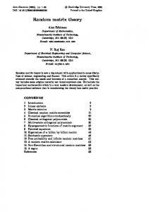
˜ for uniform and nonFigure 2. Fraction of non-zero entries in A uniform sampling. Observe that for all values of p, q = p for uniform sampling and q ≤ p for non-uniform sampling.

To apply Lloyd’s heuristic for k-means clustering we use Matlab’s kmeans function which, by default, uses kmeans++ algorithm (Arthur & Vassilvitskii, 2007) for cluster center initialization. We repeat this clustering 30 times, each time initializing cluster center using k-means++ and selecting the final clustering as the one with lowest k-means objective. We demonstrate the effect of random sparsification obtained by uniform and non-uniform sampling on k-means clustering by reporting the following quantities, (a) 2 > 2 the ratio h1 (q) = kA − Xq X> q AkF /kA − XX AkF , (b) cluster quality h2 (q), measured by normalized mutual information (with respect to ground truth cluster labels of ˜ whose q fracation of enA) of a sparse data matrix A tries are non-zero, and (c) normalized objective function 2 2 h3 (q) = kA − Xq X> q AkF /kAkF , as we vary q. In the above description, Xq is the cluster indicator matrix ob˜ whose q tained by running k-means on sparse data matrix A fraction of entries are non-zero and X is the cluster indicator matrix obtained by running k-means on A. For uniform sampling, p simply indicates that p fraction 4

It has been shown (Cohen et al., 2015) that such dimensionality reduction introduces (1 + ) relative error to optimal k-means objective. We chose projected dimension to be 1000 since increasing it further did not increase normalized mutual information significantly.

where, f > 1, is for pto be chosen later. Therefore, √ τij < p×f , pij = τij × p × f = p×(|A(i, j)|/b)× f . The basic idea is still same as before, i.e., when τij is small, instead of setting pij ∝ (A(i, j))2 , we set pij ∝ |A(i, j)|. Now consider the case when τij < p × f ,P for all i, j. √ The expected number of non-zero entries is i,j p × f × √ (|A(i, j)|/b) = pnd× f ×Avg(|A(i, j)|/b). Therefore, if we choose5 f = 1/(Avg(|A(i, j)|/b))2 , expected number ˜ is pnd. In general, when the condiof non-zero entries in A tion τij < p × f does not hold for all i, j, the expected fraction will be even less since pij < p, for τij ≥ p × f . In our experimental setting, we set f = 1/(Avg(|A(i, j)|/b))2 . This ensures for any p, non-uniform sampling results in at ˜ In our experiments, most p fraction of non-zero entries in A. we vary p from 0.01 to 1.0 in steps of 0.01 and for each ˜ obtained value of p, the number of of non-zero entries in A due to non-uniform sampling is denoted by q and is plotted in Figure 2 for all three datasets. Observe that for all values of p, q = p for uniform sampling and q ≤ p for non-uniform sampling. Next, in Figure 3 we show how random sparsification affects k-means clustering quality with increasing q. As can be seen from Figure 3, with increasing q, h1 (q) and h3 (q) decrease, while h2 (q) increases as one would expect. In fact, h1 (q) decreases quickly towards its optimal value 1 and corresponding h2 (q) value quickly increases towards optimal k-means normalized mutual information of A. The normalized k-means objective h3 (q) also shows steady decrease with increasing q. As can be seen from Figure 3, for all three datasets, non-uniform sampling yields better k-means clustering performance compared to uniform sampling. This makes perfect sense since non-uniform sampling, unlike uniform sampling, enforces sparsity by retaining entries with probability that depends on their magnitude. In fact, for TDT2 and RCV1 datasets, non-uniform sampling results in significant improvement in k-means clustering performance compared to uniform sampling. 5

Avg(|A(i, j)|) represents average over all entries |A(i, j)|.

K-means clustering using random matrix sparsification USPS

2

TDT2

1.2 uniform non-uniform

1.8

RCV1

1.2 uniform non-uniform

1.15

uniform non-uniform

1.15

1.4

1.05

1.2

1

h1(q)

1.1

h1(q)

h1(q)

1.1 1.6

1.05 1

1

0.95

0.95 0

0.1

0.2

0.3

0.4

0.5

0.6

0.7

0.8

0.9

1

0.9 0

0.1

0.2

0.3

0.4

q

0.5

0.6

0.7

0.8

0.9

1

0

0.1

0.2

0.3

0.4

q

0.8

0.6

0.7

0.8

0.9

1

0.6

0.7

0.8

0.9

1

0.6

0.7

0.8

0.9

1

q

0.5

0.6 0.5

0.4

0.6

0.5

0.3

h2(q)

h2(q)

h2(q)

0.4 0.4

0.3

0.2 0.2 0.2

0.1

0

0.1

0 0

0.1

0.2

0.3

0.4

0.5

0.6

0.7

0.8

0.9

1

0 0

0.1

0.2

0.3

0.4

q

0.6

0.7

0.8

0.9

1

0

0.1

0.2

0.3

0.4

q

0.45

0.98

0.96

h3(q)

h3(q)

0.9

0.35

0.5

q

0.95

0.4

h3(q)

0.5

0.85

0.3

0.94

0.92 0.8

0.25

0.2

0.9

0.75 0

0.1

0.2

0.3

0.4

0.5

0.6

0.7

0.8

0.9

1

0.88 0

0.1

0.2

0.3

0.4

q

0.5

0.6

0.7

0.8

0.9

1

q

0

0.1

0.2

0.3

0.4

0.5

q

Figure 3. Effect of random sparsification obtained by uniform and non-uniform sampling on k-means clustering. In all the subplots, red curve indicates uniform sampling and blue curve indicated non-uniform sampling. The black line in the second row indicates normalized mutual information obtained by performing k-means clustering on original data matrix A.

6. Conclusion In this paper we proposed a simple algorithm for k-means clustering using random matrix sparsification and presented its analysis. We proved that under mild condition, for any  ∈ (0, 1), a dense data matrix A ∈ Rn×d can be randomly ˜ ∈ Rn×d containing sparsified to yield a data matrix A 4 9 O(nk/ + d log n) non-zero entries in expectation, such ˜ that an (1 + )-approximate k-mean clustering solution of A results in (1 + O())-approximate clustering solution of A with high probability. Empirical results on three real world datasets demonstrated that k-means clustering solution of ˜ was indeed very close to k-means clustering solution A of A. Moreover, sparsification obtained by non-uniform sampling resulted in better cluster quality compared to uniform sampling. Empirical results also seem to suggest that the O(1/9 ) dependence on the number of non-zero entries ˜ is possibly a bit loose. We conclude this paper with in A two possible open questions: (a) Is it possible to analytically provide a better estimate (by improving dependence on 1/) of the number of non-zero entries in the sparse ma˜ that ensures (1 + ) approximation guarantee? and, trix A (b) Using different proof technique, is it possible to show ˜ will result in that γ-approximate clustering solution of A γ(1 + )-approximate solution of A as shown in Corollary 1, even for γ > 2? In other words, is the restriction on γ

in Corollary 1 a limitation of the proof technique or does it indicate computational hardness of the problem?

References LIBSVM Data: M-ulti-class (classification). URL https://www.csie.ntu.edu.tw/˜cjlin/ libsvmtools/datasets/multiclass.html. Last accessed: 02-05-2018. Achlioptas, D. and Mcsherry, F. Fast computation of low-rank matrix approximations. J. ACM, 54(2), April 2007. ISSN 0004-5411. doi: 10.1145/1219092. 1219097. URL http://doi.acm.org/10.1145/ 1219092.1219097. Arthur, D. and Vassilvitskii, S. K-means++: The advantages of careful seeding. In 18th Annual ACM-SIAM Symposium on Discrete Algorithms, 2007. Bottesch, T., Buhler, T., and Kachele, M. Speeding up kmeans by approximating euclidean distances via block vectors. In 33rd International Conference on Machine Learning, 2016. Boutsidis, C., Zouzias, A., and Drineas, P. Random projections for k-means clustering. In 24th Annual Conference on Neural Information Processing Systems, 2010.

K-means clustering using random matrix sparsification

Boutsidis, C., Zouzias, A., Mahoney, M. W., and Drineas, P. Randomized dimensionality reduction for k-means clustering. IEEE Transactions on Information Theory, 61(2):1045–1062, 2015. Cieri, C., Graff, D., Liberman, M., Martey, N., and Strassel, S. The TDT-2 text and speech corpus. In DARPA Broadcast News Workshop, 1999. Cohen, M. B., Elder, S., Musco, C., Musco, C., and Persu, M. Dimensionality reduction for k-means clustering and low rank approximation. In 47th Annual Symposium on Theory of Computing, 2015. Dasgupta, S. The Hardness of K-means Clustering. Technical report (University of California, San Diego. Department of Computer Science and Engineering). Department of Computer Science and Engineering, University of California, San Diego, 2008. URL https://books. google.com/books?id=riJuAQAACAAJ. Ding, Y., Zhao, Y., Shen, X., Musuvathi, M., and Mytkowicz, T. Yinyanh k-means: A drop-in replacement of the classic k-means with consistent speedup. In 32nd International Conference on Machine Learning, 2015. Drake, J. and Hamerly, G. Accelerated k-means with adaptive distance bounds. In 5th NIPS Workshop on Optimization for Machine Learning, 2012. Elkan, C. Using triangle inequality to accelerate k-means. In 20th International Conference on Machine Learning, 2003. Feldman, D. and Langberg, M. A unified framework for approximating and clustering data. In 43rd Annual ACM Symposium on Theory of Computing, 2011. Feldman, D., Schmidt, M., and Sohler, C. Turning big data into tiny data: Constant-size coresets for k-means, pca and projective clustering. In 24th Annual ACM-SIAM Symposium on Discrete Algorithms, 2013. Hamerly, G. Making k-means even faster. In SIAM International Conference on Data Mining, 2010. Hull, J. J. A database for hand written text recognition research. IEEE Transactions on pattern Analysis and machine Intelligence, 16(5):550 – 554, 1994. Lewis, D. D., Yang, Y., Rose, T. G., and Li, F. RCV1: A new benchmark collection for text categorization research. Journal of Machine Learning Research, 5:361 – 397, 2004. Liu, W., Shen, X., and Tsang, I. W. Sparse embedded kmeans clustering. In 31st Annual Conference on Neural Information Processing Systems, 2017.

Lloyd, S. Least square quantization in PCM. IEEE Transactions on Information Theory, 28(2):129 – 137, 1982. Mirsky, L. Symmetric gauge functions and unitarily invariant norms. The Quarterly Journal of Mathematics, 11:50 – 59, 1960. Newling, J. and Fleuret, F. Fast k-means with accurate bounds. In 33rd International Conference on Machine Learning, 2016. Wu, X. Top 10 algorithms in data mining. Knowledge and Information Syaytems, 14(1):1 – 37, 2008.