In the case of standard linear PCA, the algorithm can be formulated as minimization for .... For example, in linear algebra we use it in connection with fields, rings and groups ...... By a quantitative analysis, Meckes (2009) has been shown the.
Kernel Choice for Unsupervised Kernel Methods
A dissertation submitted in partial fulfillment of the requirements for the degree Doctor of Philosophy
by Md. Ashad Alam
in Department of Statistical Science The Institute of Statistical Mathematics The Graduate University of Advanced Studies Tokyo 190-8562, Japan.
September 2014
c Copyright⃝ Md. Ashad Alam, September 2014 All rights reserved.
I
The dissertation of Md. Ashad Alam is approved, and it is acceptable in quality and form for publication on microfilm and electronically.
Prof. Satoshi Kuriki
Dr. Shotaro Akaho
Prof. Daichi Mochihashi
Prof. Kenji Fukumizu Adviser
Prof. Koji Kanefuji Department Head/ Director
September 2014
II
DEDICATION
Our motherland Gˆonˆoprˆojatˆontri Bangladesh (The People’s Republic of Bangladesh)
III
EPIGRAPH
Without Modern Mathematics Statistics, Robust Statistics and Statistical Machine Learning are like Gardening without any Flowers.
IV
Contents 1 Introduction
1
1.1
Designing kernel for unsupervised kernel methods . . . . . . . . . . . . . .
4
1.2
Robustness of unsupervised kernel methods . . . . . . . . . . . . . . . . .
5
1.3
Scope of the research . . . . . . . . . . . . . . . . . . . . . . . . . . . . .
5
1.4
Outline and summary of the contributions . . . . . . . . . . . . . . . . . .
6
2 Preliminary
7
2.1
Inner product space . . . . . . . . . . . . . . . . . . . . . . . . . . . . . .
2.2
Hilbert space . . . . . . . . . . . . . . . . . . . . . . . . . . . . . . . . . 10
2.3
Feature space and its drawback . . . . . . . . . . . . . . . . . . . . . . . . 12
2.4
2.5
2.6
8
2.3.1
Feature space . . . . . . . . . . . . . . . . . . . . . . . . . . . . . 14
2.3.2
Computational problems of feature space . . . . . . . . . . . . . . 14
Kernel and positive definite kernel . . . . . . . . . . . . . . . . . . . . . . 15 2.4.1
Kernel . . . . . . . . . . . . . . . . . . . . . . . . . . . . . . . . . 15
2.4.2
Advantages of kernel . . . . . . . . . . . . . . . . . . . . . . . . . 18
2.4.3
Positive definite kernel (PDK) . . . . . . . . . . . . . . . . . . . . 19
2.4.4
Well-known PDKs and its parameters . . . . . . . . . . . . . . . . 21
2.4.5
Valid PDKs and its matrices . . . . . . . . . . . . . . . . . . . . . 24
2.4.6
Properties of PDKs . . . . . . . . . . . . . . . . . . . . . . . . . . 26
2.4.7
Interplay between PDK, reproducing kernel and Mercer kernel . . . 31
Reproducing kernel Hilbert space (RKHS) . . . . . . . . . . . . . . . . . . 33 2.5.1
Properties of RKHS . . . . . . . . . . . . . . . . . . . . . . . . . 34
2.5.2
Representer theorem . . . . . . . . . . . . . . . . . . . . . . . . . 37
Methods based on RKHS . . . . . . . . . . . . . . . . . . . . . . . . . . . 38 V
2.6.1
Supervised learning . . . . . . . . . . . . . . . . . . . . . . . . . . 39
2.6.2
Unsupervised learning . . . . . . . . . . . . . . . . . . . . . . . . 39
2.6.3
Nonparametric inference . . . . . . . . . . . . . . . . . . . . . . . 39
3 Automatic Way of Finding Hyperparameters in Kernel Principal Component Analysis 3.1
3.2
3.3
3.4 4
40
Motivation . . . . . . . . . . . . . . . . . . . . . . . . . . . . . . . . . . . 40 3.1.1
Kernel principal component analysis (kernel PCA) . . . . . . . . . 42
3.1.2
Choice of kernel . . . . . . . . . . . . . . . . . . . . . . . . . . . 43
Proposed methods . . . . . . . . . . . . . . . . . . . . . . . . . . . . . . 45 3.2.1
Pre-Image of kernel PCA . . . . . . . . . . . . . . . . . . . . . . . 45
3.2.2
Hyperparameters choice . . . . . . . . . . . . . . . . . . . . . . . 47
3.2.3
Computational cost . . . . . . . . . . . . . . . . . . . . . . . . . . 48
Experimental results . . . . . . . . . . . . . . . . . . . . . . . . . . . . . 49 3.3.1
Synthesized data . . . . . . . . . . . . . . . . . . . . . . . . . . . 49
3.3.2
Real world problems . . . . . . . . . . . . . . . . . . . . . . . . . 51
3.3.3
Polynomial kernel . . . . . . . . . . . . . . . . . . . . . . . . . . 52
Discussion . . . . . . . . . . . . . . . . . . . . . . . . . . . . . . . . . . 53
Classical, Robust and Kernel Canonical Correlation Analysis
58
4.1
Motivation . . . . . . . . . . . . . . . . . . . . . . . . . . . . . . . . . . . 58
4.2
Classical and robust canonical correlation analysis . . . . . . . . . . . . . . 59
4.3
Measure of robustness . . . . . . . . . . . . . . . . . . . . . . . . . . . . 61 4.3.1
Qualitative robustness . . . . . . . . . . . . . . . . . . . . . . . . 61
4.3.2
Influence function . . . . . . . . . . . . . . . . . . . . . . . . . . 61
4.3.3
Breakdown point . . . . . . . . . . . . . . . . . . . . . . . . . . . 62
4.4
Kernel canonical correlation analysis . . . . . . . . . . . . . . . . . . . . 62
4.5
Experimental results . . . . . . . . . . . . . . . . . . . . . . . . . . . . . 64 4.5.1
Simulation results . . . . . . . . . . . . . . . . . . . . . . . . . . 65
4.5.2
Sensitivity analysis . . . . . . . . . . . . . . . . . . . . . . . . . . 70
4.5.3
Breakdown analysis . . . . . . . . . . . . . . . . . . . . . . . . . 70
VI
5 Higher-order Regularized Kernel Canonical Correlation Analysis
74
5.1
Motivation . . . . . . . . . . . . . . . . . . . . . . . . . . . . . . . . . . . 74
5.2
Cross-validation for the standard kernel canonical correlation analysis . . . 75
5.3
Distribution of a low dimensional projection . . . . . . . . . . . . . . . . 77
5.4
Higher-order regularized kernel CCA (hrKCCA) . . . . . . . . . . . . . . 80
5.5
5.4.1
Method . . . . . . . . . . . . . . . . . . . . . . . . . . . . . . . . 80
5.4.2
Kernel choice for hrKCCA . . . . . . . . . . . . . . . . . . . . . . 82
5.4.3
Computational issues . . . . . . . . . . . . . . . . . . . . . . . . . 83
Experiments . . . . . . . . . . . . . . . . . . . . . . . . . . . . . . . . . . 84 5.5.1
Synthesized examples . . . . . . . . . . . . . . . . . . . . . . . . 84
5.5.2
Real world datasets . . . . . . . . . . . . . . . . . . . . . . . . . . 87
6 Conclusion and Future Research
105
6.1
Conclusion . . . . . . . . . . . . . . . . . . . . . . . . . . . . . . . . . . 105
6.2
Future research . . . . . . . . . . . . . . . . . . . . . . . . . . . . . . . . 107
VII
List of Tables 2.1
Examples of well-known positive definite kernels and its parameters. . . . . 23
3.1
Computational cost (in second) of the proposed method for synthesized data-2 with different data sizes (n) and the numbers of components (ℓ) . . . 48
3.2
The configuration of datasets for hyperparmeters choice in kernel principal component analysis (kernel PCA). . . . . . . . . . . . . . . . . . . . . . . 50
3.3
Five real-world data sets: leave-one-out cross validation (LOOCV) reconstruction errors and LOOCV classification errors for inverse bandwidths (s) and the number of components (ℓ). The minimum values are written in bold fonts, and the classification errors with the hyperparameters chosen by the proposed method are underlined. . . . . . . . . . . . . . . . . . . . 55
3.4
USPSG-500: LOOCV reconstruction errors and LOOCV classification errors (bold numbers indicate the minimum value). . . . . . . . . . . . . . . 56
3.5
LOOCV reconstruction errors for food data. . . . . . . . . . . . . . . . . . 56
3.6
Polynomial kernel for wine data: LOOCV reconstruction errors and the LOOCV classification errors (bold numbers indicate the minimum value). . 57
4.1
Bias and mean square error of simulated data (bold numbers indicate the minimum value). . . . . . . . . . . . . . . . . . . . . . . . . . . . . . . . 66
4.2
The value of qualitative robustness index. . . . . . . . . . . . . . . . . . . 66
5.1
Time complexity (in second) for example 3: the proposed kernel CCA with three numbers of iterations (I) and the standard kernel CCA (KCCA). The Gaussian kernel is used for the both methods, and n is the sample size. . . . 84
VIII
5.2
The configuration of datasets along with purposes (estimate of dependence feature (EDF), measure of association (MA) and estimate of low dimensional space (ELDS)) of all experimental datasets. . . . . . . . . . . . . . . 85
5.3
Cross-validation errors of the three examples (E1 − E3 ) using different inverse bandwidths s and regularization coefficients λ for the proposed method and standard kernel CCA (KCCA). . . . . . . . . . . . . . . . . . 87
5.4
Cross-validation errors for nutrimouse dataset. . . . . . . . . . . . . . . . . 88
5.5
Classification errors (%) for wine, BUPA liver disorders and diabetes. One or two dimensional features are used with the proposed method (hrKCCA+kNN and hrKCCA+SVM) and the kernel CCA. . . . . . . . . . . . . . . . . . . 91
5.6
Classification errors (%) using one dimensional estimated subspace of DBWorld subject and bodies datasets by the proposed method (hrKCCA+kNN and hrKCCA+SVML ) other exiting methods. . . . . . . . . . . . . . . . . 93
5.7
Recognition rate (%) for KTH dataset (all scenarios) by the proposed method (hrKCCA+kNN and hrKCCA+SVML ) and other methods. . . . . . . . . . 94
5.8
Recognition rate (%) for UMD dataset by the proposed method (hrKCCA+kNN and hrKCCA+SVML ) and some of the best stat-of-the-art methods of this dataset. . . . . . . . . . . . . . . . . . . . . . . . . . . . . . . . . . . . . 95
IX
List of Figures 2.1
Background of the kernel in the 20th century. . . . . . . . . . . . . . . . . 16
3.1
Individual reproducing kernel Hilbert space for each kernel of the kernel principal component analysis (KPCA). . . . . . . . . . . . . . . . . . . . . 44
3.2
Scatter plots of the first two kernel principal components for wine data: Gaussian RBF kernel is used in the top panel (a) s = 0.05 (b) s = 0.75 (c) s = 1 (d) s = 10, and polynomial kernel in the bottom (e) c = 0.001, d = 2 (f) c = 10, d = 2 (g) c = 1, d = 3 (h) c = 1, d = 4. . . . . . . . . . . . . . . 45
3.3
Architecture of kernel choice in kernel PCA. . . . . . . . . . . . . . . . . . 48
3.4
Algorithm of kernel choice in kernel PCA with Gaussian RBF kernel. . . . 49
3.5
Kernel PCA for synthesized data-1 (top) and synthesized data-2 (bottom). (a) Scatter plot for the two variables of a sample. (b) Box plots of the leaveone-out cross validation (LOOCV) reconstruction errors for 100 samples. (c, d) scatter plots of the first two kernel principal components using (c) the best inverse kernel widths (s = 5, 10) and (d) larger bandwidths s = 50, 200. 51
3.6
Visualization of the first two kernel principal components of food data (a) s = 0.001, (b) s = 0.5 and (c) s = 200 . . . . . . . . . . . . . . . . . . . . 53
4.1
The system of CCA. . . . . . . . . . . . . . . . . . . . . . . . . . . . . . 60
4.2
The system of kernel CCA. . . . . . . . . . . . . . . . . . . . . . . . . . . 63
4.3
Box plots of canonical correlation coefficient of five estimators using population canonical correlation, PCC = 0.79 and PCC = 0.63. . . . . . . . . . 67
4.4
Scatter plots of (X1 , Y1 ) (top left) and first canonical variates . . . . . . . . 68
4.5
Scatter plots of (X2 , Y2 ) (top left) and 2nd canonical variates . . . . . . . . 69
X
4.6
Box plots of sensitivity value over 200 samples a) multivariate normal data and b) transform multivariate normal data. . . . . . . . . . . . . . . . . . . 71
4.7
Breakdown plots for first canonical correlation coefficient. . . . . . . . . . 73
5.1
Standard kernel CCA: the scatter plots of the 1st canonical variates for the nutrimouse dataset (liver cells and hepatic fatty acids) using the Gaussian RBF kernel with eight inverse bandwidths s and fixed regularization coefficient κ = 10−4 . The 10-fold cross-validation errors are also embedded. . . 78
5.2
Algorithm of the higher-order regularized kernel CCA. . . . . . . . . . . . 83
5.3
Scatter plots of 1st kernel canonical variates for the examples (E1 −E3 ). The first column for the standard kernel CCA. The final three columns for the hrKCCA, using different trade-off c for the regularization parameters: ν = cλ. The inverse bandwidth s and the 4th moment regularization coefficient λ are chosen by the CV. . . . . . . . . . . . . . . . . . . . . . . . . . . . . 96
5.4
Box plots and line plots (inset) using mean values of cross-validation errors of 100 samples for example 3 (bandwidths, s1 = 225, s2 = 250, s3 = 275, s4 = 300, s5 = 325, s6 = 350, s7 = 375, s8 = 400). . . . . . . . . . . . . 97
5.5
Scatter plots of the 1st kernel canonical variates given by the proposed method for the nutrimouse dataset (liver cells and hepatic fatty acids) using the Gaussian RBF kernel with eight inverse bandwidths s and fixed regularization coefficient λ = 0.75. The 10-fold cross-validation error is also embedded (see also Table 5.4). . . . . . . . . . . . . . . . . . . . . . . . . 98
5.6
Scatter plots of the first canonical variates of real datasets (Email (D2 ), Psychological (D3 ) and Carbig (D4 )) using the parameters chosen by CV for the kernel CCA (a) and the proposed method (b). . . . . . . . . . . . . 99
5.7
Scatter plots of the first canonical variates (a(i)) -(d(i)) and the first two canonical variates of the exploratory variables (a(ii) -d(ii)) for the wine dataset. The proposed method (s = 0.05, λ = 0.1) in (a) and kennel CCA using three heuristic bandwidths (s1 = 0.02, s2 = 0.073, s3 = 0.05) in (b d) are shown. . . . . . . . . . . . . . . . . . . . . . . . . . . . . . . . . . 100
XI
5.8
Scatter plots of the first canonical variates (upper row) and one dimensional index plots (lower row) given by the proposed method for DBWorld subject, bodies, BUPA liver disorders, and diabetes. . . . . . . . . . . . . . . . . . 101
5.9
Scatter plots of the first canonical variates (upper row) and the first two canonical variates of X (lower row) using KTH dataset (outdoor scenario only) for the kernel CCA. . . . . . . . . . . . . . . . . . . . . . . . . . . . 102
5.10 Scatter plots of the first canonical variates (upper row) and first two canonical variates of X (lower row) using KTH dataset (outdoor scenario only) for the proposed hrKCCA. . . . . . . . . . . . . . . . . . . . . . . . . . . 103 5.11 Scatter plots of the first canonical variates (upper row), first two canonical variates of X (middle row) and confusion matrices (lower row) using KTH dataset for all scenarios (boxing (B), hand clapping (HC), hand waving (HW), jogging (J), running (R), and walking (W)) for the for the proposed hrKCCA. . . . . . . . . . . . . . . . . . . . . . . . . . . . . . . . . . . . 104
XII
ACKNOWLEDGMENTS
First and foremost, I would like to pay my thanks to my adviser, Professor Kenji Fukumizu, The Institute of Statistical Mathematics (ISM) and The Graduate University of Advanced Studies (SOKENDAI). I owe a great deal of gratitude to him for his guidance, financial support and help throughout the exciting journey full of learning and growth at my doctoral courses and research in Japan. I would like to extend my thanks to the faculty members, especially Professor Shinto Eguchi, Professor Satoshi Ito, Dr. Yoichi Nishiyama who taught me during the doctoral courses. It’s my pleasure to thank to Dr. Osamu Komori. He served me as a family member in the last five years in Japan. I will keep them my mind always who had assisted me cordially in getting relevant literatures and other necessary advice. I acknowledge to the staffs of ISM and research Cooperation Unit (Kenkyo) for their cordial help and co-operation during my research work. I am very grateful to Dr. Takao Kumazawa for his excellent guidance and sightseeing in Tokyo during first two years. I would like to express my heartfelt gratitude to all Fukumizu’s lab members and friends who have supported me through the years and have made my time at ISM so enjoyable. In particular, I would like to thank Dr. Akifumi Notsu, Yuta Tanoue, Hisaki Ikebata and Katsuhiro Omae with whom I share many unforgettable memories. One thing I must confess, without the encouragement and care all though my life, of my parents Md. Shamsul Alam Akando and Mst. Helena Alam would be quite impossible to continue the doctoral course and research. I would like to thank all of my family members and relatives. My special thanks go my M.Sc. adviser, Professor Mohammed Nasser University of Rajshahi, who encourages a lot to begin my research. At last, my deepest gratitude and love, of course, belongs to my wife, Mst. Shajia Afrin, my daughter, Asfia Alsaba and my son, Saffat Ashad for their unconditional love and help. They are one of my main sources of inspiration.
XIII
ABSTRACT OF THE DISSERTATION by Md. Ashad Alam in Department of Statistical Science The Institute of Statistical Mathematics The Graduate University of Advanced Studies Tokyo 190-8562, Japan.
In kernel methods, choosing a suitable kernel is indispensable for favorable results. While cross-validation is a useful method of the kernel and parameter choice for supervised learning such as the support vector machines, there are no well-founded methods, have been established in general for unsupervised learning. We focus on kernel principal component analysis (kernel PCA) and kernel canonical correlation analysis (kernel CCA), which are the nonlinear extension of principal component analysis (PCA) and canonical correlation analysis (CCA), respectively. Both of these methods have been used effectively for extracting nonlinear features and reducing dimensionality. As a kernel method, kernel PCA and kernel CCA also suffer from the problem of kernel choice. Although cross-validation is a popular method of choosing hyperparameters, it is not applicable straightforwardly to choose a kernel and the number of components in kernel PCA and kernel CCA. It is important, thus, to develop a well-founded method for choosing hyperparameters of the unsupervised methods. In kernel PCA, it is not possible to use cross-validation for choosing hyperparameters because of the incomparable norms given by different kernels. The first goal of the dissertation is to propose a method for choosing hyperparameters in kernel PCA (the kernel and the number of components) based on cross-validation for the comparable reconstruction errors of pre-images in the original space. The experimental results of synthesized and real-world datasets demonstrate that the proposed method successfully selects an appropriate kernel and the number of components in kernel PCA in terms of visualization and classification errors on the principal components. The results imply that the proposed method enables the automatic design of hyperparameters in kernel PCA. XIV
In recent years, the influence function of kernel PCA and a robust kernel PCA has been theoretically derived. One observation of their analysis is that kernel PCA with a bounded kernel such as Gaussian is robust in that sense the influence function does not diverged, while for kernel PCA with unbounded kernels for example polynomial the influence function goes to infinity. This can be understood by the boundedness of the transformed data onto the feature space by a bounded kernel. While this is not a result of kernel CCA but for kernel PCA, it is reasonable to expect that kernel CCA with a bounded kernel is also robust. This consideration motivates us to do some empirical studies on the robustness of kernel CCA. It is essential to know how kernel CCA is effected by outliers and to develop measures of accuracy. Therefore, we do intend to study a number of conventional robust estimates and kernel CCA with different functions but fixed parameter of kernel. The second goal of the dissertation is to discuss five canonical correlation coefficients and investigate their performances (robustness) by influence function, sensitivity curve, qualitative robustness index and breakdown point using different type of simulated datasets. The final goal of the dissertation is to extract the limitations of cross-validation for the kernel CCA, and to propose a new regularization approach to overcome the limitations of kernel CCA. As we demonstrate for Gaussian kernels, the cross-validation errors for kernel CCA tend to decrease as the bandwidth parameter of the kernel decreases, which provides inappropriate features with all the data concentrated in a few points. This is caused by the ill-posedness of the kernel CCA with the cross-validation. To solve this problem, we propose to use constraints on the 4th order moments of canonical variables in addition to the variances. Experiments on synthesized and real world datasets including human action recognition for a robot demonstrate that the proposed higher-order regularized kernel CCA can be applied effectively with the cross-validation to find appropriate kernel and regularization parameters.
XV
Chapter 1 Introduction Methods using positive definite kernel (PDK), kernel methods play an increasingly prominent role to solve various problems in statistical machining learning such as, web design, pattern recognition, human action recognition for a robot, computational protein function perdition, remote sensing data analysis and in many other research fields. Due to the kernel trick and reproducing property, we can use linear techniques in feature spaces without knowing explicit forms of either the feature map or feature spaces. It offers versatile tools to process, analyze, and compare many types of data and offers state-of-the-art performance. Nowadays, PDK has become a popular tool for the most branches of statistical machine learning e.g., supervised learning, unsupervised learning, reinforcement learning, non-parametric inference and so on. Many methods have been proposed to kernel methods, which include support vector machine (SVM, Boser et al., 1992), kernel ridge regression (KRR, Saunders et al., 1998), kernel principal component analysis (kernel PCA, Sch¨olkopf et al., 1998), kernel canonical correlation analysis (kernel CCA, Akaho, 2001, Bach and Jordan, 2002), Bayesian inference with positive definite kernels (kernel Bayes’ rule, Fukumizu et al., 2013), gradient-based kernel dimension reduction for regression (gKDR, Fukumizu and Leng, 2014), kernel two-sample test (Gretton, 2012) and so on. During the last decade, unsupervised learning has become an important application area of the kernel methods. There are two most powerful tools of unsupervised kernel methods, namely kernel principal component analysis (kernel PCA) and kernel canonical correlation analysis (kernel CCA) (Sch¨olkopf et al., 1998, Akaho, 2001). Using these two methods, we are able to extract effective nonlinear features by high dimensional embedding of data
Introduction based on the reproducing kernel Hilbert space (RKHS). They have also closed connection with many unsupervised dimensional reductions and manifold learning techniques (Izenman, 2008, Chapter 16). Kernel PCA and kernel CCA have been applied in different areas of statistical machine learning such as reduction of dimensionality, image processing, feature extraction, de-noising, statistical shape analysis, novelty detection, pre-processing of regression and classification (Mika et al., 1999, Kwok and Tsang, 2003, Arias et al., 2007, Zheng et al., 2010, Hardoon et al., 2004, Huang et al., 2009a, Alzate and Suykens, 2008). In all of the above areas, kernel PCA and kernel CCA have been used with an arbitrary choice of the kernel and the number of features. The results are in fact very sensitive to both the choice of the kernel and the number of features of RKHS. As a kernel method, kernel PCA and kernel CCA also suffer from the problem of kernel choice. To the best of our knowledge, however, a well-founded technique for choosing the parameters has not yet been established. The cross-validation (CV) approach is popularly used for choosing parameters of kernel methods, such as the bandwidth parameter in Gaussian kernel, especially in supervised learning. For SVM, the cross-validation is one of the most popular and useful ways of choosing the kernel and parameters (Arlot, 2010, Woen and Perry, 2009, Stone, 1974). In the case of standard linear PCA, the algorithm can be formulated as minimization for self-regression with reduced rank, and cross-validation approaches have been proposed for choosing the number of components (Krzanowski, 1987, Wold, 1978). The k-fold CV has been used for classical CCA (Liang, 1995). Note that it is not possible to apply the leave-one-out CV (LOOCV) with canonical correlation value, since the correlation is not computable with one data. While the CV with the canonical correlation value has been used for choosing the bandwidth in kernel CCA (Suetani et al., 2006), where very dense data from a chaotic dynamics are discussed, it is not easy in general to obtain reliable canonical correlation values by the k-fold CV for small data points. The result of kernel PCA obviously depends on the choice of the kernel. It is often the case that the kernel has some parameters like the popular examples shown in Table 2.1. In such a case, these parameters may have a strong influence on the results. To depict the influence, using wine dataset we show the plots of the first two kernel principal components with different values of inverse-bandwidth parameters in the Gaussian RBF kernel, and
2
Introduction degree and constant in the polynomial kernel (see Section 3.3 and Figure 3.2). From the figures, we see that in both the kernels the results of kernel PCA depend strongly on the parameters, and an appropriate choice is indispensable for the method to give reasonable low-dimensional representation of data. In kernel CCA with Gaussian RBF kernel, we need to select a proper inverse bandwidth and a regularization parameter. It is also well known each hyperparameter has the influence on the result of kernel CCA. A guideline to select the regularization parameter has been proposed by Hardoon et al. (2004) and a heuristic technique has been also used for choosing the bandwidth (Hardoon and Shawe-Taylor, 2009). It is known that CCA and kernel CCA can be regarded as an alternating regression problem (Breiman and Friedman, 1985, Shawe-Taylor and Cristianini, 2004). CV using correlations or prediction error depends on the data concentration. When the data are concentrated in only a few extreme points with perfect or nearly perfect correlations, on the one hand, the CV error will be very small which satisfies the objective of kernel CCA (maximum correlation of canonical variate) but on the other hand, the canonical variates do not follow any well-posed distribution. In classification problems, we can use CV based on classification rates, but the smallest classification error does not correspond to the high correlated features of kernel CCA, in general. For kernel CCA, however, the cross-validation approach based on the prediction error does not necessarily choose a good parameter in general. We demonstrate this problem using an example of the nutrimouse dataset for the Gaussian RBF kernel (see the Chapter 5). In Figures 5.1 we show eight scatter plots of the first canonical variates using eight inverse bandwidths together with the cross-validation errors. As we see, the larger value of inverse bandwidth provides smaller error (≈ 0), but the solution are ill-posed: high correlation is achieved by the features with most data concentrating on a few points. This example illustrates that a straightforward application of cross-validation for choosing a kernel is not appropriate. It is expected that the variance constraints on the kernel CCA do not regulate sufficient for a large variety of nonlinearity given by different kernels. Although cross-validation is a popular method for choosing hyperparameters, it is not applicable straightforwardly to choose a kernel of kernel PCA and kernel CCA. It is important, thus, to develop a well-founded method of designing a kernel of unsupervised
3
Introduction kernel methods. The main goal of the dissertation is to design a kernel and robustness for unsupervised kernel methods.
1.1 Designing kernel for unsupervised kernel methods Selection of hyperparameters (kernel and the number of features) of kernel PCA is not a straightforward task because each kernel provides an individual norm in corresponding feature space. So, we are not able to choose them based on a performance with the norms of the feature spaces. In Chapter 3, we propose a method for choosing an optimum kernel and the number of features through the LOOCV based on pre-image performance, which is an approximate inverse image of a point in the feature space. To this ends, we extract the pre-image of a test point projected onto the subspace in RKHS using a pre-image method of each feature space. We then evaluate the reconstruction error based on this pre-image. As in the leave-one-out cross-validation, each data set is regarded as a test point and the average error is computed. The kernel and the number of features corresponding to the minimum error is chosen as the optimum ones. As the kernel PCA, selection of the kernel and the number of features for kernel CCA is also a challenging problem. We are not able to extract the kernel CCA fruitfully by LOOCV. Canonical correlation analysis is the generalization of regression analysis with multiple response variables. So, it is possible to use mean square error like as regression analysis to apply LOOCV. By this result, we have observed that for small bandwidth of Gaussian RBF kernel, the most of data points are accumulated but for a few extreme points. In this situations, the CV error is very small. Moreover, the CV values highly to depends on bandwidth in finite samples. Kernel CCA is given by the second order statistics (e.g., variance) of the canonical variates; this would suffice for a complete statistical description of a Gaussian distribution, but not in general. With the rich function classes given by positive definite kernels, we need much stronger constraint to regulate the canonical variate sufficiently to make the cross-validation applicable. The kernel CCA subject to the higher-order constraints is proposed to select the tuning parameters using the cross-validation technique. We demonstrate the effectiveness of the proposed higher-order regularized kernel CCA, combined with the
4
Introduction cross-validation, in measuring the relationship and extracting effective features for classification using various synthesized and real world problems (see Chapter 5).
1.2 Robustness of unsupervised kernel methods The influence function (IF) of kernel PCA has been theoretically well-known. Kernel PCA with a bounded kernel such as Gaussian is robust in the sense that the influence function does not diverge, while it is not robust with unbounded kernels for example polynomial (IF goes to infinity). This can be understood by the boundedness of the transformed data onto the feature space by a bounded kernel (Huang et al., 2009b, Suykens et al., 2010). While this is not a result of kernel CCA, it is reasonable to expect that kernel CCA with a bounded kernel is also robust. This consideration motivates us to do some empirical studies on the robustness of kernel CCA. It is essential to know how kernel CCA is affected by outliers and to develop measures of accuracy. Therefore, we intend to study a number of conventional robust estimates and kernel CCA with different functions, but fixed bandwidth of Gaussian RBF kernel and Laplacian kernel (see Chapter 4).
1.3 Scope of the research Kernel PCA and kernel CCA are most useful and fundamental unsupervised statistical pattern recognition techniques as well as preprocessing techniques for supervised learning: regression analysis and classification analysis to predict from massive amounts of data. Both of these techniques are also used in unsupervised learning to extract significant and anomaly structure of high dimensional datasets. Kernel CCA is also used as a constrast function of independent component analysis, an important method of unsupervised learning. An additional important application area of kernel CCA is stochastic processes to learn the dynamic nature of the processes. The proposed two methods provide a way of automatic findings the hyperparemtes of the kernel PCA and kernel CCA. It is expected that our research would be a great impact on the area of statistical machine learning.
5
Introduction
1.4 Outline and summary of the contributions Chapter 1: The motivation of designing the kernel and robustness for unsupervised kernel methods are presented in the first chapter. Chapter 2: A review of important and useful results of functional analysis and PDK is given in this chapter. Chapter 3: This chapter discusses the limitations of kernel PCA and provides a new method for choosing hyperparameters in kernel PCA (kernel and the number of components) based on CV for the comparable reconstruction errors of pre-images in the original space. The proposed method has been applied to synthesized and a number of real world datasets. Chapter 4: This chapter treats the performances of five canonical correlation coefficients in the different types of distribution using influence function, sensitivity curve, qualitative robust index and breakdown point. Chapter 5: This chapter discusses the CV for kernel CCA with its limitations, and provides a new 4th order moment regularization approach for kernel CCA. The proposed method demonstrates for synthesized and real world problems, including human action recognition for a robot. Chapter 6: A conclusion and further aspects of research are discussed in the final chapter.
6
Chapter 2 Preliminary of Functional Analysis and Kernel Functional analysis is an abstract branch of mathematics where the vector spaces are in general infinite dimensional and not all operators on them can be represented by matrices unlike the linear algebra. An abstract approach starts with a set of elements satisfying certain axioms. For example, in linear algebra we use it in connection with fields, rings and groups, but in functional analysis it in connection with abstract spaces (inner product space, Hilbert spaces, Banach spaces etc.,). An abstract space is a set (unspecified) of elements satisfying certain axioms. The different sets of axioms provide different abstract spaces. Functional analysis has a history of more than one century and nowadays its results have been used in a number of areas: mathematics, statistics, robust statistics and statistical machine learning. Some basic definitions and results are summarized in this chapter, which are frequently used to reproducing kernel Hilbert space (RKHS) and its methods. The fundamental references of this chapter are: Hille (1972), Reed and Simon (1980), Kreyszig (1989), Cucker and Smale (2002), Sch¨olkopf and Smola (2002), Berlinet and ThomasAgnan (2004), Shawe-Taylor and Cristianini (2004), Bishop (2006), Steinwart and Christmann (2008), Hofmann et al. (2008), G¨artner (2008), Fukumizu et al. (2009), King (2009), Fasshauer (2011), Steinwart and Scovel (2012) and Fukumizu et al. (2013).
Functional Analysis and Kernel
2.1
Inner product space
In calculus, the notions of convergence and continuity can be formulated in terms of distance between two numbers or between two vectors, where the objects are very simple (R or Rn ). In functional analysis, we consider more general spaces, which contain more complicated objects than numbers and vectors e.g., functions and so on. To find a distance between two complicated objects, we need a new notion of distance that lead a new notion of convergence and continuity. These again lead to new arguments surprisingly similar to those we have already seen in calculus. Now the question, is it possible to develop a general theory of distance where we can prove the results (we need once and for all)? We have a positive answer and the theory is called the theory of metric spaces. By inducing general conditions on the distance function, we are able to develop a general notion of distance, which can be applicabled even on complicated objects. Using metric space theory, we can formulate and prove results about convergence and continuity once and for all. Metric space is a set with a metric on it. We can generalize it by a notion of nearness (open set is sufficient). Simply imagine small open balls around a point to measure nearness without mentioning distances, which leads to the idea of a topological space. The fundamental notion of topological space is based on the collection of all open sets (complement is closed set) instead of metric. The field of topology is an abstract study that evolved as an independent discipline in response to certain problems of classical analysis and geometry. It provides a unifying theory that can be used in many diverse branches of mathematics. The metric and topology are defined on an abstract set, which may or may not be a vector space. To make a relation between algebraic and geometric properties of an abstract set, we need to define a metric in the special form, say norm. A norm is nothing but a metric on the vector space, which is combined the algebraic structure and metric concepts. It can be given more useful and important metric spaces (Kreyszig, 1989). In a normed space we can do vector addition and scalar multiplication of a vector just like the elementary vector algebra, but still we cannot do two useful operations: vector dot product and orthogonality of two vectors. It is possible to fill this gap using the inner product. A vector space together with an inner product is called an inner product space. Definition 2.1.1 (Inner product space) Let V is a vector space (real or complex). The 8
Functional Analysis and Kernel inner product of the V is a continues mapping ⟨, ⟩ : V × V → F, that has the following four properties, where F is a scaler field of V: CI1 (Positive definite) ⟨x, x⟩ ≥ 0,
⟨x, x⟩ = 0 ⇔ x = 0.
CI2 (Anti-symmetric (Hermitian)) ⟨x, y⟩ = ⟨y, x⟩,
∀ x, y ∈ V.
For a real vector space (Symmetric). ⟨x, y⟩ = ⟨y, x⟩,
∀ x, y ∈ V.
CI3 (Homogeneity) ⟨ax, y⟩ = a⟨x, y⟩,
∀a ∈ F.
CI4 (Cumulative (addition)) ⟨x + y, z⟩ = ⟨x, z⟩ + ⟨y, z⟩,
∀x, y, z ∈ V.
The pair (V, ⟨, ⟩) is called inner product space. A metric is a measure of how different the elements of a set are. A norm is a measure of how large the element is. An inner product is a measure of what degree the elements are linearly independent. A useful property of inner products is the Cauchy-Schwarz inequality, 1
1
⟨x, y⟩ ≤ ⟨x, x⟩ 2 ⟨y, y⟩ 2 .
(2.1)
This relationship is also sometimes called the Cauchy-Bunyakovskii-Schwarz inequality. 9
Functional Analysis and Kernel
2.2 Hilbert space Hilbert spaces are possibly-infinite-dimensional analogues of the finite-dimensional Euclidean spaces familiar to us. In particular, Hilbert spaces have inner products, so notions of perpendicularity (or orthogonality) and orthogonal projection are available. Reasonably enough, in the infinite-dimensional case we must be careful not to extrapolate too far based only on the finite-dimensional case. Perhaps strangely, few naturally-occurring spaces of functions are Hilbert spaces. Definition 2.2.1 (Hilbert space) A Hilbert space is a real or complex inner product space that is complete under the inner product. Example 2.2.1 (Sequence spaces) The space ℓ2 is a Hilbert space (real valued) with inner product defined as ⟨x, y⟩ =
∞ ∑
ξi νi ,
x, y ∈ ℓ2 .
i=1
Example 2.2.2 Let H is a finite dimensional real vector space of functions with basis ( f1 , f2 , · · · , fn ). Any vector of H can be defined as a linear combination of ( f1 , f2 , · · · , fn ) in unique way. An inner product ⟨, ⟩H on H is define by the numbers ki j = ⟨ fi , f j ⟩, If u1 =
∑n i=1
i, j = 1, 2, 3, · · · , n.
u1i fi and u2 =
⟨u1 , u2 ⟩H = ⟨
n ∑ i=1
∑n
u1i fi ,
j=1 n ∑ j=1
u2 j f j , then u 2 j f j ⟩H =
n ∑ n ∑
u1i u2 j ki j .
i=1 j=1
The matrix K = (ki j ) is called the Gram matrix of the basis. It is a positive definite matrix. A finite dimensional space endowed with any inner product is always complete and therefor it is a Hilbert space. Example 2.2.3 (Lebesgue spaces) Given µ a Lebesgue measure on the set R of real numbers and L(a, b) (−∞ ≤ a ≤ b ≤ ∞, abstract set) be the set of all complex measurable
10
Functional Analysis and Kernel function over (a, b) such that ∫
b
| f (t)|2 dµ(t) < ∞. a
Identifying two functions f1 and f2 of L(a, b) which are equal expect on a set of Lebesgue measure equal to zero, we get a Hilbert space, L(a, b) with inner product ∫
b
⟨ f1 , f2 ⟩L(a,b) =
f1 (t) f2 (t)dµ(t). a
Two (or more) Hilbert spaces can be combined to produce another Hilbert space by taking either their direct sum or their tensor product (new Hilbert spaces from old). Definition 2.2.2 (Orthogonal complement) Let H is a Hilbet space and V of be a closed subspace H then { } V : x ∈ H ⟨x, y⟩ = 0, ∀y ∈ V ⊥
is closed subspace and called the orthogonal complement of V. Definition 2.2.3 (Orthogonal projection) Let H is a Hilbert space and V be a closed subspace. Every x ∈ H can be uniquely decomposed x = y + z,
y ∈ V, z ∈ V⊥ i.e., H = V ⊕ V⊥ ,
which is called orthogonal projection. Definition 2.2.4 (Complete orthonormal system) A subset {vi }i∈I of H is called an orthonormal system (ONS) if ⟨vi , v j ⟩ = δi j (δi j is Kronecker’s delta). It is called complement orthonormal system (CONS) or orthonormal basis if it is ONS and if ⟨x, v j ⟩ = 0,
(∀i ∈ I) ⇒ x = 0,
∀x ∈ H.
Facts 2.2.1 Any ONS in a Hilbert space can be extended to a CONS. Definition 2.2.5 (Separable Hilbert space) A Hilbert space is separable if it has a countable CONS. 11
Functional Analysis and Kernel Theorem 2.2.1 (Fourier series expansion, (Kreyszig, 1989)) Let {vi }∞ i=1 is a CONS of a separable Hilbert space. For each x ∈ H, x=
∞ ∑ ⟨x, vi ⟩vi
(Fourier expansion)
i=1
||x||2 =
∞ ∑
|⟨x, vi ⟩|2
(Parseval’s equality).
i=1
For a general orthonormal system, the Parseval’s equality becomes a Bessel inequality ||x|| ≥ 2
∞ ∑
|⟨x, vi ⟩|2 .
i=1
2.3 Feature space and its drawback In the beginning (1980s) of statistical machine learning the main goal was not inference (estimation) but generalization or a good “predictive” capability Hastie et al. (2009), Sch¨olkopf and Smola (2002). However, some nonparametric inference methods have been also developed for inference Fukumizu et al. (2013), Gretton (2012), and so on. For generalization or a good prediction, We seek to arrive at a function f :X→Y based on training data, {(x1 , y1 ), (x2 , y2 ), . . . (xn , yn )}. The goal, a given test set {x′i }ti=1 , arrive at “good” predictions {y′i }ti=1 via f . Define the hypothesis space H as the space of functions to consider for f . The learning problem can then be summarized as finding a method L that maps a training set to a function of the hypothesis space: L : (X × Y)n → H. Define an unknown probability measure on X and Y : µ(dx, dy) but assume that the training samples {(xi , yi )} ∼ p(x, y) is independent and identically distributed (iid). We need some measure of “similarity” between elements of the input space X via inner 12
Functional Analysis and Kernel product space (tractable learning problem). For this purpose, we need a function that takes any pair of values x ∈ X and x′ ∈ X a real value returns their “similarity”: k : X × X → R, (x, x′ ) → k(x, x′ ), where k refers to as a kernel. This allows us to make statements about how similar the outputs y with new y′ . Similarity measure by inner product ⟨x, z⟩ = Large
if x and z similar
= Small
if x and z different
For example, Good measure how similar x, z ′ 2
k(x, x′ ) = e− 2s2 ∥x−x ∥ ; 1
k(x, x′ ) =
⟨x, x′ ⟩ . ∥x∥∥x′ ∥
We have to seek a space that incorporates inner product by map X into a new space with some additional structure. Do linear techniques work in nonlinear inputs space? The answer is negative. Definition 2.3.1 (Input space) The space of all original data is called input space. The representation space is the set of all possible object descriptions that can occur in a given problem. The following basic linear techniques do not work well in nonlinear input space: • Correlation analysis, • Linear regression analysis, • Fisher discriminant analysis, • Principal component analysis (PCA), • Canonical correlation analysis (CCA) and so on. So we need to seek a new space for which linear techniques are worked well, say feature space. 13
Functional Analysis and Kernel
2.3.1 Feature space Definition 2.3.2 (Feature space) Let X is a set and x ∈ X Φ := X → H, x → Φ(x) is a feature map and the vector Φ(x) in H is called feature vector. The space H for all functions via Φ is called feature space. It is a finite or infinite dimensional vector space. For example, let X ∈ R be the variable for the duration of earthquake in last two months. ϕ1 (X) X 2 ϕ2 (X) X = = Φ(X), ϕi ’s are the nonlinear maps. X → ϕ3 (X) X 3 4 ϕ4 (X) X The map X → H not for only similarity, but also has more features: • induce a geometric structure that we can leverage (deal with the patterns geometrically), • linearizing of nonlinear space (linear, but nonlinear in input space), • the freedom to choose the mapping Φ will enable us to design a large variety of learning algorithms. The main argument is that any low-dimensional structure may be more easily discovered when it becomes embedded in the larger space H, which could be infinite dimensional space.
2.3.2 Computational problems of feature space For high dimensional feature vector Φ(X), we are not able to compute the inner product ⟨Φ(X), Φ(X)⟩. For example, simple, bivariate case up to quadratic transforms X = (X, Y) → (X, Y, X 2 , Y 2 , XY) 14
Functional Analysis and Kernel We have five variables to use linear method (R5 ). If we consider 3 variables and higher oder up to cubic transforms X = (X, Y, Z) → (X, Y, Z, X 2 , Y 2 , Z 2 , XY, XZ, YZ, X 2 Y, X 2 Z, XYZ . . .). If the input vector X is 100 dimensional and the moments up to the 4th order are used (
) ( ) ( ) ( ) 100 100 100 100 + + + = 4087975 = dim(H). 1 2 3 4
Computational cost will be expensive on the inner product of the feature space and impossible for infinite dimension.
2.4
Kernel and positive definite kernel
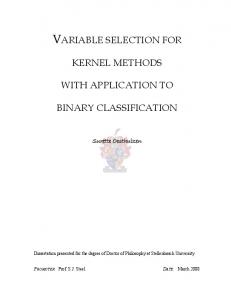
2.4.1 Kernel The term kernel has a long history. The meaning of the kernel depends on the subjects that has different meanings in different literatures. In mathematics, the term kernel itself is used with different meanings, for example, in linear algebra where it is used as a synonym for the null space. In the beginning of the last century David Hilbert and other researches, the term kernel has been used as a bivariate function to the field integral operators. The term kernel has been also used for density estimation in the statistical literature, where the kernel ∫ K : R → R is an integrable function satisfying K(x) dx = 1. The term kernel has been also used as a positive definite kernel (PDK) in the branch of mathematics since 1950s. The PDK is a large class of kernels, which contains Mercer kernel and so on. It can be regarded as a generalized dot product. Figure 2.1 presents the historical background of the kernel in the 20th century.
15
Functional Analysis and Kernel
Figure 2.1: Background of the kernel in the 20th century. Definition 2.4.1 (Kernel) Let X be a non-empty arbitrary set. A bivariate function k : X × X → R is called kernel on X if there exists a Hilbert space, H and a feature map Φ : X → H such that for all x, x′ ∈ X we have k(x, x′ ) = ⟨Φ(x), Φ(x′ )⟩.
16
Functional Analysis and Kernel In general the kernel may be also defined on the complex field. So, Hilbert space may be also a complex valued Hilbert space. Algorithms can be applied in dot product space by considering the kernel as a similarity measure. We can construct a kernel of several ways as follows: • straightforward construction of feature map and space, 2 • using a sequence of functions ( fn : X → F, n ∈ N such that ( fn (x))∞ n=1 ) ∈ ℓ , ∀x ∈ X,
• using algebraic properties of the set of kernels, k1 and k2 , – sum of kernels on same set (k1 + k2 ), – scalar multiplication of kernel (αk)< 0,
α ∈ F,
– product of kernel on different set, k1 k2 – polynomial of kernel with positive coefficients, – taking exponential, • using Taylor series, • using Fourier series, • pointwise limit of kernels. We can define a number of feature maps via a kernel as follows. • Aronszajn map: Φ : x → k(x, ·), Hk is the associated reproducing kernel Hilbert space (RKHS) k(x, y) = ⟨k(x, ·), k(y, ·)⟩. • Kolmogorov map: Φ : x → Xx , Hk = L2 (RX , µ), where µ is the Gaussian measure k(x, y) = E[Xx Xy ]. • Integral map: there exists a set T and a measure µ such that on has Φ : x → ∫ (Γ x (t))t∈T , Hk = L2 (T, µ), k(x, y) = Γ(x, t)Γ(y, t)dµ(t). • Basis map: given any orthonormal basis ( fα )α∈I of the RKHS associated with H, on ∑ has Φ : x → ( fα )α∈I , H = ℓ2 (I) and k(x, y) = α∈I fα (x) fα (y). When infinite sums are involved like in the Basis map, it is important to specify in which sense the sum converges. In general the convergence occurs for each pair. 17
Functional Analysis and Kernel
2.4.2 Advantages of kernel It is well-known that the feature space suffers the computational problem. In case of high dimensional data the computational cost becomes very high. Using inner product by the kernel we can overcome this problem efficiently. First advantage of the kernel is that in many important special case feature computation will be very inexpensive by k(x, z) = ⟨Φ(x), Φ(z)⟩, where x and z are in the arbitrary set X. Example 2.4.1 (Quadratic kernel) Let x, z ∈ Rm we have m m m ∑ m ∑ ∑ ∑ k(x, z) = [xT z]2 = ( xi zi )( x jz j) = (xi x j )(zi z j ) = ⟨Φ(x), Φ(z)⟩. i=1
j=1
i=1 j=1
In case m = 3 Φ(x) =
ϕ1 (x) ϕ2 (x) ϕ3 (x) ϕ4 (x) ϕ5 (x) ϕ6 (x) ϕ7 (x) ϕ8 (x) ϕ9 (x)
=
x1 x1 x1 x2 x1 x3 x2 x1 x2 x2 x2 x3 x3 x1 x3 x2 x3 x3
Cost for kernel, k(x, z) = O(m) is linear but for ϕ(x) = O(m2 ) is quadratic. Example 2.4.2 (Polynomial kernel) Let x, z ∈ Rm using polynomial kernel we have k(x, z) = [xT z + c]2 = ⟨x, z⟩2 + 2c⟨x, z⟩2 + c2 = ⟨Φ(x), Φ(z).⟩
18
Functional Analysis and Kernel In case m = 3 Φ(x) = In general dim(H) =
(m+d) d
ϕ1 (x) ϕ2 (x) ϕ3 (x) ϕ4 (x) ϕ5 (x) ϕ6 (x) ϕ7 (x) ϕ8 (x) ϕ9 (x) ϕ10 (x) ϕ11 (x) ϕ12 (x) ϕ13 (x)
=
x1 x2 x1 x3 x2 x1 x2 x2 x2 x3 x3 x1 x3 x2 x3 x3 √ 2cx1 √ 2cx2 √ 2cx3 c x1 x1
different features consisting all monomials having degree at
most d with input dimension m. The second advantage of the kernel is to use non-vectorial data, e.g., text strings or DNA sequences and so on. Another important advantage is that given a kernel we need neither the explicit form of the feature map nor the feature space, which are not also uniquely determined. Moreover, note that a similar construction can be made for arbitrary kernels and consequently every kernel has many different feature spaces. However, we can always construct a canonical feature space, namely the RKHSs (see Section 2.5). RKHSs have the remarkable and important property that norm convergence implies pointwise convergence.
2.4.3 Positive definite kernel (PDK) Although we have already seen several techniques to construct kernels, in general, we still have to find a feature space in order to decide whether a given function k is a kernel or not. Since this can sometimes be a difficult task, we will now present a criterion that characterizes R-valued kernels in terms of inequalities (positive semi-definite). By the
19
Functional Analysis and Kernel definition of positive definite function, if k is a R-valued kernel with feature map Φ : X → H. The kernel k is symmetric since the inner product in H is symmetric. Moreover, k is also positive definite since for n ∈ N, α1 , α2 , . . . , αn ∈ R and x1 , · · · , xn ∈ X n ∑ n ∑
αi α j k(xi , x j ) = ⟨
i=1 j=1
n ∑
αi Φ(xi ),
i=1
n ∑
α j Φ(x′j )⟩H ≥ 0.
j=1
We can check whether a bivariate function is PDK by symmetry and positiveness. Definition 2.4.2 (Kernel matrix or Gram matrix) Given a kernel k and inputs x1 , · · · , xn ∈ X, the square matrix K := (k(xi , x j ))i, j of order n is called the kernel matrix (Gram matrix) of k with respect to x1 , · · · , xn . Definition 2.4.3 (Positive semi-definite matrix) A real symmetric matrix K satisfying n n ∑ ∑
αi α j Ki j ≥ 0, ∀αi ∈ R
(2.2)
i=1 j=1
is called positive definite kernel. It is said to be strictly positive definite if equality in (2.2) occurs for α1 = α2 = · · · = αn = 0. Definition 2.4.4 (Positive definite kernel) A symmetric kernel k(·, ·) defined on a non-empty space X is called positive definite if for arbitrary number of points x1 , . . . , xn ∈ X the kernel matrix (k(xi , x j ))ni, j=1 is positive semi-definite. In kernel methods, the nonlinear feature map is given by a positive definite kernel, which provides nonlinear methods for data analysis with efficient computation. It is known that a positive definite kernel k is associated with a Hilbert space H, called reproducing kernel Hilbert space (see Section 2.5), consisting of functions on X so that the function value is reproduced by the kernel (Aronszajn, 1950). Definition 2.4.5 (Reproducing property) For any function of RKHS, i.e., f ∈ H and a point x ∈ X, the function value f (x) is given by f (x) = ⟨ f (·), k(·, x)⟩H , 20
(2.3)
Functional Analysis and Kernel where ⟨, ⟩H in the inner product of H, which is called reproducing property. The reproducing property says that each Dirac functional can be represented by the reproducing kernel. A Hilbert function space H that has a reproducing kernel k is always a RKHS (see Section 2.5). Every RKHS has a (unique) reproducing kernel and that this kernel can be determined by the Dirac functionals. Definition 2.4.6 (Kernel trick) By replacing f with k(·, x˜ ) in Eq. (2.3) yields k(x, x˜ ) = ⟨k(·, x), k(·, x˜ )⟩H for any x, x˜ ∈ X. To transform data for extracting nonlinear features, the feature map Φ : X → H is defined by Φ(x) = k(·, x), which is regarded as a function of the first argument. The inner product of two feature vectors is then given by ⟨Φ(x), Φ(˜x)⟩H = k(x, x˜ ). This is known as the kernel trick. The kernel trick serves as a central equation in the kernel methods. By this trick the kernel can evaluate the inner product of any two feature vectors efficiently without knowing an explicit form of neither Φ(·) nor H. With this computation of inner product, many linear methods of classical data analysis techniques can be extended to nonlinear ones with an efficient computation based on Gram matrices. Once Gram matrices are computed, the computational cost does not depend on the dimensionality of the original space.
2.4.4 Well-known PDKs and its parameters Assume k : X × X → R is positive definite kernel. Then for any x, x′ ∈ X, the following kernels are real valued positive definite kernels on R: 21
Functional Analysis and Kernel i. Linear kernel k0 (x, x′ ) = ⟨x, x′ ⟩ = xT x′ . It is just used the underlying Euclidean space to define the similarity measure. Whenever the dimensionality of x is very high, this may allow for more complexity in the function class than what we could measure and assess otherwise. It has limitation of linearity. ii. Polynomial kernel kP (x, x′ ) = (xT x′ + c)d , (c ≥ 0, d ∈ N). Using polynomial kernel it is possible to use the higher order correlation between the data in the different purposes. This kernel incorporates all polynomial interactions up to degree d (provided that c > 0). For instance, if we wanted to take only mean and variance into account, we would only need to consider d = 2 and c = 1. For higher emphasis on mean we need to increase the constant offset a. Polynomial kernels only map data into a finite dimensional space. Due to the finite bounded degree such kernel will not provide us with guarantees for a good dependency measure. iii. Gaussian radial basis function (RBF) kernel ′ 2
kG (x, x′ ) = e−s||x−x || , (s > 0). Many radial basis function kernels, such as the Gaussian RBF kernel map x into an infinite dimensional space. iv. Exponential kernel kE (x, x′ ) = e(αx
T x′ )
, (α > 0).
22
Functional Analysis and Kernel v. Laplacian kernel ′
kL (x, x′ ) = e−β∥x−x ∥ , (β > 0). • Binomial kernel: Let X := {x ∈ Rd : ∥x∥2 < 1} and α > 0. Then k(x, x′ ) := (1 − ⟨x, x′ ⟩)−α .
Table 2.1: Examples of well-known positive definite kernels and its parameters. Kernel k(x, x˜ ) Parameter Polynomial (⟨x, x˜ ⟩ + c)d c ≥ 0, d ∈ N 2 Gaussian RBF e−s||x−˜x|| s>0 (αxT x˜ ) Exponential e α>0 −β∥x−˜x∥ Laplace e β>0
Definition 2.4.7 (Stationary kernels) Let κ : Rn → R be a function. Then κ is called a positive definite function (or function of positive type or Stationary kernels) if k(x, z) = κ(x − z) this type of the kernel is called stationary, a stationary kernel. It depends only on the lag vector separating the two examples x and z but not on the examples themselves. A stationary kernel of the form ϕ(x−y) is also called a shift invariant (or translation invariant) kernel. Gaussian and Laplacian kernels are example of stationary kernel. Definition 2.4.8 (Nonstationary kernels) A kernel is called nonstatinary, which depends on explicitly on the two examples x and z of k(x, z) . For example Linear kernel and polynomial kernel.
23
Functional Analysis and Kernel
2.4.5 Valid PDKs and its matrices Given an arbitrary set X. Assume there exist Φ such that k(x, x′ ) = ⟨Φ(x), Φ(x′ )⟩ (kernel trick) is a valid PDK, where x , x′ ∈ X. Let x1 , x2 , . . . , xn ∈ X and c1 , c2 , . . . , cn ∈ R. Then n ∑ n ∑
ci c j k(xi , x j ) =
n ∑ n ∑
i=1 j=1
ci c j ⟨Φ(xi ), Φ(x j )⟩ = ⟨
i=1 j=1
n ∑
ci Φ(xi ),
i=1
n ∑
c j Φ(x) j ⟩ = ||
i=1
n ∑
ci Φ(xi )||2 ≥ 0
i=1
i.e. the symmetric matrix
K = (k(xi , x j ))ni, j=1
k(x1 , x1 ) k(x1 , x2 ) k(x2 , x1 ) k(x2 , x2 ) = .. .. . . k(xn , x1 ) k(xn , x2 )
. . . k(x1 , xn ) . . . k(x2 , xn ) .. ... . . . . k(xn , xn )
is positive semidefinite. The kernel matrix K = (k(xi , x j ))ni, j=1 is often called a Gram matrix in statistical machine learning literature. Symmetry an positive definiteness are not only necessary for k to be a PDK but also sufficient. We do not actually need to have a centered Φ but for some methods we do need K ∑ 1∑ ˜ i j = ⟨Φ(x ˜ i ), Φ(x ˜ j )⟩ = ⟨Φ(xi ) − 1 K Φ(xa ), Φ(x j ) − Φ(xb )⟩ n a=1 n b=1 n n n n 1∑ 1 ∑∑ 1∑ = ⟨Φ(xi ), Φ(x j )⟩ − ⟨Φ(Xa ), Φ(x j )⟩ + 2 ⟨Φ(xa ), Φ(xb )⟩ ⟨Φ(xi ), Φ(xb )⟩ − n b=1 n a=1 n a=1 b=1 n n n n 1 ∑∑ 1∑ 1∑ = Ki j − Kib − Ka j + 2 Kab n b=1 n a=1 n a=1 b=1 n n n n 1∑ 1∑ 1 ∑∑ 1ia Kab 1b j = Ki j − Kib 1b j − 1ia Ka j + 2 n b=1 n a=1 n a=1 b=1 n
n
= (K − K(n−1 Jn ) − (n−1 Jn )K + (n−1 Jn )K(n−1 Jn ))i j , = (HKH)i j
(2.4)
where for all i and j, 1i j = 1, 1n = [1, 1, · · · , 1]T , and H = In − 1n Jn with Jn = 1n 1Tn .
24
Functional Analysis and Kernel The centered vector of a test point x is defied as ˜ x1 ), · · · , k(x, ˜ x1 )]T k˜ x = [k(x, 1 1 1 = kx − Jn kx − K1n + 2 Jn K1n n n n 1 = H[kx − K1n ], n where kx = [k(x, x1 ), · · · , k(x, xn )]T . Given a set of test points xt1 , · · · xtL , as in Eq. (2.1), we can define the centered matrix of order L × n, ∑ 1∑ ˜ t = ⟨Φ(xti ) − 1 Φ(xb )⟩ K Φ(xa ), Φ(x j ) − n a=1 n b=1 n
n
in terms of the non centered matrix Kt = ⟨Φ(xti ), Φ(x j )⟩, we have
˜ t = Kt − 1 JTL×n K − 1 Kt JL×n + 1 JTL×n K 1 JL×n , K n n n 2 where JL×n is the L × n matrix with all entries equal to 1. A good monograph on the theory of positive definite kernels is Steinwart and Christmann, 2008 (Steinwart and Christmann, 2008, Chapter 4). The following sections all unspecified results are taken from that work. Theorem 2.4.1 For any set X , ∅ and a real valued function k : X × X → R is a PDK, i.e., it is symmetric and positive semi-definite, if and only if there is a mapping Φ : X → H with a scalar product ⟨·, ·⟩ such that k(x, x′ ) = ⟨Φ(x), Φ(x′ )⟩,
∀x, x′ ∈ X.
Theorem 2.4.2 Let X be a non-empty set and fn : X → F, n ∈ N, be functions such that 2 ( fn (x))∞ n=1 ∈ ℓ for all x ∈ X. Then
′
k(x, x ) :=
∞ ∑
fn (x) fn (x′ ),
n=1
25
∀x′ ∈ X,
(2.5)
Functional Analysis and Kernel defines a PDK on X. Definition 2.4.9 (Restriction of PDK) Let k is a kernel on X, X˜ be a set, and L : X → X˜ be a map. Then k˜ defined by ˜ x′ ) := k(L(x), L(x′ )), k(x,
∀x, x′ ∈ X,
˜ In particular, if X˜ ⊂ X, then k|X× is a PDK on X. ˜ X˜ is a PDK.
2.4.6 Properties of PDKs Theorem 2.4.3 Let k : X × X → C be a PDK, Hc be a C-Hilbert space, and Φ : X → Hc be a feature map of k. Assume that we have k(x, x′ ) ∈ R for all x, x′ ∈ X. Then Hr = Hc equipped with the inner product ⟨z, z′ ⟩Hr := Re⟨z, z′ ⟩Hc ,
z, z′ ∈ Hr ,
is an R-Hilbert space, and Φ : X → Hr is a feature map of k. Theorem 2.4.4 Let X be a set, α ≥ 0, and k, k1 , and k2 be PDKs on X. Then αk and k1 + k2 are also PDKs on X. The preceding theorem 2.4.4 states that the set of PDKs on X is a cone. It is, however, not a vector space since, in general differences of PDKs are not a PDK. Theorem 2.4.5 Let k1 be a PDK on X1 and k2 be a PDK on X2 . Then k1 · k2 is a PDK on X1 × X2 . In particular, if X1 = X2 , then k(x, x′ ) := k1 (x, x′ )k2 (x, x′ ), x, x′ ∈ X, defines a PDK on X. With the above two theorems, (2.4.4 and 2.4.5) it is easy to construct the non-trivial kernels. To illustrate this, let us assume for simplicity that X = R. Then for every integer n ≥ 0, the map kn defined by kn (x, x′ ) := (xx′ )n , ∀x, x′ ∈ X
26
Functional Analysis and Kernel is a PDK by the 2.4.2. Consequently, if p : X → R is a polynomial of the for p(t) = a0 + a1 t + . . . + am tm with non-negative coefficients ai , then k(x, x′ ) := p(xx′ ),
x, x′ ∈ X
(2.6)
is define a PDK on X by theorem (2.4.4). Theorem 2.4.6 Let p ≥ 0 and d ≥ 0 be integers and c ≥ 0 be a real number. Then k defined by k(z, z′ ) := (⟨z, z′ ⟩ + c) p , z, z′ ∈ Cd , is a kernel on Cd . Moreover, its restriction to Rd is a R-valued PDK. Note that the polynomial kernel defined by p = 1 and c = 0 are called a linear kernel. Instead of using polynomials for constructing kernels, one can use functions that can be represented by Taylor series. This is done in the following theorem. Theorem 2.4.7 (Taylor type kernel) Let ÅC and ÅCd be the open unit balls of C and Cd , respectively . Moreover, let r ∈ (0, ∞) and f : rÅC → C be holomorphic with Talylor series f (z) =
∞ ∑
an zn , z ∈ ÅC
n=0
If an ≥ 0 for all n ≥ 0, then
′
′
k(z, z ) := f (⟨z, z ⟩Cd ) =
∞ ∑
an ⟨z, z′ ⟩nCd ,
z, z′ ∈
√
rÅCd ,
n=0
defines a kernel on
√
rÅCd whose restriction to X = {x ∈ Rd : ∥x∥2
0 is given by k s,Cd (z, z′ ) := e−s 27
∑d
z′j )2 j=1 (z j −¯
,
Functional Analysis and Kernel where d ∈ N and z, z′ ∈ Cd . If we make a restriction k s := (k s,Cd )|Rd ×Rd is an R-valued kernel, which we call the (real) Gaussian RBF kernel with width s. Obviously, this kernel satisfies ′ 2
k s (x, x′ ) := e−s||x−x ||2 ,
∀x, x′ ∈ R,
where || · || denotes the Euclidean norm on Rd . Definition 2.4.10 (A family of spaces) Let s > 0 and d ∈ N. For a given holomophic function f : Cd → C we define (
|| f || s,Cd
2d s2d := πd
∫ C
d
2 −s2
| f (z)| e
∑d
z′j )2 j=1 (z j −¯
) ,
whee dz stands for the complex Lebesgue measure on Cd . Furthermore, we write { } H s,Cd := f : Cd → C f holomorphic and || f || s,Cd < ∞ . Example 2.4.4 (RBF kernel) By considering RBF kernel k(x, z) = e− 2s2 ||x−z|| 1
2
= e− 2s2 ⟨x,x⟩ e s2 ⟨x,z⟩ e− 2s2 ⟨z,z⟩ [ ] ⟨x, z⟩ 1 ⟨x, z⟩2 − 12 ⟨x,x⟩ − 12 ⟨z,z⟩ 2s = e 2s 1+ 2 + + . . . e s 2! (s2 )2 ∞ ∑ 1 ⟨x, z⟩i − 1 ⟨z,z⟩ − 12 ⟨x,x⟩ = e 2s e 2s2 2 )i i! (s i=0 ∞ ∑ 1 − 12 ⟨x,x⟩ xi zi − 12 ⟨z,z⟩ = e 2s e 2s i (s)i i! (s) i=0 1
1
1
= ⟨Φ(x), Φ(z)⟩, where ϕ1 (x) ϕ2 (x) 1 , ϕi (x) = e− 2s2 ⟨x,x⟩ 1 xi . Φ(x) = i!si ϕ3 (x) .. .
28
Functional Analysis and Kernel Definition 2.4.11 (Fourier type kernel) Let f : [−2π, 2π] → R be a continuous function that can be expanded in a pointwise convergent Fourier series of the form f (t) =
∞ ∑
an cos(nt).
n=0
If an ≥ 0 holds for all n ≥ 0 then k(x, x′ ) :=
∏d i=1
f (xi − x′i ) defines a kernel on [0, 2π)d . We
say that k is a PDK of Fourier type. Theorem 2.4.8 Assume k : X × X → R is positive definite and x, y ∈ X, 1. Positive definiteness implies positivity on the diagonal k(x, x) ≥ 0 2. Cauchy- Schwarz inequality |k(x, y)|2 ≤ k(x, x)k(y, y) Proof 2.4.1 Positive definiteness implies positive on the diagonal and symmetry i.e. k(x, y) = k(y, x). The 2 × 2 gram matrix with entries Ki j = k(xi , x j ) is positive. With fact k(xi , x j ) = k(x j , xi ), the definition of positive definiteness implies that the eigenvalues of the hermitian matrix k(x , x ) k(x , x ) 1 1 1 2 k(x2 , x1 ) k(x2 , x2 )
k(x , x ) k(x , x ) 1 1 2 1 = k(x2 , x1 ) k(x2 , x2 )
is non-negative, thus its determinant k(x1 , x1 )k(x2 , x2 ) − |k(x1 , x2 )|2 i.e., 0 ≥ K11 K22 − K12 K21 = K11 K22 − K12 K12 = K11 K22 − |K12 |2 Theorem 2.4.9 (Limits of PDKs are alos a PDK) Let (kn ) be a sequence of PDKs on the set X that converges pointwise to a function k : X × X → R, i.e., limn→∞ kn (x, x′ ) = k(x, x′ ) for all x, x′ ∈ X. Then k is a PDK on X. To prove we need to show k is symmetric and positive definite.
29
Functional Analysis and Kernel For any PDK, via space Φ, H so that kernel trick holds: f (·) =
m ∑
αi k(·, xi ),
g(·) =
n ∑
i=1
β j k(., x j ),
⟨ f, g⟩H =
j=1
∑∑
αi β j k(xi , x j ),
i=1 j=1
where m, n ∈ N, αi , β j ∈ R and xi , x j ∈ X • Symmetry: ∑∑
⟨ f, g⟩ =
αi β j k(xi , x j ) =
i=1 j=1
∑∑
αi β j k(x j , xi ) = ⟨g, f ⟩.
i=1 j=1
• Bilinearity: ⟨ f, g⟩ =
∑∑
αi β j k(xi , x j ) =
i=1 j=1
∑
β j f (x j ) =
j=1
∑
αi g(xi ).
i=1
• Non-negative: ⟨ f, f ⟩ =
∑∑
αi α j k(xi , x j ) ≥ 0.
i=1 j=1
Let us see what happens if we evaluate the inner product of f ∈ H with k(·, xi ) ⟨k(·, x), f (·)⟩ =
n ∑
αi ⟨k(·, x), k(·, x j )⟩ =
n ∑
αi ⟨k(x, x j )⟩ = f (x).
(2.7)
i=1
i=1
The above reproducing property, together with the Cauchy-Schwartz inequality |⟨x, y⟩| ≤ ||x||||y||, implies that: | f (x)|2 = |⟨k(·, x), f ⟩|2 ≤ ⟨k(·, x), k(·, x)⟩⟨ f, f ⟩ which in turn implies that f = 0 if ⟨ f, f ⟩ = 0. Thus the vector space of feature map Φ(x) = k(·, x) induces with (2.7) k(x, z) = ⟨Φ(x), Φ(x′ )⟩H , H as simply a pre-Hilbert space. To make it a true Hilbert space we must take its 30
Functional Analysis and Kernel closure, including the set of all limit points for sequences in H defined with respect to some (induced) norm.
2.4.7 Interplay between PDK, reproducing kernel and Mercer kernel A kernel can be also defined on the functional viewpoint since each PDK k on a set X is associated a Hilbert space Hk of real-valued functions on X. Definition 2.4.12 (Reproducing kernel) Let X be a non-empty arbitrary set. A bivariate function k : X × X → R is called reproducing kernel a Hilbert space H on X iff i) for all elements of X, the function k will be in H i.e., ∀x ∈ X,
k(·, x) ∈ H,
ii) the function k follows reproducing property. Due to Moore Aronszajn theorem (Aronszajn, 1950), it can be shown that the definition of positive definite kernel and reproducing kernel are equivalent. Proposition 2.4.1 The reproducing kernel k(·, x) of a reproducing kernel Hilbert space Hk is a positive matrix. Proof 2.4.2 Let us assume, kx (·) = k(·, x) be the a reproducing kernel Hilbert space Hk . We have 0 ≤ ||
n ∑
αi kxi ||
2
=
n ∑
αi k x i , i=1 j=1 n n ∑∑
= ⟨
i=1
n ∑
α j kx j ⟩ =
n n ∑ ∑
αi αi ⟨kxi , kx j ⟩
i=1 j=1
αi αi k(xi , x j ).
i=1 j=1
Hence n ∑ n ∑
αi αi k(xi , x j ) ≥ 0.
i=1 j=1
Theorem 2.4.10 (Moore Aronszajn, 1950) Let k : X×X → R be a positive definite kernel on a set X. Then, there uniquely exists a RKHS Hk on X such that 31
Functional Analysis and Kernel • k(·, x) ∈ Hk , ∀x ∈ X. • The subspace H of Hk and H= Span{k(·, x) : x ∈ X} is dense in Hk . • k is the reproducing kernel on Hk , i.e., f (x) = ⟨ f, k(·, x)⟩Hk , (∀x ∈ X, ∀ f ∈ Hk ). • Hk is the set of functions on X which are pointwise limits of Cauchy sequence in H with the inner product ⟨ f, g⟩ =
∑∑
αi β j k(xi , x j )⟩,
i=1 j=1
where f (·) =
m ∑
αi k(·, xi )
and
g(·) =
n ∑
β j k(·, x j ).
j=1
i=1
The above theorem tells us one-to 0ne correspondence between PDK and RKHS i.e., k ⇔ Hk . Theorem 2.4.11 (Mercer (1909)) Let X ⊂ Rn , n ∈ N be closed, a strictly positive and finite Borel measure ν on X and a continuous k : X × X → R satisfying: for any finite of N N points {xi }i=1 in X and real numbers {ai }i=1
N ∑ N ∑
ai a j k(xi , x j ) ≥ 0,
i=1 j=1
and ∫ ∫ X
X
k(x, x′ )2 dν(x)dν(x′ ) < ∞.
32
Functional Analysis and Kernel Let Lk : Lν2 (X) → Lν2 (X) be a integral operator defined as ∫ Lk f (x) =
X
k(x, x′ ) f (x′ )dν(x′ ), f ∈ L2 (ν)
with a countable system of nonnegative eigenvalues {µi }∞ i=1 satisfying
∑∞
i=1
µ2i < ∞ and
corresponding orthonormal eigenfunctions (ei )∞ i=1 . Then ′
k(x, x ) =
∞ ∑
µi ei (x)ei (x′ ), x, x′ ∈ X,
(2.8)
i=1
where the convergence is absolute for each pair (x, x′ ) ∈ X × X and uniform on each compact subset of X. We can define the feature map via the Mercer’s theorem as follows √ eν : X → ℓ2 , eν (x) = ( λi ei (x))∞ i=1 , where if only N < ∞ of the eigenvalues are strictly positive, then eν : X → RN . The notion of positive definite kernel was not well-known before the 1950s. Instead, researchers have been used kernels that satisfy the conditions of Mercer’s theorem, called Mercer’s kernel. A kernel which satisfied the conditions of Mercer’s theorem implies that the kernel also satisfied the kernel trick i.e., k(x, x′ ) = ⟨Φ(x), Φ(x′ )⟩ but the converse is not true. So all Mercer’s kernels are PDKs but all PDKs are not Mercer’s kernels. Mercer’s theorem is a special case of the basis map. It gives a stronger (uniform) convergence properties of the kernel representation, but needs additional assumption, namely X has to be compact and the kernel is continuous. Mercer’s theorem has played a crucial role in supervised learning, say SVM in which the kernel trick is introduced via Mercer’s theorem.
2.5 Reproducing kernel Hilbert space (RKHS) It is known (Aronszajn, 1950) that a positive definite kernel k is associated with a Hilbert space H, called reproducing kernel Hilbert space (RKHS), consisting of functions on X so that the function value is reproduced by the kernel.
33
Functional Analysis and Kernel Definition 2.5.1 (Reproducing kernel Hilbert spaces) Let a set X , ∅. A RKHS of a kernel k, Hk over X is a space of functions f : X → R such that • The function k is defined as k : X × X → R. • For every x ∈ X and f ∈ Hk f (x) = ⟨ f (·), k(·, x)⟩Hk . where kx = k(·, x) ∈ Hk is a function with fixed x (k has reproducing property). • Hk = span{k(·, x) : x ∈ X} i.e., k spans Hk , where A denotes the completion set of A. The Reproducing kernel Hilbert spaces (RKHS) of a PDK are in a certain sense the smallest feature space of this PDK and consequently can serve as a canonical feature space. Now, we briefly discuss the properties of RKHS.
2.5.1 Properties of RKHS Reproducing kernel Hilbert spaces have the remarkable and important property that norm convergence implies pointwise convergence. More precisely, let H be a RKHS, f ∈ Hk , and ( fi )∞ i ⊂ Hk be a sequence with ∥ fn − f ∥H → 0 for i → ∞ (there is a convergence sequence). Then for all x ∈ X, we have lim fn (x) = lim δx ( fn ) = f (x).
n→∞
n→∞
Reproducing kernels are actually kernels since the feature map is defined by the kernels. The reproducing property says that each Dirac functional can be represented by the reproducing kernel. Consequently, a Hilbert function space that has a reproducing kernel is always a RKHS. Every RKHS has a (unique) reproducing kernel and this kernel can be determined by the Dirac functional. Theorem 2.5.1 Let Hk be a Hilbert function space over X with a reproducing kernel k. Then Hk be a RKHS over X and Hk is also a feature space of k, where the feature map
34
Functional Analysis and Kernel Φ : X → Hk is defined as Φ(x) = k(·, x), ∀x ∈ X. Theorem 2.5.2 Let Hk be a RKHS over X. Then k : X × X → K defined by k(x, x′ ) := ⟨δx , δx′ ⟩, ∀x, x′ ∈ X, is the only reproducing kernel on Hk . Furthermore, if (ei )i∈I is an orthonormal basis (ONB) or complete orthonormal system of Hk then for all x, x′ ∈ X, we have k(x, x′ ) =
∑
ei (x)ei (x′ ),
(2.9)
i∈I
where the convergence is absolute. The theorem 2.5.2 tells us, a RKHS uniquely determines its reproducing kernel, which is actually a kernel. The ONB in the theorem2.5.2 is not necessarily countable. However, RKHSs over separable metric spaces having a continuous kernel are always separable and hence all their ONBs are countable. In particular, the RKHSs of Gaussian RBF kernels always have countable ONBs. A non separable Hilbert space of continuous functions on a separable topological space has no reproducing kernel. Theorem 2.5.3 Let X , 0 and k be a kernel over X with the feature space H and feature map Φ : X → H. Then Hk := {⟨w, Φ(·)⟩H : w ∈ H}
(2.10)
|| f ||Hk := inf {||w||H : w ∈ H with f = ⟨w, Φ(·)⟩H }
(2.11)
equipped with the norm
is the only RKHS of k. In particular both definitions are independent of the choice of H
35
Functional Analysis and Kernel and Φ0 and the operator V : H → Hk defined by Vw := ⟨w, Φ(·)⟩H , w ∈ H is a metric surjection, i.e., VÅH = ÅHk , where ÅH and ÅHk are the open unit balls of H and Hk , respectively. Observations on the theorem 2.5.3: the RKHS Hk of a given kernel k as the “smallest” feature space of k in the sense that there is a canonical metric surjection V from any other feature space H0 of k onto Hk . The soft margin SVM produce decision functions of the form x → ⟨w, Φ(x)⟩, where Φ : X → Hk is a feature map of k and w ∈ Hk is a suitable weight vector. Now, (2.10) states that the RKHS associated with k consists exactly of all possible functions of this form. Moreover, (2.10) shows that this set of functions does not change if we consider different feature spaces or feature maps of k. The Theorem 2.5.3 can often be used to determine the RKHS of a given kernel and its modifications such as restrictions and normalization. To illustrate this let us recall that every C-valued kernel on X that is actually R-valued has an R-feature space. Corollary 2.5.1 Let k : X × X → C be a kernel and Hk its corresponding C-RKHS. If we actually have k(x, x′ ) ∈ R, then { } HkR := inf f : X × X → R ∃g ∈ Hk with Re g = f , equipped with the norm { } || f ||HkR := inf ||g||Hk : g ∈ Hk with Re g = f ,
f ∈ HkR ,
is the R-RKHS of the R-valued kernel k. Given a RKHS, Hk and its kernel k(x, y) on X, then for all x, y ∈ X: • k(x, x) ≥ 0 • k(y, x) = k(x, y) • |k(y, x)|2 ≤ k(y, y)k(x, x) 36
Functional Analysis and Kernel • Let x0 ∈ X. Then the following are equivalent: – k(x0 , x0 ) = 0. – k(y, x0 ) = 0, ∀y ∈ X. – f (x0 ) = 0, ∀ f ∈ H.
2.5.2 Representer theorem Representer theorem implies optimizer is the linear combination of kernels subject to the sample points Theorem 2.5.4 (Kimeldorf and Wahba (1971)) Let x1 , x2 , · · · , xn ∈ X and Hk be a reproducing kernel Hilbert space with a kernel k : X × X → R, a symmetric positive semi-definite function of the compact domain. For any function L : Rn → R and any nondecreasing function Ω : R → R. If J ∗ = min J( f ) = min {Ω(|| f ||H ) + L( f (x1 ), . . . f (xn ))} f ∈H
f ∈H
is well-defined, then there are some α1 , α2 , . . . , αn ∈ R, such that f (·) =
n ∑
αi k(·, xi )
i=1
achieves J( f ) = J ∗ . Further more if Ω is increasing, then each minimizer of J(f) can be ∑ expressed in the form f (·) = ni=1 αi k(·, xi ). Example 2.5.1 Let X be a set and (e1 , e2 , . . . , en ) be an orthonormal basis in H also define ′
k(x, x ) =
n ∑
ei (x)ei (x′ ).
i=1
Then for any x′ ∈ X k(·, x′ ) =
n ∑
ei (x′ )ei (·)
i=1
37
Functional Analysis and Kernel belongs to Hk and for any function φ(·) =
n ∑
λi ei (·)
i=1
in H, we have ′
′
∀x ∈ X, ⟨φ, k(·, x )⟩H = ⟨
n ∑
λi ei (·),
i=1
=
n ∑ n ∑
n ∑
e j (x′ )e j (·)⟩H
j=1
λi e j (x′ )⟨ei (·), e j (·)⟩H
i=1 j=1
=
n ∑
λi ei (x′ ) = φ(x′ )
i=1
Any finite dimensional Hilbert space of functions has a reproducing kernel. Example 2.5.2 Let k(i, j) = δi j (delta function or Kronecker symbol, equal to 1 if i = j and 0 otherwise). Then
∀ j ∈ N, k(·, j) = (0, 0, . . . , 1, . . . , 0) ∈ H ∀ j ∈ N, ∀x = (xi )i∈N ∈ H, ⟨x, k(·, j)⟩H =
∑
(1 at the jth place) xi δi j = x j .
(2.12)
i∈N
k is the reproducing kernel of H.
2.6
Methods based on RKHS
The kernel based methods are developed by combining the kernel trick and representer theorem, i.e., Kernel trick + Representer theorem = Foundation of kernel methods. A number of kernel methods have been proposed as in the supervised learning, in unsupervised learning, in nonparametric inference and so on.
38
Functional Analysis and Kernel
2.6.1 Supervised learning Supervised learning is the main and well-know first type of machine learning. It consists of input-output pairs. For given a labeled set of input-output pairs D = {(Xi , Yi )}ni=1 , the goal of supervised learning is to learn a function, f : X → Y, where D is a training set with n training data points. The useful supervised kernel methods on RKHS are as follows: • Support vector machine for classification (SVM, Boser et al., 1992). • Support vector machine for regression (Smola and Sch¨olkopf, 1998). • Kernel ridge regression (Saunders et al., 1998).
2.6.2
Unsupervised learning
Unsupervised learning, knowledge discovery is the second main type of machine learning. It consists of only input data and arguably more typical of human learning. For given an input D = {(Xi )}ni=1 the goal of unsupervised methods are to discover interesting structure in the data where D is a training set with n data points. Useful unsupervised kernel methods of RKHS are as follows: • Kernel principal component analysis (Sch¨olkopf et al., 1998) . • Kernel canonical correlation analysis (Akaho, 2001). • Kernel K-mean cluster analysis (Kim et al., 2005). • Gradient-based kernel dimension reduction for regression (Fukumizu and Leng, 2014).
2.6.3 Nonparametric inference Nonparametric inference methods on RKHS are the recent developed kernel methods. Nonparametric inference aims to identify very general processes from the data. The useful kernel methods of nonparametric inference are as follows: • Bayesian inference with positive definite kernels (Fukumizu et al., 2013). • Kernel two-sample test (Gretton, 2012). 39
Chapter 3 Automatic Way of Finding Hyperparameters in Kernel Principal Component Analysis 3.1 Motivation Dimension reduction is an essential part of modern data analysis, where we often need to handle large dimensional data. The purpose of dimension reduction may be visualized, noise reduction, and pre-processing for further analysis. Among others, the principal component analysis (PCA, Pearson, 1901) is one of the most famous methods to reduce the dimensionality by projecting data onto a low-dimensional subspace with largest variance. Kernel principal component analysis (kernel PCA, Sch¨olkopf et al., 1998) has been proposed as a nonlinear extension of the standard PCA, and has been applied to various purposes including feature extraction, denoising, and pre-processing of regression. Kernel PCA is an example of the so-called kernel methods (Sch¨olkopf and Smola, 2002), which aim to extract nonlinear features of the original data by mapping them into a highdimensional feature space (reproducing kernel Hilbert space, RKHS). This mapping is called feature map. A number of methods have been proposed as kernel methods, which include support vector machine (SVM, Boser et al., 1992), a novel multiclass SVM algorithm using mean reversion and coefficient of variance (Premanode et al., 2013), kernel ridge regression (Saunders et al., 1998), kernel canonical correlation analysis (Akaho,
Automatic Way of Finding Hyperparameters in kernel PCA 2001, Bach and Jordan, 2002), Bayesian Inference with Positive Definite Kernels (Fukumizu et al., 2013), Gradient-Based Kernel Dimension Reduction for Regression (Fukumizu and Leng, 2014) and so on. It is well known that the performance of a kernel method is highly dependent on the choice of the kernel. For supervised learning such as SVM and kernel ridge regression, cross-validation is popularly used for choosing the hyperparameters of a kernel algorithm, such as parameters in a kernel (e.g., bandwidth of Gaussian RBF kernel), with the objective function of learning. On the other hand, no well-founded methods have been proposed in general for unsupervised learning such as kernel PCA and kernel canonical correlation analysis. This chapter focuses on kernel PCA and proposes a method for choosing hyperparameters: parameters in a kernel and the number of kernel principal components. In the case of standard linear PCA, the algorithm can be formulated as minimization for self-regression with reduced rank, and cross-validation approaches have been proposed for choosing the number of components (Krzanowski, 1987, Wold, 1978). In contrast, while a similar regression formulation is possible for kernel PCA, the cross-validation approach is not applicable straightforwardly for choosing a kernel in kernel PCA: the error of the regression is given by the RKHS norm of the feature space associated with the kernel, and thus the cross-validation errors are not comparable for different kernels. As detailed in Section 3.2, the proposed method for choosing the hyperparameters of kernel PCA uses cross-validation for the reconstruction errors of pre-images in the original space. The pre-image of a feature vector is defined by an approximate inverse image of the feature map (Mika et al., 1999). Various methods have been already proposed to calculate the pre-image of a feature vector, as explained in Section 3.2.1 (Mika et al., 1999, Kwok and Tsang, 2003, Bakir et al., 2004, Rathi et al., 2006, Arias et al., 2007, Zheng et al., 2010). In the proposed method, given an evaluation data in the cross-validation, we compute the pre-image of the corresponding feature vector projected onto the subspace given by kernel PCA, and then evaluate the reconstruction error of the evaluation point. A kernel and the number of components corresponding to the minimum average reconstruction error are chosen as the optimum ones. We demonstrate the effectiveness of this method experimentally with various synthesized and real-world datasets.
41
Automatic Way of Finding Hyperparameters in kernel PCA
3.1.1
Kernel principal component analysis (kernel PCA)
Kernel PCA (Sch¨olkopf et al., 1998) conducts principal component analysis for the feature vectors. More precisely, given data points Xi ∈ X, i = 1, 2, . . . , n, kernel PCA outputs a set of principal functions by the following two-step procedure: (i) transform the data nonlinearly into the feature space H, i.e., Xi 7→ Φ(Xi ), (ii) solve the linear PCA problem for the feature vectors, i.e., solve the directions in H for which the variance of {Φ(Xi )} along those directions is maximized. The algorithm of kernel PCA is described as follows (for the detail, see Sch¨olkopf et al. ∑ ˜ (1998)). Let Φ(X) := Φ(X) − 1n nj=1 Φ(X j ) be the centered feature vector. The estimated ∑ ˜ T ˜ covariance matrix is given by H = 1n ni=1 Φ(X i )Φ(Xi ) with the centered feature vectors. The principal directions g ∈ H are given by the unit eigenvectors corresponding to the largest eigenvalues, and thus the problem is converted to solving the eigenequation ˜ Hg = λg. By using the kernel trick, this problem is reduced to the generalized eigen value problem ∑ ˜ i ) such that that finds g = ni=1 αi Φ(X ˜ Mα = nλα,
subject to
αT Mα = 1,
(3.1)
where M is the n × n centered Gram matrix defined by M = CKC with Ki j = k(Xi , X j ) and C = In − n1 1n 1Tn . Here In is the identity matrix of size n, and 1n is the vector with n ones. The constraint αT Mα = 1 corresponds to the condition ⟨g j , gh ⟩ = δ jh , where δ jh is the Kronecker’s delta. Let λ1 ≥ λ2 ≥ . . . ≥ λn ≥ 0 denote the ordered eigenvalues of M with associated eigenvectors α1 , . . . αn , where α j = (α1 j . . . αn j )T . The vectors are normalized so that αTj Mαh = δ jh . The j-th principal direction g j ∈ H is then given by n 1 ∑ ˜ i ), gj = √ αi j Φ(X λ j i=1
42
Automatic Way of Finding Hyperparameters in kernel PCA and the j-th principal component of the data point Xi is given by √ ˜ i )⟩ = √1 (Mα j )i = λ j αi j . ⟨g j , Φ(X λj For a test point X out of the sample, the j-th principal component is similarly given by n 1 ∑˜ ˜ k(X, Xi )αi j , ⟨g j , Φ(X)⟩ = √ λ j i=1
˜ y) = k(x, y) − 1 ∑ni=1 k(x, Xi ) − 1 ∑ni=1 k(Xi , y) + 12 ∑ni, j=1 k(Xi , X j ) is the centered where k(x, n n n kernel.
3.1.2 Choice of kernel The result of kernel PCA obviously depends on the choice of the kernel. It is often the case that the kernel has some parameters like the popular examples shown in Table 2.1. In such a case, these parameters may have a strong influence on the results. To depict the influence, using wine data (see Section 3.3) we show the plots of the first two kernel principal components with different values of inverse-bandwidth parameter s in the Gaussian RBF kernel, and degree d and constant c in the polynomial kernel (Figure 3.2). From the figure, we see that in both the kernels the results of kernel PCA depend strongly on the parameters, and an appropriate choice is indispensable for the method to give reasonable low-dimensional representation of data. It is known that the standard PCA can be formulated as a self-regression or reconstruction problem; namely, the first r principal components of centered data {Xi }ni=1 ⊂ Rd are equal to the projections BXi given by the reduced rank regression min A,B
n ∑
∥Xi − ABXi ∥2
subject to BBT = Ir ,
i=1
where A and B are d × r and r × d matrices, respectively. Based on this regression formulation, the cross-validation approach (Stone, 1974) has been used for the standard PCA to choose the number of components (Wold, 1978, Krzanowski, 1987) by minimizing the above self-regression errors.
43
Automatic Way of Finding Hyperparameters in kernel PCA
H r 1 K
Feature Spaces rH2
r H3
P C k1
A
k2
k3
Input Space Figure 3.1: Individual reproducing kernel Hilbert space for each kernel of the kernel principal component analysis (KPCA). In a similar manner, the kernel PCA can be also formulated as the self-regression of the centered feature vectors. In fact, it is easy to see that the first r principal directions are given by
min
f j ,g j ∈H
n r
2 ∑ ∑
˜
˜ f ⟨g , Φ(X )⟩ Φ(X ) −
j j i , i H i=1
j=1
where f j , g j ∈ H with ⟨g j , gℓ ⟩H = δ jℓ . One might expect that this self-regression formulation could be applied to the cross-validation method for choosing a kernel in kernel PCA. This is not possible, however, because the above regression error is measured by the RKHS norm given by the kernel, and thus the errors are not comparable among different kernels. This problem is shown in the Figure 3.1. The goal of this chapter is thus to propose a method of choosing a kernel (and the number of components) in kernel PCA by introducing a criterion comparable for different kernels (Alam and Fukumizu, 2014).
44
Automatic Way of Finding Hyperparameters in kernel PCA
Figure 3.2: Scatter plots of the first two kernel principal components for wine data: Gaussian RBF kernel is used in the top panel (a) s = 0.05 (b) s = 0.75 (c) s = 1 (d) s = 10, and polynomial kernel in the bottom (e) c = 0.001, d = 2 (f) c = 10, d = 2 (g) c = 1, d = 3 (h) c = 1, d = 4.
3.2
Proposed methods
The proposed method for choosing a kernel and the number of component uses crossvalidation by the comparable reconstruction errors in the original space. To evaluate the errors, we need to solve the pre-image of the feature vectors projected on the subspace given by the principal directions. We first give a brief review of pre-image methods.
3.2.1 Pre-Image of kernel PCA While many kernel methods provide their output in the form of feature vectors in the RKHS, in some problems we want to find a point in the original space. In Mika et al. 45
Automatic Way of Finding Hyperparameters in kernel PCA (1999), kernel PCA is applied to a denoising task, in which an image corresponding to the RKHS vector obtained by kernel PCA is used as a denoised version of the original image. Given a vector f in RKHS H, it is in general not possible to find a rigorous pre-image, that is a point X in the original space such that Φ(X) = f holds exactly. We thus define an (approximate) pre-image of f by the minimizer of min ∥ f − Φ(Z)∥2H . Z∈X
In the original paper, Mika et al. (1999) have used the fixed-point iterative method. Many other approaches have also been proposed to solve the pre-image problem. A noniterative approach of distance constraint has been proposed by Kwok and Tsang (2003), while it is dependent on the choice of neighborhood. An approach of learning a pre-image map was developed by Bakir et al. (2004). To apply this technique, we need an additional regularization parameter. Some authors have extended these approaches in different ways (Rathi et al., 2006, Arias et al., 2007, Zheng et al., 2010). More recently, a two-stage closedform approach has been also proposed (Honeine and Richard, 2011). These advanced methods, however, usually require some tuning parameters. We use the fixed-point method in our proposed method, since it has a simple form for Gaussian RBF kernel. We here explain the fixed-point method for solving the pre-image problem in the kernel PCA setting. Let X1 , X2 , . . . Xn ∈ Rm be the training data for kernel PCA, and g j = ∑ ˜ i α ji Φ(Xi ) ( j = 1, . . . , ℓ) be the unit principal directions. The projector onto the subspace ∑ spanned by {g j }ℓj=1 is denoted by Pℓ , i.e., Pℓ f = ℓj=1 ⟨ f, g j ⟩g j . Given test point X in the ˜ original space, the feature vector projected onto the principal subspace is given by Pℓ Φ(X). The pre-image of this vector in the RKHS is defined by the minimizer of
2 ˜ ˜
H . ρ(Z) =
Pℓ Φ(X) − Φ(Z)
(3.2)
It is easy to see that
2
2 ˜ ˜ ˜ ˜
H − 2⟨Φ(Z), ρ(Z) =
Φ(Z) Pℓ Φ(X)⟩ H + Pℓ Φ(X) H ˜ Z) − 2 = k(Z,
ℓ ∑
˜ Xi ) + Ω, γi k(Z,
i=1
46
(3.3)
Automatic Way of Finding Hyperparameters in kernel PCA where γi =
∑
˜ h , X) and Ω is a constant independent of Z. α ji α jh k(X ∑ 2 For Gaussian RBF kernel, Eq.(3.3) is equal to ρ(Z) = 1 − 2 ni=1 γi e−s∥Xi −Z∥ + Ω, and by j,h
setting the derivative zero we obtain the fixed-point algorithm:
Zt+1
∑n ∑n −s∥Xi −Zt ∥2 i=1 γi e i=1 ai Xi ∑ = ∑n X = , i n 2 −s∥X j −Zt ∥ a γ e j j j=1 j=1
(3.4)
where ai = γi e−s∥Xi −Zt ∥ . 2
In the case of polynomial kernels, the fixed point condition does not derive such an iterative form as the Gaussian RBF kernel. We thus use the steepest descent method for Eq.(3.3) in our experiments on polynomial kernels in Section 3.3.3.
3.2.2 Hyperparameters choice For the objective function of cross-validation, we use reconstruction errors between a test ˜ point X and the corresponding pre-image Z of the projected feature vector Pℓ Φ(X) given by kernel PCA. The reconstruction errors are measured by the distance of the original space X = Rm . By this approach, unlike the regression error in the RKHS, we can consider comparable errors for different kernels. The architecture of the proposed method is given in Figure 3.3. The algorithm of the kernel choice in kernel PCA is given in Figure 3.4. We describe the leave-one-out cross validation (LOOCV) for simplicity, but the extension to the general K-fold cross-validation is straightforward. By a similar algorithm we are able to select the number of principal components or any other hyperparameters. In solving approximate pre-images, the fixed-point or the steepest descent method may be trapped by local minima. To avoid this problem, we use five initial points for the optimization algorithm, and choose the best one. As shown in the next section, the obtained pre-images give appropriate results. Note also that the fixed-point method may not work well for a very large inversebandwidth s, since the term of the nearest Xi is dominant in the right hand side of Eq. (3.4) so that Zt may stay at Xi . In the experiments, we set a reasonable parameter range of s by checking the kernel PCA results with two components.
47
Automatic Way of Finding Hyperparameters in kernel PCA
Figure 3.3: Architecture of kernel choice in kernel PCA. Table 3.1: Computational cost (in second) of the proposed method for synthesized data-2 with different data sizes (n) and the numbers of components (ℓ) n/ℓ 2 4 6 8 10 100 20.3 20.3 22.3 28.5 29.0 200 86.8 87.0 102 110 152 400 512 549 610 684 896 600 1.54 × 10³ 1.55 × 10³ 1.56 × 10³ 1.63 × 10³ 2.23 × 10³ 800 3.39 × 10³ 3.40 × 10³ 3.67 × 10³ 3.51 × 10³ 4.77 × 10³ 1000 6.06 × 10³ 6.51 × 10³ 6.50 × 10³ 6.52 × 10³ 1.07 × 10⁴
3.2.3 Computational cost To illustrate the computational cost of the proposed method, the CPU time (in second) for six different sizes of data (n) and five numbers of components (ℓ) using synthesized data-2 are shown in Table 3.1. The CPU time increases as the sample size is larger, since the computation of LOOCV and the optimization of pre-images is heavier for larger samples. The configuration of the computer is Intel (R) Core (TM) i7 CPU 920@ 2.67 GHz., memory 12.00 GB and 64-bit operating system. We have used ‘kernlab’ package in R program for implementation of the kernel PCA. The Gaussian RBF kernel is used with inverse bandwidth s = 50.
48
Automatic Way of Finding Hyperparameters in kernel PCA Input: D = {X1 , X2 , . . . Xn } in Rm . Parameters {s1 , . . . , sT } for kernel k s . Threshold T H. 1. Set h = 1. 2. Do the following steps: (1) Set i = 1. (2) Solve kernel PCA for D − {Xi } with kernel k sh (Eq. 3.1). (3) Compute the approximate pre-image Zhi for Xi using the fixed-point method Eq.(3.3). The iteration stops if ∥Zt+1 − Zt ∥ < T H. (4) Compute the reconstruction error Eih = ∥Xi − Zhi ∥2 . (5) i := i + 1. (6) If i > n, BREAK; otherwise go to (2). ∑ 3. Compute the LOOCV error E h = n1 ni=1 Eih . 4. h := h + 1. 5. If h > T , END. Otherwise, go to 2. 6. hopt := arg minh E h . Output: sopt := hopt . Figure 3.4: Algorithm of kernel choice in kernel PCA with Gaussian RBF kernel.
3.3
Experimental results
We apply the proposed method for choosing the parameters in a kernel and the number of principal components in kernel PCA for various datasets. The Gaussian RBF kernel is used, except Section 3.3.3, where the polynomial kernel is discussed. We use two synthesized and seven real-world datasets, which are summarized in Table 3.2. For the real-world datasets, we standardize each variable of data before applying kernel PCA. In solving pre-images, we take initial values from the uniform distribution on the interval [−1, 1]. The detailed discussions on the results will be shown in Section 3.4.
3.3.1 Synthesized data We use two synthesized datasets to illustrate the effectiveness of the proposed method. Each dataset is of two dimension, and have three clusters.
49
Automatic Way of Finding Hyperparameters in kernel PCA Table 3.2: The configuration of datasets for hyperparmeters choice in kernel principal component analysis (kernel PCA). dataset # data Dimension # classes Synthesized-1 175 2 (3) Synthesized-2 150 2 (3) Wine 178 13 3 Diabetes 145 3 3 345 6 2 BUPA Fertility 100 9 2 Zoo 101 16 7 USPSG-500 500 256 5 Food 961 6 Synthesized data-1. 175 data are generated along three circles of different radii with small noise: cos(Z ) i + ϵ , Xi = ri sin(Z ) i
(3.5)
i
where ri = 1, 0.5 and 0.25, for i = 1, . . . , 100, i = 101, . . . , 150, and i = 151, . . . , 175, respectively, Zi ∼ U[−π, π] and ϵi ∼ N(0, 0.01 I2 ) independently. Synthesized data-2. This is an example taken from Sch¨olkopf and Smola (2002, Chapter 14). The dataset has 150 points, which consists of 50 points from each of three Gaussian distributions with means (−0.5, −0.1), (0, 0.7) and (0.5, 0.1) and variance 0.1. We prepare the inverse bandwidth parameters s ∈ {0.05, 1, 5, 10, 25, 50} and s ∈ {1, 5, 10, 20, 50, 100, 200} for synthesized data-1 and synthesized data-2, respectively, and calculate the LOOCV reconstruction errors by pre-images. To see the variations over sampling, we generate 100 samples for each case of data 1 and 2, and make box plots. Figure 3.5 shows (a): scatter plots of a sample of the original datasets, (b): the box plots, and (c,d): the scatter plots of first two kernel principal components with the best kernel bandwidths (c) and with other ones (d). We can see by comparing (c) and (d) that the proposed method chooses a hyperparameter that can separate three clusters clearly, which suggests the effectiveness of the method. Note that kernel PCA does not use the explicit information of the three clusters, while they are displayed with different colors and markers for visualization purpose.
50
Automatic Way of Finding Hyperparameters in kernel PCA
Figure 3.5: Kernel PCA for synthesized data-1 (top) and synthesized data-2 (bottom). (a) Scatter plot for the two variables of a sample. (b) Box plots of the leave-one-out cross validation (LOOCV) reconstruction errors for 100 samples. (c, d) scatter plots of the first two kernel principal components using (c) the best inverse kernel widths (s = 5, 10) and (d) larger bandwidths s = 50, 200.
3.3.2 Real world problems We first apply the proposed method to five datasets: wine, diabetes, BUPA liver disorders, fertility, and zoo, the former three of which are taken from Izenman (2008) and available at the website of the book, and the latter two are taken from the UCI machine learning repository (Bache and Lichman, 2013). As the kernel PCA is an unsupervised method, the evaluation of results is not straightforward. Since kernel PCA is often used as a pre-processing technique for regression and classification, we evaluate the LOOCV classification errors with the k-NN classifier (k = 5) to see the appropriateness of the hyperparameters chosen by the proposed method. Note that we do not use the class labels for kernel PCA, but use them only for evaluating the 51
Automatic Way of Finding Hyperparameters in kernel PCA classification errors. We consider a set of inverse bandwidths s ∈ {0.05, 0.10, 0.25, 0.50, 0.75, 1.00, 10.00} and six numbers of kernel principal components ℓ ∈ {2, 3, 4, 5, 8, 10} for each dataset. The LOOCV reconstruction errors used in the proposed method and the LOOCV classification errors for all the hyperparameters are shown in Table 3.3, from which we see that the selected hyperparameters attain the minimum or close to the minimum classification error for all the datasets. This suggests that the proposed method provides appropriate hyperparameters that maintain the cluster structure effective for the classification tasks. We next apply the proposed method for larger datasets in dimensionality and sample size. USPS data (Song et al., 2008) consists of 16×16 grayscale images of handwritten digits, and thus the dimensionality is 256. The original dataset has 2007 images, but we draw 100 images from each of five digits 1, 2, 3, 4, 5, and add Gaussian noise with mean 0 and standard deviation 0.01. The dataset is referred to as USPSG-500. We take seven inverse bandwidths s ∈ {0.0001, 0.001, 0.0025, 0.005, 0.0075, 0.01, 0.025} and eight numbers of kernel principal components ℓ ∈ {2, 4, 8, 16, 32, 64, 128, 256}. The LOOCV reconstruction errors in the proposed method are shown in Table 3.4, in which the minimum is attained at s = 0.01 and ℓ = 64. The kNN (k = 5) misclassification rates estimated with LOOCV are also listed in the table. We next apply the proposed method to the nutritional value of food, which is not for classification. The dataset has 961 food items with six nutritional components as attributes (Izenman, 2008, Chapter 7). We consider seven values of inverse bandwidths s ∈ {0.001, 0.1, 0.5, 0.75, 1, 5, 10, 100, 200} and five numbers of components ℓ ∈ {1, 2, 3, 4, 56}. The results are displayed in Table 3.5. The smallest LOOCV reconstruction error is attained at s = 0.5 and ℓ = 2. Since, unlike classification tasks, it is not straightforward to evaluate the performance of the proposed method, we show the scatter plots of the first two kernel principal components using three values of inverse bandwidths s ∈ {0.001, 0.5, 200} in Figure 3.6.
3.3.3 Polynomial kernel We use the proposed method for choosing the hyperparameters in the polynomial kernel. Using wine dataset, we consider seven values of offset parameters c ∈ {0.1, 0.5, 1, 5, 10, 25, 50}, 52
Automatic Way of Finding Hyperparameters in kernel PCA
Figure 3.6: Visualization of the first two kernel principal components of food data (a) s = 0.001, (b) s = 0.5 and (c) s = 200 two values of degree d ∈ {2, 3}, and four numbers of kernel principal components ℓ ∈ {2, 3, 4, 5}. The results are given in Table 3.6. We observe that the smallest LOOCV reconstruction error is attained in the area close to the minimum classification error.
3.4
Discussion
While kernel PCA has been applied in various areas of the machine learning, such as dimensionality reduction, feature extraction, de-noising, and so on (Sch¨olkopf and Smola, 2002, Rathi et al., 2006, Hofmann, 2007, Zheng et al., 2010, Feng and Liu, 2013), in most cases the kernel and a number of features are chosen in a heuristic way. Recently, multikernel PCA (Multi-kernel PCA, Ren et al., 2013) has been also proposed, which applies the combination of multiple kernels instead of choosing one. It is well known, however, that the multi-kernel approach results in a computationally heavy algorithm, which may need advanced optimization technique. The method proposed in this paper, in contrast, is based on the reconstruction errors in the original space, which can be regarded as a natural extension of the aim of the standard linear PCA. The required computation is simply crossvalidation with a basic optimization algorithm such as the fixed-point or gradient method. We provide detailed discussions on the experimental results for real-world data sets in Section 3.3. For classification data sets, we can see from Tables 3.3 and 3.4 that the hyperparameter (bandwidth parameter in the Gaussian RBF kernel and the number of principal components) gives the best or close to best LOOCV classification error: the best for wine 53
Automatic Way of Finding Hyperparameters in kernel PCA data, and the second or third best for the other 5 data sets. In all cases, we observe that the chosen hyperparameters are close to the best parameters for the classification error. These experimental observations imply that the proposed method gives appropriate hyperparameters, with which the low dimensional features obtained by kernel PCA represent effective information of data. From Table 3.5 and Figure 3.6, we can see that the hyperparameter chosen by the proposed method provides the features with a clearer structure than the other two hyperparameters used in (a) and (c). For this data set, Izenman (2008) provides detailed analysis on the results of kernel PCA with a hand-tuned bandwidth parameter: a meaningful “curve” structured is observed in the result of two-dimensional kernel PCA. As shown in Figure 3.6, the proposed method automatically chooses such a hyperparameter that accords with the observation in Izenman (2008). We can also observe from Table 3.6 that the proposed method chooses the hyperparameters for kernel PCA with polynomial kernel so that the corresponding LOOCV for classification error attains the third best. This accords with the observation on the other cases with the Gaussian RBF kernel, and demonstrates the appropriateness of the proposed method. Regarding the computational cost of the proposed method, the proposed method needs to solve the pre-image problem for each of the data, which may cause a computational issue for large data set. Table 3.1 shows that the computational time increases roughly quadratically with respect to the sample size. To reduce the computational cost, it may be possible to use only a part of data for evaluating reconstruction errors in choosing hyperparameters.
54
Automatic Way of Finding Hyperparameters in kernel PCA
Table 3.3: Five real-world data sets: leave-one-out cross validation (LOOCV) reconstruction errors and LOOCV classification errors for inverse bandwidths (s) and the number of components (ℓ). The minimum values are written in bold fonts, and the classification errors with the hyperparameters chosen by the proposed method are underlined. s/ℓ
Reconstruction errors 4 5 8
2
3
0.05 0.10 0.25 0.50 0.75 1.00 10.00
3.749 3.418 3.422 3.518 3.789 3.788 4.131
3.846 3.495 3.596 3.603 3.703 3.923 4.070
3.952 3.582 3.531 3.651 3.751 3.883 4.005
3.713 3.560 3.885 3.719 3.858 3.919 4.073
0.05 0.10 0.25 0.50 0.75 1.00 10.00
2.343 1.761 1.598 1.505 1.555 1.626 2.362
2.398 1.872 1.467 1.318 1.494 1.617 2.167
2.183 1.795 1.660 1.492 1.560 1.609 2.152
7.591 16.027 1.713 4.879 1.636 2.066 1.476 1.597 1.519 1.575 1.530 1.647 2.098 2.292
0.05 0.10 0.25 0.50 0.75 1.00 10.00
2.964 2.439 2.064 2.138 2.253 2.128 2.464
2.751 2.232 2.042 2.148 2.196 2.177 2.447
2.758 2.325 2.012 2.077 2.147 2.154 2.467
2.190 2.042 2.123 2.238 2.364 2.282 2.427
5.462 4.266 2.175 2.166 2.138 2.256 2.392
0.05 0.10 0.25 0.50 0.75 1.00 10.00
3.955 3.570 3.325 3.601 3.896 3.989 3.678
4.132 3.568 3.330 3.592 3.848 3.936 3.663
4.100 3.560 3.349 3.630 3.911 3.892 3.568
3.911 8.067 3.279 3.713 4.031 3.919 3.714
3.876 3.490 3.442 3.764 3.624 3.774 3.489
0.05 0.10 0.25 0.50 0.75 1.00 10.00
4.581 3.861 3.607 3.572 3.523 3.738 4.013
4.644 3.858 3.615 4.078 3.591 3.853 4.049
5.460 3.816 3.632 3.460 3.801 3.866 3.992
6.051 3.820 3.748 3.637 3.750 3.999 4.024
7.434 4.886 3.863 3.935 3.893 3.896 4.037
3.893 3.556 3.584 3.790 3.882 3.807 4.119
10 2 Wine 4.040 5.056 3.845 2.247 3.733 2.247 3.723 3.933 3.939 25.281 3.825 33.708 4.134 39.888 Diabetes 20.605 20.690 6.913 23.448 2.751 20.690 1.712 22.069 1.716 21.379 1.512 20.690 2.269 37.241 BUPA 5.300 42.319 4.838 48.116 2.269 50.145 2.071 50.145 2.241 53.333 2.123 50.145 2.481 44.058 Fertility 3.811 13.000 3.428 15.000 3.407 11.000 3.559 13.000 3.673 10.000 3.819 12.000 3.500 12.000 Zoo 5.957 12.871 5.369 14.851 3.871 19.802 3.667 22.772 4.140 27.723 4.013 24.752 4.006 56.436
55
3
Classification errors 4 5
8
10
3.933 3.371 2.809 3.371 2.809 2.809 3.371 2.247 2.809 3.371 2.809 4.494 3.933 5.618 5.618 5.057 6.180 5.618 7.303 8.427 7.303 6.180 6.180 7.865 9.551 30.337 9.551 8.427 9.551 10.674 41.573 42.697 41.011 38.764 42.135 19.310 19.310 20.000 20.690 20.000 23.448 37.241
19.310 19.310 19.310 20.000 22.069 24.138 40.000
20.000 24.828 20.690 21.379 22.069 20.690 34.483
20.000 24.138 21.379 21.379 22.069 20.000 36.552
20.000 25.517 20.000 21.379 21.379 20.690 37.241
43.479 46.667 48.696 46.957 42.609 43.189 44.928
40.580 41.739 42.029 44.638 49.855 47.826 44.928
42.029 47.826 50.145 49.855 53.333 50.145 44.058
42.029 48.116 50.145 49.855 53.333 50.145 44.058
42.029 47.826 50.145 49.855 53.623 50.145 44.058
14.000 11.000 14.000 11.000 10.000 15.000 15.000
16.000 12.000 15.000 11.000 12.000 13.000 13.000
13.000 15.000 11.000 13.000 10.000 12.000 12.000
13.000 15.000 11.000 13.000 10.000 12.000 12.000
13.000 15.000 11.000 13.000 10.000 12.000 12.000
12.871 11.881 15.842 12.871 27.723 25.743 53.465
13.861 12.871 10.891 11.881 26.733 30.693 48.514
12.871 15.842 17.822 22.772 26.733 22.772 55.446
11.881 16.832 19.802 22.772 24.752 24.752 55.446
11.881 14.851 19.802 21.782 24.752 25.743 56.436
Automatic Way of Finding Hyperparameters in kernel PCA
Table 3.4: USPSG-500: LOOCV reconstruction errors and LOOCV classification errors (bold numbers indicate the minimum value). s/ℓ 2 4 8 16 32 64 128 256 Reconstruction errors in the proposed method 0.0001 1139.810 1203.316 1159.02 752.494 134.936 130.678 143.080 534.779 0.001 129.168 129.627 124.333 110.106 143.470 82.734 69.729 203.068 0.0025 42.422 40.708 44.493 38.588 51.707 26.516 92.497 107.448 0.0050 18.967 21.120 22.642 20.010 18.957 20.592 26.828 33.991 0.0075 18.989 15.903 16.963 14.804 14.369 13.909 14.879 17.523 0.010 16.648 15.081 14.161 12.785 12.485 12.444 15.787 14.270 0.025 13.339 13.498 13.149 13.085 13.915 14.173 14.086 14.595 Classification errors (%) 0.0001 32.00 11.20 4.60 2.00 3.00 3.00 3.4 4.0 0.001 31.00 12.20 4.40 2.20 2.80 3.00 3.00 4.20 0.0025 31.40 11.60 4.40 2.60 2.20 3.00 3.20 3.40 0.0050 31.60 11.00 4.60 3.00 1.80 2.40 3.60 4.40 0.0075 28.20 11.40 4.80 3.40 1.80 2.80 3.20 5.20 0.010 31.00 15.20 4.40 3.80 3.00 2.20 2.60 5.00 0.025 45.80 25.40 7.60 5.20 5.60 6.80 5.20 15.60
Table 3.5: LOOCV reconstruction errors for food data. s/ℓ 1 2 3 4 5 6 0.001 20.226 18.741 18.334 18.361 18.462 13.901 0.1 2.215 2.024 1.977 1.840 1.849 1.956 1.923 1.738 2.143 2.097 2.034 1.922 0.5 0.75 1.817 1.908 1.883 1.891 1.850 1.930 1.854 1.844 1.813 1.798 2.050 1.927 1 5 2.306 2.214 2.128 2.229 2.203 2.238 2.380 2.286 2.200 2.239 2.808 2.259 10 100 1.987 1.982 1.943 2.014 2.088 2.234 2.070 2.066 2.097 2.123 2.234 2.192 200
56
Automatic Way of Finding Hyperparameters in kernel PCA
Table 3.6: Polynomial kernel for wine data: LOOCV reconstruction errors and the LOOCV classification errors (bold numbers indicate the minimum value). ℓ=2 ℓ=3 ℓ=4 ℓ=5 c\d 2 3 2 3 2 3 2 3 Reconstruction errors in the proposed method 0.1 4.165 3.807 4.059 3.818 4.108 3.821 4.153 3.805 0.5 4.051 3.781 3.978 3.758 4.003 3.768 3.952 3.805 1.0 3.976 3.837 3.888 3.869 3.966 3.709 4.023 3.819 5.0 3.752 3.859 3.759 3.813 4.108 3.803 4.153 3.739 10.0 3.784 3.780 3.740 3.810 4.003 3.762 3.952 3.792 25.0 3.755 3.820 3.709 3.730 3.966 3.768 4.023 3.775 50.0 3.761 3.782 3.735 3.724 3.750 3.777 3.736 3.743 Classification errors (%) 0.1 18.539 17.978 16.292 3.933 15.730 5.056 15.730 4.494 0.5 14.045 17.978 11.798 3.933 11.798 3.933 14.045 4.494 1.0 15.730 16.292 12.360 3.371 11.798 3.933 8.989 3.933 5.0 2.247 3.371 3.933 3.371 3.933 3.371 1.685 3.933 10.0 2.809 1.685 3.371 2.809 1.685 3.371 2.247 2.809 25.0 3.933 3.371 2.809 2.247 4.494 2.247 2.247 2.247 50.0 4.494 3.933 2.809 2.809 4.494 2.247 2.247 2.247
57
Chapter 4 Classical, Robust and Kernel Canonical Correlation Analysis 4.1 Motivation Canonical correlation analysis (CCA) is a multivariate procedure for assessing the linear relationship between two sets of variables (or features) (Hotelling, 1936). We refer to it as a classical CCA. Many statisticians, biometricians, economists, social scientists (Anderson, 2000, Press, 1987) and many other researchers apply it in diverse field of knowledge. But this classical method has a number of limitations, say linear association and model assumptions. It is also sensitive to outliers. Therefore, there is essential need for increase robustness, nonlinear association and flexibility of the feature selection. A number of robust CCA were compared and discussed by Branco et al., (Branco et al., 2005). Taskinen et al. (2006) obtained influence function and asymptotic distributional properties of classical CCA based on robust estimates of the covariance matrix (Skocaj et al., 2004). Many researchers developed a few robust methods of CCA and suggested that from the viewpoint of robustness and computation the performance of minimum covariance determinate (MCD) estimator is the best (Branco et al., 2005). In this chapter, we consider CCA based on MCD estimator as an estimator of class of robust methods. Because of the linearity assumption classical CCA gives us a naive measurement in case of nonlinear datasets. Even robust methods can fail to find a worthy relationship in such type of data. We need to seek such a method that gives us accurate measurements in case of
Canonical Correlation Analysis nonlinear data. Kernel canonical correlation (kernel CCA) is a such type of powerful tool. Kernel CCA has been proposed as a nonlinear extension of CCA (Akaho, 2001, Melzer et al., 2001, Bach and Jordan, 2002). Kernel CCA is thus a nonlinear technique to extract the effective dependent features and to measure the relationship between two or several sets of variables in reproducing kernel Hilbert space (RKHS) instead of the original input space. A similar but different algorithm has been also proposed by Lai and Fyfe (2000). Over the last decade, kernel CCA has been used for various purposes, including preprocessing for classification, contrast function of independent component analysis, test of independence between two sets of variables (Hardoon et al., 2004, Bach and Jordan, 2002, Huang et al., 2009a, Alzate and Suykens, 2008), and have been applied in many domains such as genomic data, computer graphics and computer-aided drug discovery (Yamanishi et al., 2003, Samarov et al., 2011). The theoretical consistency and restricted kernel CCA has been also discussed (Fukumizu et al., 2007, Hardoon and Shawe-Taylor, 2009, Otopal, 2012). In recent work, the influence function of kernel principal component analysis (kernel PCA) and a robust kernel PCA has been theoretically derived (Huang et al., 2009b). One observation of their analysis is that kernel PCA with a bounded kernel such as Gaussian is robust in that sense that the influence function does not diverge, while for kernel PCA with unbounded kernels such as polynomial the IF goes to infinity. This can be understood by the boundedness of the transformed data in the feature space by a bounded kernel. While this is not a result for CCA, but for PCA, it is reasonable to expect that kernel CCA with a bounded kernel is also robust. This consideration motivates us to do some empirical studies on the robustness of kernel CCA. It is very important to know how kernel CCA is effected by outliers and to develop measures of accuracy. Therefore, we do intend to study a number of conventional robust estimate and kernel CCA with different functions, but with fixed parameters of the kernel in this chapter.
4.2 Classical and robust canonical correlation analysis Classical CCA can be seen as the problem of finding basis vectors for two sets of variables such that the correlation between the projections of the variables onto these basis vectors
59
Canonical Correlation Analysis
Figure 4.1: The system of CCA. are mutually maximized. The system of classical CCA is given in Figure 4.1. Let {(Xi , Yi ); i = 1, 2, . . . , n} be the training sample from the pair of multivariate variables (X, Y) with X ∈ R p and Y ∈ Rq . The classical canonical correlation is to find the directions α and β so that the correlation between the projections of X onto α and of Y onto β is maximized such that
ρ = =
max p
α∈R ,β∈Rq
max
α∈R p ,β∈Rq
Cov[αT X, βT Y] √ Var[αT X]Var[βT Y] αT CovXY βT √ √ αT VarXX α βT varYY β
(4.1)
where Cov[ ] and Var[ ] be the population covariance and variance matrix respectively. The classical covariance and correlation matrices as well as eigenvector and values are highly sensitive to outlying observations as was shown in the context of Classical CCA. The aim of robust methods is to ensure high reliability and stability of the estimates of statistical characteristics in the case of deviations from the adopted distribution model assumptions (Hampel et al., 1986, Huber and Ronchetti, 2009, Marrona et al., 2006). Robustness consideration is necessary in both supervised and unsupervised problems for every data analysis
60
Canonical Correlation Analysis technique. An obvious robust approach of canonical correlation is to estimate using robust sample covariance or correlation matrix.
4.3
Measure of robustness
The basic robustness measures are qualitative robustness, influence function and breakdown point. Their are three main concepts to judge an estimator from the viewpoint of robust estimation (Huber and Ronchetti, 2009). Qualitative robustness and breakdown point are the global reliability and influence function is the local reliability concept.
4.3.1 Qualitative robustness Qualitative robustness measure how much an estimator or test statistic changes with changing of the distribution. The qualitative robustness means small change of a distribution impels small change of an estimator or test statistic. An empirical measure of qualitative robustness has been proposed by Alam et al. (2010). Definition 4.3.1 (Qualitative robustness index) To measure the effect of contamination on different estimators at different contamination models we use qualitative robustness index, QRI: QRI = ∑
1 (ϵ) |ξ100α
(ϵ)c − ξ100α |
,
(4.2)
(ϵ) where ξ100α = 100th α percentile of the simulated sampling distribution of the estimators at (ϵ)c standard model, and ξ100α = 100th α percentile of the simulated sampling distribution of dif-
ferent estimators at contaminated model. We consider α ∈ {0.005, 0.01, 0.025, 0.05, 0.1, 0.5, 0.9, 0.95, 0.975, 0.99, 0.995} for our standard model and contaminated model. The range 1 of QRI values is [ 11 , ∞]. A stable estimator has larger QRI value.
4.3.2 Influence function The most central concept in Hampel’s fundamental contribution to the theory of robustness is the influence function (originally termed as influence curve). The influence function 61
Canonical Correlation Analysis of an estimator measures how much an individual observation changes the value of the estimator (Hampel et al., 1986). Definition 4.3.2 (Empirical influence function (sensitivity curve)). Let us consider an estimator {T n , n ∈ N} and a sample (X1 , X2 , · · · Xn−1 ) of n − 1 observations. Then the sensitivity curve is defined as
SCn (X) = n[Tn (X1 , X2 , · · · , Xn−1 , X) − Tn−1 (X1 , X2 , · · · , Xn−1 )] as a function for X. This is simply a translated and rescaled version of the empirical influence function.
4.3.3 Breakdown point Breakdown point measure the smallest amount of contamination that can be caused an estimator to take on arbitrarily large aberrant values. This concept is most useful in a finite sample. Definition 4.3.3 (Finite sample breakdown point). The finite-sample breakdown point ϵ ∗ of the estimator T n at the sample (X1 , X2 , · · · , Xn ) is given by
ϵ ∗ (T n : X1 , X2 , · · · , Xn ) :=
} 1{ m; maxi1 ,·im supY1 ,···Ym |T n (Z1 , Z2 , · · · Zn )| < ∞ n
where the sample (Z1 , · · · , Zm ) is obtained by replacing the m data points Xi1 , · · · , Xim by the arbitrary values Y1 , · · · , Ym .
4.4
Kernel canonical correlation analysis
Given two sets of random variables X and Y, the aim of kernel CCA is to seek functions in the RKHS, f1 (·) ∈ HX and f2 (·) ∈ HY , for which the correlation (Corr) of the random
62
Canonical Correlation Analysis
Figure 4.2: The system of kernel CCA. variables f1 (X) and f2 (Y) is maximized. The optimization problem can be represented as max
f1 ∈HX , f2 ∈HY f1 ,0, f2 ,0
Corr(f1 (X), f2 (Y)).
(4.3)
The optimizers f1 (·) and f2 (· ) are determined up to scale (Bach and Jordan, 2002, Suetani et al., 2006). A system of kernel CCA is given in Figure 4.2. Using a finite sample, we are able to estimate the desired functions. Given an i.i.d sample (Xi , Yi )ni=1 from a joint distribution F XY , by the representer theorem, we can assume ∑ ∑ that the functions have the form f1 (·) = ni=1 aiX kX (·, Xi ) and f2 (·) = ni=1 aiY kY (·, Yi ), where kX (·, X) and kY (·, Y) are the associated kernel functions. The kernel Gram matrices are defined by KX := (kX (Xi , X j ))ni, j=1 and KY := (kY (Yi , Y j ))ni, j=1 . We need the centered kernel Gram matrices MX = CKX C
and
MY = CKY C,
where C = In − 1n Bn with Bn = 1n 1Tn and 1n is the vector with n ones. The empirical estimate
63
Canonical Correlation Analysis of (4.3) is then given by
max
f1 ∈HX , f2 ∈HY f1 ,0, f2 ,0
d f1 (X), f2 (Y)) Cov( c f1 (X))]1/2 [Var( c f2 (Y))]1/2 [Var(
(4.4)
where d f1 (X), f2 (Y)) = 1 aTX MX MY aY , Cov( n 1 T 2 c f1 (X)) = aX MX aX , Var( n c f2 (Y)) = 1 aTY M2Y aY . Var( n It is known that the straightforward implementation with the above Gram matrix expression causes an ill-posed problem, and thus a regularization approach is needed to construct a meaningful estimator (Akaho, 2001, Alam et al., 2010). The penalized optimization problem is given by 1 max aTX MX MY bY aX ,aY n subject to
ˆ X = 1 aTX M2X aX + κaTX MX aX = 1, W n
ˆ Y = 1 aTY M2Y aY + κaTY MY aY = 1, W n
(4.5)
where κ is a regularized parameter. The kernel is used in training and predicting. The parameter of this function can be set to any function of class kernel that computes the inner product in feature space between two vector arguments. In this chapter, we use fixed hyperparameters, inverse bandwidth s = 1 of the Gaussian RB kernel, Laplacian kernel, and Polynomial function with c = 1 and d = 2.
4.5
Experimental results
In this section, we address the results of the simulation, influence function and breakdown plot respectively. We generate multivariate normal (MVN) data by considering two covariance matrices CV M1 and CV M2 that are given below. We also draw data from uniform 64
Canonical Correlation Analysis distribution on [−π, π] and take sin and cos function on generated data in different ways. The first half of the variables are treated as X whereas the rest variables are as Y. We calculate bias, standard error, mean square error, QRI of first canonical correlation at MVN model and contaminated multivariate Normal (CMVN) models as well as transformed data. The results are represented in different tables and graphics. 1.0 0.8702 −0.3657 −0.3896 −0.4931 −0.2263 1.0 −0.3529 −0.5522 −0.6456 −0.1915 0.8703 −0.3657 −0.3529 1.0 0.1506 0.2250 0.0349 CV M1 = and −0.3896 −0.5522 0.1506 1.0 0.6957 0.4957 −0.4938 −0.6456 0.22503 0.695 1.0 0.6692 −0.2263 −0.1915 0.03493 0.4957 0.669 1.0 1.000 0.505 0.569 0.602 0.505 1.000 0.422 0.467 CV M2 = 0.569 0.422 1.000 0.926 0.602 0.467 0.926 1.000
4.5.1 Simulation results In this section, we report a simulation study with different population canonical correlation coefficients, ρ. We take five different sample sizes n ∈ {50, 500, 1000, 1500, 2000} using MVN and CMVN. To perform in simulation study, we consider three experiments as follows. Experiment-1 (Data generated from multivariate normal and MVN with 6% contamination). In this experiment, we generate data from the MVN model as an ideal model and MVN with 6% fixed outliers as contaminated model. We consider five sample sizes n ∈ {50, 500, 1500, 2000} that are replicated 2000 times. In case of n = 1500 and 2000 we take fewer replications to avoid much calculation and time. We calculate bias, mean square error (MSE) and QRI which are given in the Table 4.1 and Table 4.2 respectively. From Table 4.1, we see in both cases, bias and MSE the performance of classical measure is undoubtedly better than its counterparts at ideal model, whereas at contaminated models the situation is opposite, i.e., it is worst. When robust measure and kernel measures are compared, it is found that the robust measure has clearly the edge over kernel measures 65
Canonical Correlation Analysis Table 4.1: Bias and mean square error of simulated data (bold numbers indicate the minimum value). Bias MSE Sample Sizes, n Estimators Model MNV CC
50
500
1000
Sample Sizes, n
1500
2000
50
500
1500
2000
0.016 0.0023 0.0012 0.0001 0.0004 0.0503 0.0187 0.0115 0.0084 0.0089
MVNC 0.6667 0.6628 0.6628 0.6572 0.6527 0.4761 0.4463 0.4463 0.4375 0.4319 MNV 0.0487 0.0038 0.0013 0.0021 0.0011 0.0757 0.0243
RC
1000
MVNC 0.0473 0.0007 0.0008 0.0013
0.013 0.0090 0.0095
0.009 0.0734 0.0135 0.0134 0.0150 0.0095
MNV 0.1880 0.0361 0.0137 0.0070 0.0047 0.0494 0.0381 0.0129 0.0086 0.0085 KG
MVNC 0.1910 0.0154 0.0156 0.0123 0.0087 0.0486 0.0133 0.0129 0.0120 0.0083 MNV 0.2044 0.1739 0.0602 0.0418 0.0312 0.0229 0.0543 0.0253 0.0088 0.0083
KL
MVNC 0.2044 0.0652 0.0654 0.0408 0.0294 0.0418 0.0258 0.0255 0.0166 0.0075 MNV 0.0919 0.0119 0.0051 0.0211 0.0013 0.0470 0.0231 0.0114 0.0084 0.0088
KP
MVNC 0.1812 0.0457 0.0456 0.0522 0.0678 0.0479 0.0168 0.0164 0.0147 0.0157
at both models regarding bias, but in terms of MSE all kernel measures, specially KG, show superior performances. At the contaminated model KG has a smaller MSE than the robust one at all the sample sizes while at the uncontaminated model it performs better thrice out of five times. In Table 4.2, we observe that both robust and kernel methods demonstrate more stable behavior (bold number indicates the maximum value) than classical methods at all the sample sizes and the robust one is the best. Table 4.2: The value of qualitative robustness index. Sample Sizes, n Estimates
50
500
1000
1500
2000
CC
0.138 0.136
0.137
0.138
0.140
RC
16.52
3.59
98.76
40.37
42.68
KG
22.34
1.73
40.43
8.37
20.35
KL
∞
1.12
18.4325
5.36
11.91
KP
0.982
1.27
1.82
1.69
1.31
Experiment-2 (Data generated from multivariate normal and transformation with 66
Canonical Correlation Analysis population canonical correlation, PCC = 0.79 and PCC = 0.63). In this experiment we generate data from CV M1 having first PCC = 0.79 and take transformation on X-set data by sin(2X1 ), cos(X2 ) , sin(3X3 ) and Y-set data by cos(2Y1 ), sin(Y2 ), cos(3Y3 ). Similar work is done for CV M2 with first PCC = 0.63 taking transformations, sin(x1 ), sin(3x2 ) and cos(2y1 ), cos(3y2 ) for set X and Y, respectively. We sketch the box plots using first canonical coefficient of 2000 simulated samples for five estimators, which are represented in Figure 3(a), and Figure 3(b), respectively.
Figure 4.3: Box plots of canonical correlation coefficient of five estimators using population canonical correlation, PCC = 0.79 and PCC = 0.63.
67
Canonical Correlation Analysis
Figure 4.4: Scatter plots of (X1 , Y1 ) (top left) and first canonical variates
68
Canonical Correlation Analysis
Figure 4.5: Scatter plots of (X2 , Y2 ) (top left) and 2nd canonical variates
69
Canonical Correlation Analysis From the Figure 4.3 we observe that in both cases of transformed data classical and robust method fail equally to capture the nonlinear relationship in the data, whereas kernel CCA, specially KG and KL succeed in detecting the relationship with smaller variation and greater central values. Experiment-3 (Generated from uniform distribution). In this experiment, we take data according to Akaho (2001), but sample size 100. At first θ is computed from the uniform distribution with range [−π, π]. After that a pair of two dimensional variables X and Y are generated by X = [θ, sin 3θ] and Y = eθ/4 [cos 2θ, sin 2θ]. Figure 4.4 and Figure 4.5 show that the classical method fails completely to address the relationship whereas robust measure performs better. On the other hand, the kernel method offers us the best performance, providing linear relationship, especially for first canonical variates. Gaussian kernel (KG) and Laplacian kernel are found as the best ones in providing us with linear relationship.
4.5.2 Sensitivity analysis In this experiment, we perform a simulation study to confirm some aspects of our findings with the help of sensitivity curves. First, we make 200 samples of size, n = 50, n = 500 and n = 1000 from the MVN using CV M1 and compute sensitivity curve, S Cn (v, T n ; V) for each of these samples. We also consider an outlier v = 500, 1000, 1500 and 0.5, 0.1, 0.15 for x-set and y-set respectively. That is, the final sample sizes are n = 51, n = 501 and n = 1001. Box plots of these 200 numbers are given in Figure 4.6(a), for MVN using CV M1 . We repeat the work by taking transformation on each variable as sin(2x1 ), cos(x2 ), sin(3x3 ) and cos(2y1 ), sin(y2 ), cos(3y3 ) for X-set and Y-set respectively; box plots of the measures are given in Figure 4.6(b). Both figures uphold acute non-robustness of classical measure. The robust measure is more affected when data is transformed. KG and KL share the best performance.
4.5.3
Breakdown analysis
In the experiment we discuss the largest amount of contamination (proportion of atypical points) in a data set that an estimator may tolerate, i.e., it still gives some information about 70
Canonical Correlation Analysis
Figure 4.6: Box plots of sensitivity value over 200 samples a) multivariate normal data and b) transform multivariate normal data.
71
Canonical Correlation Analysis the parameter. We generate 250 samples of size 500 from a multivariate normal distribution using CV M2 and contaminated distribution by 9 times CV M2 with (0, 1, 5, . . . 30%) contamination. We present the percentage of contamination and the mean squared errors in horizontal axes and in vertical axes respectively. The different lines correspond to different estimators (C for classical; R, robust; G, Gaussian kernel; L, Laplacian kernel and P, polynomial kernel). We repeat this work taking transformation on generated variables. As visible in Figure 4.7(a) and Figure 4.7(b) we observe the effects of replacing several data values by outliers. From the figures it is evident that in case of linear data, the robust measure is the best one, closely followed by G and L; but kernel estimators, especially Laplacian kernel is the best for transforming data.
72
Canonical Correlation Analysis
Figure 4.7: Breakdown plots for first canonical correlation coefficient.
73
Chapter 5 Higher-order Regularized Kernel Canonical Correlation Analysis 5.1 Motivation Kernel methods have been successfully used in various data analysis as a technique to extract nonlinear structure from data with positive definite kernels. The principle is that any low-dimensional nonlinear structure may be more easily discovered when it is embedded in a larger, even infinite dimensional space. For this purpose, data are transformed from the original input space, where linear methods may not work well, into a feature space via a feature map where linear methods are expected to work better. To obtain desirable results with kernel methods, in practice, appropriate choice of kernels and other associated parameters in the methods is indispensable. For supervised learning such as the support vector machine, the cross-validation is one of the most popular and useful ways of choosing the kernel and parameters (Arlot, 2010, Woen and Perry, 2009, Stone, 1974). On the other hand, there are no general well-founded methods available for unsupervised learning such as kernel principal component analysis and kernel canonical correlation analysis (kernel CCA) (Alam and Fukumizu, 2011), and some heuristics have been often used for choosing the parameters of kernel CCA (Huang et al., 2009a, Hardoon and Shawe-Taylor, 2009). In this chapter kernel CCA refer as a standard kernel CCA The first goal of this chapter to discusses application of the cross-validation approach to choosing the kernel and its parameters for the standard kernel CCA. The correlation
Higher-order Regularized Kernel CCA value in the standard kernel CCA is not necessarily appropriate for the objective function for cross-validation. Alternatively, based on the known formulation of CCA (and standard kernel CCA) as an alternating regression problem (Breiman and Friedman, 1985, ShaweTaylor and Cristianini, 2004), it is possible to apply the cross-validation of the prediction errors for choosing the kernel and parameters. Nonetheless, this approach still has a serious problem in the standard kernel CCA: it is observed that with the Gaussian RBF kernel the cross-validation based on the prediction error results in a decreasing function of the inverse bandwidth, and the obtained features corresponding to a small cross-validation error result in an ill-posed solution with all the data concentrated with a few points, as demonstrated in Section 5.2. Such unfavorable results are caused by the fact that the constraints in the standard kernel CCA are given by the 2nd order statistics (e.g., variance) of the canonical variates; this would suffice for a complete statistical description of the Gaussian distribution, but not in general. With the rich function classes given by positive definite kernels, we need much stronger constraints to regulate the canonical variate sufficiently to make the cross-validation applicable. The second goal of this chapter to propose a kernel CCA subject to the higher-order constraints (see Section 5.4). In the proposed method, not only the 2nd order moment, but also the 4th order moment of canonical variates is constrained to select the tuning parameters using the cross-validation technique. Namely, in addition to the standard constraints of unit variance, we regulate the 4th order moments close to 3; this value is based on the theoretical result showing that an one-dimensional projection of high dimensional data is close to Gaussian random variable (Diaconis and Freedman, 1984). We demonstrate the effectiveness of the proposed higher-order regularized kernel CCA, combined with the crossvalidation, in measuring the relationship and extracting effective features for classification using various synthesized and real world problems.
5.2 Cross-validation for the standard kernel canonical correlation analysis For the standard kernel CCA with Gaussian RBF kernel, we need to select a proper inverse bandwidth s and a regularization parameter κ. It is well known the parameter s has a strong 75
Higher-order Regularized Kernel CCA influence on the result of kernel CCA. A guideline to select the regularization parameter has been proposed by Hardoon et al. (Hardoon et al., 2004) and a heuristic technique has been also used for choosing the bandwidth (Hardoon and Shawe-Taylor, 2009). To the best of our knowledge, however, a well-founded technique for choosing the parameters has not yet been established. The cross-validation (CV) approach is popularly used for choosing parameters of kernel methods, such as the bandwidth parameter in Gaussian kernel, especially in supervised learning. Note that it is not possible to apply the leave-one-out CV with canonical correlation value, since the correlation is not computable with one data. While the CV with the canonical correlation value has been used for choosing the bandwidth in kernel CCA (Suetani et al., 2006), where very dense data from a chaotic dynamics are discussed, it is not easy in general to obtain reliable canonical correlation values by the k-fold CV for small data points. It is known that CCA and kernel CCA can be regarded as an alternating regression (Breiman and Friedman, 1985, Shawe-Taylor and Cristianini, 2004). It is easy to observe that the kernel CCA is expressed as max
f1 ∈HX , f2 ∈HY
Corr( f1 (X), f2 (Y)) =
min
f1 ∈HX , f2 ∈HY
∥ f1 (X) − f2 (Y)∥2
under the condition Var[ f1 (X)] = Var[ f2 (Y)] = 1. With this interpretation, the problem can be cast into a supervised setting, and we can apply cross-validation of the prediction errors for choosing the parameters. The CV is then applied in the following manner for −v each parameter to be selected. First, calculate the canonical coefficient vectors a−v X and aY
based on the v-th training set (T −v ) using standard kernel CCA. They give the estimators ∑ ∑ v −v f1v (·) = i∈T −v a−v i∈T −v aY k(·, Yi ). Next, compute the regression error X k(·, Xi ) and f2 (·) = ∑ dv = 1 ∥ f˜v (X j ) − f˜2v (Y j )∥2 , PE |T v | X ∈T v 1 j
for the corresponding v-th test set (T v ), where f˜1 = f1v /(b Vv [ f1 ])1/2 and f˜2 = f2v /(b Vv [ f2 ])1/2 are the normalization of f1v and f2v , respectively, by the empirical variance with the training
76
Higher-order Regularized Kernel CCA data b Vv [ f1 ] =
( 1 ∑ )2 1 ∑ v 1 2 v −v −v f (X ) − f (X ) = −v a−vT i i X MX aX 1 1 −v −v |T | i∈T −v |T | i∈T −v |T |
and similar b Vv [ f2 ]. After computing the regression errors in all the candidate parameters, we choose the one that gives the minimum regression error. CV using correlation or prediction error depends on the data concentration. When the data are concentrated in only a few extreme points with perfect or nearly perfect correlation, on the one hand, the CV error will be very small which satisfied the objective of the standard kernel CCA (maximum correlation of canonical variate) but on the other hand, the canonical variates do not follow any well-posed distribution. In classification problem, we can use CV based on classification rates, but the smallest classification error does not correspond to the high correlated features for the standard kernel CCA, in general. For the standard kernel CCA, however, the above cross-validation approach does not necessarily choose a good parameter in general. We demonstrate this problem using an example of the nutrimouse data (see Section 5.4) with the Gaussian RBF kernel. In Figures 5.1 we show eight scatter plots of the first canonical variates using eight inverse bandwidths, s ∈ {1, 10, 20, 30, 40, 50, 60, 70}, together with the cross-validation errors. As we see, the larger values of inverse bandwidth provide smaller errors (≈ 0), but the solution are illposed: high correlation is achieved by the features with most data concentrating on a few points. This example illustrates that a straightforward application of cross-validation for choosing a kernel is not appropriate. The constraints of the variance in the kernel CCA does not regulate sufficient for a large variety of nonlinearity given by different kernels. In the experimental studies of this chapter, we use only Gaussian RBF kernel, but the most of the arguments in this chapter apply to other popular nonlinear kernels such as Lapacian.
5.3
Distribution of a low dimensional projection
The proposed method (see Section 5.4), we regularize the 4th order moment, so that it is triple of the variance. This is based on the theoretical result by Diaconis and Freed-
77
Higher-order Regularized Kernel CCA
Figure 5.1: Standard kernel CCA: the scatter plots of the 1st canonical variates for the nutrimouse dataset (liver cells and hepatic fatty acids) using the Gaussian RBF kernel with eight inverse bandwidths s and fixed regularization coefficient κ = 10−4 . The 10-fold crossvalidation errors are also embedded.
man (Diaconis and Freedman, 1984), which shows the characteristics of the projected low dimensional features from high dimensional data approximately follow the Gaussian distribution in general. While this result does not directly apply to the standard kernel CCA, which constructs the projection depending on data, we use it as a guide to define our penalty on the 4th order moments. By a quantitative analysis, Meckes (2009) has been shown the situation where orthogonal projections are asymptotically Gaussian. Theorem 5.3.1 (Diaconis and Freedman (1984)) Given X1 , X2 , · · · Xn be deterministic vectors in Rm . Suppose that n, m and the Xi depend on a hidden index τ, so that as τ → ∞, so do n and m. Suppose that ∃ σ ∈ (0, ∞) and for all ν > 0, 78
Higher-order Regularized Kernel CCA
{ } 1 CN j ≤ n : ⟨Xj , Xj ⟩ − σ2 p > νm → 0, as τ → ∞, n
(5.1)
{ } 1 → 0, as τ → ∞, CN j, k ≤ n : ⟨X , X ⟩ > νm j k n2
(5.2)
where CN{A} is stand for cardinality number of a set A. Let T ∈ Um−1 is distributed uniformly on the sphere, and consider a random measure µTτ with mass
1 n
at the points
⟨T, X1 ⟩, · · · , ⟨T, Xn ⟩. The measure, µTτ → N(0, σ2 ) weekly in probability as τ → ∞. Theorem 5.3.1 says that one dimensional projections of a large number (approximately same lengths and nearly orthogonal) of high-dimensional data vectors are close to Gaussian regardless of the structure of the data. The conditions (5.1) and (5.2) are not too strong; in particular, even though only m vectors can be exactly orthogonal in Rm , the 2m vertices of a unit cube centered at the origin satisfy condition (5.2) for rough orthogonality (Meckes, 2009). D¨umbgen and Counte-Zerial (2013) have given necessary and sufficient conditions that the sequence of distribution, (F m )m≥ℓ such the most low ℓ-dimensional orthogonal projections of the probability distribution on m dimensional space F are similar to some distribution G on Rℓ . The limiting distribution is a mixture of centered, spherically symmetric Gaussian distributions. ¨ Theorem 5.3.2 ( Dumbgen and Counte-Zerial (2013)) The following two statements on the sequence, (F (m) )m≥ℓ are equivalent: (a1) There exists a probability measure G on Rℓ such that ΓT F →w,p G as m → ∞. (a2) If X1 = X(m) and X2 = X(m) be are independent random vectors with distribution F,
79
Higher-order Regularized Kernel CCA then (
) ⟨X1 , X1 ⟩ L →w µ and m
⟨X1 X2 ⟩ →p 0 m
as m → ∞ for some probability measure µ on [0, ∞), where L(x) is the distribution of x. The limit distribution G in (a1) is a normal mixture, i,e., ∫ G=
Nℓ,ν µ(dν),
where Nℓ,ν stand for the Gaussian distribution on Rℓ with mean vector 0 and covariance matrix νIℓ . A details proof of the Theorem 5.3.1 and 5.3.2 are in Section 2 (Diaconis and Freedman, 1984) and in Section 4 (D¨umbgen and Counte-Zerial, 2013), respectively.
5.4 Higher-order regularized kernel CCA (hrKCCA) We have observed in Section 5.2 that in the standard kernel CCA the 2nd order regularization is not sufficient; for a small bandwidth (large inverse bandwidth) in the Gaussian RBF kernel, the standard kernel CCA gives high correlation but the resulting features are not meaningful with most data accumulating at only a few points. We propose to introduce a penalty on the 4th order moments of the canonical variates for a solution to this ill-posedness.
5.4.1 Method The 4th order moment of f1 (X) and f2 (Y) are given by µ4X = E[( f1 (X) − E[ f1 (X)])4 ] and µ4Y = E[( f2 (Y) − E[ f2 (Y)])4 ], and their empirical estimates are 1∑ 1 = [(MX aX )i ]4 = 1T f1(4) , n i=1 n n 1∑ 1 = = [(MY aY )i ]4 = 1T fY(4) , n i=1 n n
µˆ 4X µˆ 4Y
80
Higher-order Regularized Kernel CCA (4) (4) T where f1(4) = [ f¯11 , . . . , f¯1n ] with the centered feature values n ∑ ¯f (4) = [(MX aX )i ]4 = [ MXi j aX j ]4 , i = 1, 2, . . . , n, 1i j=1
and similar for f2(4) . We penalize the 4th order moments, 1n 1T f1(4) and 1n 1T f2(4) so that they are close to 3: the motivation is to regulate the distribution of the canonical variates, so that they have approximately the same kurtosis as the standard normal distribution. This is expected to reduce the ill-posedness of the standard kernel CCA with the kernel chosen by CV. The optimization problem of hrKCCA is then given by
1 max aTX MX MY bY aX ,aY n subject to ˆ X = 1 aTX M2X aX + κaTX MX aX = 1, W n 1 ˆ Y = aTY M2Y aY + κaTY MY aY = 1, W n
(5.3)
µˆ 4X = µˆ 4Y = 3. where κ is a regularized parameter. We convert this to a regularization problem [ ]2 [ ]2 1 ˆ X −1 −ν W ˆ Y −1 L(aX , aY ) = aTX MX MY aY − ν W n − λ[µˆ 4X − 3]2 − λ[µˆ 4Y − 3]2 , (5.4) where ν and λ are regularization coefficients. These coefficients are chosen by crossvalidation. For simplicity, we assume the same regularization coefficients for X and Y, and set ν = cλ, where c is a fixed trade-off between the 4th order and 2nd order information. As we demonstrate in Section 5.5.1, the results of the proposed method are not so sensitive to the choice of c (Alam and Fukumizu, 2013). The maximization of Eq. (5.4) can be done with a nonlinear programming method: gradient based unconstrained methods, or penalty methods (Kelley, 1999). We use the
81
Higher-order Regularized Kernel CCA steepest ascent method. The gradient of Eq. (5.4) with respect to aX and aY are given by ] ] 1 4c [ ˆ 8 [ 1 T (4) 2 MX MY aY − λ W 1 fX − 3 MX fX(3) , X − 1 (MX + κMX )aX − λ n n n n ] [1 ] 4c [ ˆ 8 1 MY MX aX − λ WY − 1 (M2Y + κMY )aY − λ 1T fY(4) − 3 MY fY(3) , ∇aY L = n n n n
∇a X L =
3 3 T respectively, where f1(3) = [ f¯11 , . . . , f¯1n ] and f2(3) are similarly defined to f1(4) . We call this
modified kernel CCA higher-order regularized kernel CCA (hrKCCA). In a similar manner, the regularization problem to calculate the p-th (p = 1, 2, . . . , n) canonical variates such that Cov(f1(p) (X), f1(q) (X)) = 0 if p , q and 1 if p = q having maximum correlation with f2(p) (Y) is then given by [ ]2 [ 1 ˆ X −1 −ν W ˆ Y − 1]2 L(aX p , aY p ) = aTX p MX MY aY p − ν W n p −1 p−1 ∑ [ ]2 [ ]2 ∑ 4 4 T − λ µˆ X p − 3 − λ µˆ Y p − 3 + γYi aTY p MY aYip , γXi aX p MX aXip +
(5.5)
i=1
i=1
where aX p and aY p be the pth directions of X and Y, respectively. For simplicity, we assume the same regularization coefficients for all variables: γX1 = γX2 = . . . = γX(p−1) = γY1 = γY2 , = . . . = γY(p−1) = γ. It is possible to select the regularization coefficient γ by cross-validation. In all experiments, we use γ = λ and λ is selected by cross-validation.
5.4.2 Kernel choice for hrKCCA The higher-order regularized kernel CCA can be suitably combined with cross-validation for choosing kernels and parameters. As described in Section 5.2, the leave-one-out or k-fold cross-validation for small data points are not applicable for kernel CCA. In this work, we employ the mean square errors to perform the cross-validation for hrKCCA. The algorithm for selecting the hyperparameters (bandwidth and regularization coefficient) is described in Figure 5.2, in which only the choice of parameter in the Gaussian kernel is shown for simplicity, but other parameters can be chosen in a similar way.
82
Higher-order Regularized Kernel CCA step 1. Input the dataset (Xi , Yi )ni=1 . step 2. Choose s1 , . . . , sL to be L values of the free parameter s in Gaussian kernel. step 3. Consider C-fold cross-validation, and partition the data into C portions (v = 1, 2, . . . , C). step 4. For each ℓ = 1, . . . , L, do the following procedure: (i) Compute the centered Gram matrices MX and MY using Gaussian RBF kernel k(Xi , X j ) = exp(−sℓ ||Xi − Xj ||2 ). (ii) Optimize Eq.(5.4) based on the training set (T −v ) to find the canonical −v v coefficient vectors a−v X and aY .∑ The canonical covariates are f1 (Xv j ) = ∑ −v v −v i∈T −v aX k(X j , Xi ) and f2 (Yv j ) = i∈T −v aY k(Y j , Yi ). 2 ˜v ˜v (iii) Evaluate the prediction error PEd v (sℓ ) = ∥ f1 (Xv ) − f2 (Yv )∥ for the vth test set (T v ), where f˜1v (Xv ) and f˜2v (Yv ) are normalized by the variance of the training data. c CV (sℓ ) = 1 ∑Cv=1 PEd (iv) Average the C prediction errors: PE v (sℓ ). C
step 5. Choose the value of s, sc CV , that minimizes the prediction error, i.e., sc CV = c arg min sℓ PE CV (sℓ ). Figure 5.2: Algorithm of the higher-order regularized kernel CCA.
5.4.3 Computational issues In the proposed method, we need to compute the 4th order moments. Since the kernel CCA has been based on only the 2nd order moments, it is obvious that the time complexity of the proposed method will be higher than the kernel CCA. The number of iterations for convergence of the algorithm depends on the data; in the extreme case, if we consider the same dataset for both the variables, we will obtain the perfect correlation with a few numbers of iterations. The computational time increases linearly in the numbers of iteration, while in each iteration the computational cost is O(n2 ) where n is the sample size. Note that we do not need matrix inversion in the gradient method. To illustrate the computational cost, the results for three different data sizes and three different numbers of iteration (I) using an example 3 (E3 , details in Section 5.4.1) are tabulated in Table 5.1. The configuration of the computer is Intel (R) Core (TM) i7 CPU 920@ 2.67 GHz., memory 12.00 GB and 64-bit operating system. We have used ‘kernlab’ package in R program for implementation of the standard kernel CCA (KCCA) with fixed regularization coefficient, κ = 10−4 . We could
83
Higher-order Regularized Kernel CCA choose the regularization coefficient by cross-validation, but have fixed it for simplicity. Table 5.1: Time complexity (in second) for example 3: the proposed kernel CCA with three numbers of iterations (I) and the standard kernel CCA (KCCA). The Gaussian kernel is used for the both methods, and n is the sample size. #I/n 100 500 1000 100 0.44 32.33 272.63 500 2.07 159.90 1219.07 1000 4.14 325.00 2683.19 KCCA 0.11 7.76 73.35
5.5 Experiments We experimentally verify the effectiveness of the proposed method in extracting the dependent features in comparison with the kernel CCA. We compare the performance of the proposed method with the original kernel CCA using the synthesized examples and real world datasets. In addition, the classification results using low dimensional subspace (1 and 2) of the proposed method are compared with other existing classification techniques. The number of data and dimensions of response (Y) and explanatory (X) variables for all experimental datasets are given in Table 5.2. In all experiments we fixed the regularization κ = 10−4 .
5.5.1 Synthesized examples We use four synthesized data which have different marginal distributions and nonlinear transformations. In the following examples, i and j correspond to ith data point and jth dimension, respectively. Example 1 (E1 : Gaussian distribution and loge transformation). Given multivariate normal data, Zi ∈ R12 ∼ N(0, Σ) (i = 1, 2, . . . , 500) where Σ is taken from Johnson and Wichern (p. 555)(Johnson and Wichern, 2007). We divide Zi into two sets of variables (Zi1 ,Zi2 ), and use the first five variables of Zi as the explanatory variable X, and log transformation of the absolute value of the remaining seven variables (loge (|Zi2 |))) as the response variable Y. 84
Higher-order Regularized Kernel CCA Table 5.2: The configuration of datasets along with purposes (estimate of dependence feature (EDF), measure of association (MA) and estimate of low dimensional space (ELDS)) of all experimental datasets. Dim. #o f Data X Y Purpose E1 500 5 7 EDF Artificial E2 300 500 500 E3 1000 1000 1000 EDF E4 200 35 25 Nutrimouse, D1 40 120 21 DBWorld, D2 64 4702 242 Psychological, D3 600 3 5 MA Carbig, D4 390 3 2 Real data Wine, D5 178 13 3 BUPA, D6 345 6 2 Diabetes, D7 145 5 3 S ub jects, D2 64 4702 2 ELDS Bodies, D2 64 242 2 KT H Human actions, D8 600 384000 6 UMD, D9 48 6144000 12
Example 2 (E2 : Uniform marginal and periodic transformation). We use uniform [−π, π] marginal distribution, and transform the data by two periodic sin and cos functions to make X and Y, respectively, with additive Gaussian noise: Zi ∼ U[−π, π],
ηi ∼ N(0, 0.05), i = 1, 2, . . . , 300,
Xi j = sin( j ∗ Zi ) + ηi , Yi j = cos( j ∗ Zi ) + ηi ,
j = 1, 2, . . . , 500.
Example 3 (E3 : Laplace marginal, periodic and nonlinear transformation). The periodic transformation by cosine function for one set of variables Y and the cubic transformation for the other set of variables X are generated from the marginal Laplace [0, 1] distribution: Zi ∼ L[0, 1],
ηi ∼ N(0, 0.05), i = 1, 2, . . . , 1000,
Xi j = j ∗ Zi3 + ηi , Yi j = cos( j ∗ Zi ) + ηi ,
j = 1, 2, . . . , 1000. 85
Higher-order Regularized Kernel CCA For cross-validation in Examples 1-3, we consider six inverse bandwidths for the three examples, s ∈ {90, 100, 110, 120, 130, 140, 150} for E1 , s ∈ {1, 10, 20, 30, 40, 50} for E2 , and s ∈ {1, 25, 40, 50, 60, 75} for E3 . The same set λ ∈ {0.50, 0.75, 0.90, 1.05, 1.25, 1.50} is used for the regularization parameter. The 10-fold cross-validation errors are tabulated in Table 5.3. The smallest cross-validation errors corresponding to the inverse bandwidth, s = 130, s = 30, and s = 25 for E1 , E2 and E3 , respectively, and the same regularization coefficient λ = 1.05. To see the influence of the trade-off parameter c for ν = cλ between the variance and the 4th order moment (see Section 5.4.1), we have visualized in Figures 5.3 the first canonical variates with the three values c = 10, 20, and 30 for all the three examples. We can observe that the results of the proposed method are not so sensitive to the value of c, if it is large enough. We thus fix c = 10 in all of the experiments in this paper to reduce the number of free parameters chosen by CV. We can also see that the standard kernel CCA corresponding to the smallest cross-validation error provides ill-posed solutions: only two concentrated points with perfect correlation. In contrast, the proposed method provides well-posed solutions showing a high correlation (0.988, 0.993 and 0.975) with reasonable distributions. Example 4 (E4 : Uniform marginal and nonlinear transformation). We demonstrate that the CV errors of the standard kernel CCA decreases as the inverse bandwidth of Gaussian kernel increases. We consider a linear set of variables X and nonlinear set of variables Y having the same uniform [−2, 2] marginal distribution as follows: Zi ∼ U[−2, 2],
ηi ∼ N(0, 0.05), i = 1, 2, . . . , 200,
Xi j = j ∗ Zi + ηi ,
j = 1, 2, . . . , 25,
Yi j = j ∗ Zi2 + ηi ,
j = 1, , 3 . . . , 9,
Yi j = j ∗ Zi3 + ηi ,
j = 2, 4 . . . , 10.
We have generated 100 samples. We take eight inverse bandwidths: s1 = 225, s2 = 250, s3 = 275, s4 = 300, s5 = 325, s6 = 350, s7 = 375, s8 = 400, and calculate the 10-fold cross-validation errors from each sample. The box plots and line plots (inset) using mean values for the kernel CCA and the proposed method using two regularization coefficients λ 86
Higher-order Regularized Kernel CCA Table 5.3: Cross-validation errors of the three examples (E1 − E3 ) using different inverse bandwidths s and regularization coefficients λ for the proposed method and standard kernel CCA (KCCA). s/λ 0.50 0.75 0.90 1.05 1.25 1.50 KCCA 90 0.015879 0.003996 0.008281 0.004276 0.002858 0.010321 0 100 0.002744 0.006109 0.008728 0.008750 0.008935 0.002094 0 110 0.007011 0.003913 0.003087 0.009613 0.001950 0.004661 0 E1 120 0.002909 0.004651 0.004728 0.000857 0.005236 0.002331 0 130 0.002658 0.001999 0.003187 0.000495 0.003572 0.005274 0 140 0.002853 0.002455 0.001785 0.001812 0.003594 0.003747 0 150 0.005741 0.002104 0.002377 0.003061 0.002092 0.002119 0 1 0.004364 0.002335 0.003014 0.003124 0.004833 0.008518 0 10 0.003215 0.002947 0.002061 0.001261 0.003802 0.001956 0 20 0.001894 0.001439 0.002148 0.001934 0.01192 0.003705 0 E2 30 0.003969 0.002372 0.001939 0.000449 0.001505 0.004887 0 40 0.001111 0.004647 0.003106 0.001947 0.001731 0.004896 0 50 0.003036 0.002635 0.003496 0.004956 0.003544 0.001546 0 1 0.015007 0.066003 0.028483 0.019171 0.027136 0.014781 0.000532 25 0.201227 0.019617 0.017199 0.003252 0.009107 0.003634 0 40 0.106513 0.023754 0.019312 0.008741 0.004017 0.004525 0 E3 50 0.253164 0.034919 0.0205772 0.021162 0.005307 0.005333 0 60 0.467826 0.073340 0.018540 0.006271 0.003427 0.004216 0 75 0.156971 0.027303 0.020168 0.018833 0.045894 0.004159 0
(0.9 and 1.05) are visualized in Figures 5.4. We observe that for the standard kernel CCA, the cross-validation error is decreasing as the increase of the inverse bandwidth s. From this observation, the CV does not work for choosing an appropriate bandwidth of the kernel CCA. On the other hand, the CV error attains the minimum value at a point so that we can select an appropriate bandwidth parameter for the proposed method.
5.5.2 Real world datasets We apply the proposed method to real-world data sets. In the first part of this section, we investigate the relationship between two sets of variables, comparing the proposed hrKCCA and standard kernel CCA. In the second part of this section, we find low dimensional feature spaces for classification tasks by the proposed method. The results of the proposed method are compared with other classification approaches such as the linear discriminate analysis (LDA), quadratic discriminate analysis (QDA), support vector machine (SVM), decision tree, Bayesian networks and some exiting human action recognition methods. 87
Higher-order Regularized Kernel CCA
s/λ 1 10 20 30 40 50 60 70
Table 5.4: Cross-validation errors for nutrimouse dataset. 0.5 0.75 0.90 1.05 1.25 KCCA 1.368060 1.332372 1.224655 1.140264 1.140264 332193.7 0.001563 0.001431 0.002952 0.001339 0.003788 0.056211 0.000970 0.002959 0.003232 0.002591 0.003366 0.000002 0.002536 0.003248 0.001028 0.003605 0.001666 0 0.002468 0.001077 0.001874 0.002151 0.001479 0 0.001307 0.002300 0.001511 0.002653 0.001892 0 0.001120 0.000664 0.001876 0.001058 0.002285 0 0.001024 0.001314 0.001569 0.001084 0.002362 0
Dependent features and measure of relationship Nutrimouse data, D1 . Nutrimouse dataset is given by a nutrition study of the forty mice. It was published by Martin et al. (2007) that has been also used in the ‘CCA’ package of R program to measure the relationship of two sets of variables: Liver cells and Hepatic fatty acids. We have already shown the results of the standard kernel CCA with this dataset to illustrate its limitation in Section 2. Note that nutrimouse data has more dimension than sample size. It is well known that if the sample size is smaller than the dimension, we are not able to use linear CCA, in general. We calculate the 10-fold cross-validation errors for kernel CCA and the proposed method using regularization coefficient λ ∈ {0.5, 0.75, 0.90, 1.05, 1.25}, and the inverse bandwidth s ∈ {1, 10, 20, 30, 40, 50, 60, 70}. The results are tabulated in the Table 5.4. We can see that for the proposed method it is possible to select an appropriate bandwidth and regularization coefficient (s = 60, λ = 0.75) corresponding to the smallest CV error, while the kernel CCA fails to find a good parameter (error goes to 0 as s → ∞). The scatter plots using the eight inverse bandwidths with the best regularization coefficient λ = 0.75 are also shown in the Figures 5.5. We can say by comparing this figure with the Figures 5.1 that the proposed method has a well-posed solution with highly dependent features (the smallest CV error corresponding to the Figure 5.5(g)). DBWorld datasets for measure of association, D2 . This dataset consists of the subjects and bodies of emails, which are represented by bag-of-words features. The sample size is 64, and there are 242 dimensional features for subjects, and 4702 features for bodies. The dataset is available at the UCI machine learning repository (Bache and Lichman, 2013). 88
Higher-order Regularized Kernel CCA Psychological dataset, D3 . This is one of the most well known datasets to measure the relationship of psychological variables and academic variables; the former consists of the locus of control, self-concept, and motivation, while the latter of reading, writing, math, science, and additional gender variable (http://www.ats.ucla.edu/stat/sas/dae/canonical.htm). The sample size is 600. With the linear CCA, the relationship is 0.46, which implies weak linear dependence. Carbig dataset, D4 . Carbig dataset contains various measured variables for automobiles. It has been used in the MATLAB Statistics Toolbox with 392 data points (without missing values). To use 10-fold cross-validation, we take 390 data points without first and last observations. To measure the association for the above datasets (D2 − D4 ), we apply the proposed method with cross-validation. For the cross-validation, we use the inverse bandwidths s ∈ {50, 60, 70, 80, 90}, {30, 40, 50, 60, 70}, and {50, 60, 70, 80, 90} for DBworld, Psychological and Carbig, respectively; the regularization coefficients are set λ ∈ {0.50, 0.75, 0.90, 1.05, 1.25}, {0.075, 0.090, 0.1}, and {0.01, 0.025, 0.050, 0.075, 0.09, 0.1} for the respective datasets. The selected parameters are (s, λ) = (20, 1.05), (60, 0.09), and (60, 0.09). The first canonical correlation of the proposed method are 0.989, 0.985 and 0.998 for datasets D2 , D3 and D4 , respectively. The scatter plots of first canonical variates are visualized in Figs. 5.6 ((a) standard kernel CCA and (b) the proposed method). From this visualization, on the one hand, we can see that the standard kernel CCA with CV has provided high dependence features with ill-posed solution, but on the other hand, the proposed method is able to extract dependent features with well-posed distributions, for all the datasets. Low dimensional space for classification In this subsection, we use seven real world datasets for classification from the UCI repository (Bache and Lichman, 2013): wine, BUPA liver disorders, diabetes, DBWorld for subjects, DBWorld for bodies, KTH and UMD dataset to estimate low dimensional canonical features of the input space using the proposed method. We then use the features for the classification task. For the ℓ-class classification problem, the ℓ dimensional binary vectors (1, 0, . . . 0), (0, 1, . . . 0), . . . (0, 0, . . . 1) are used for Y to specify the classes. We evaluate the classification errors by the kNN classifier (k=5) (hrKCCA + kNN) and linear SVM 89
Higher-order Regularized Kernel CCA (hrKCCA + S V ML ) with the nonlinear features of the data. We use only one or two canonical features for the classification. The sample size and the dimensionality of the datasets are summarized in Table 5.2. Wine dataset, D5 . The explanatory variable X is 13 dimensional continuous chemical measurements, and the response variable Y consists of three dimensional binary vectors corresponding to the three types of wine. The sample size is 178. To apply the 10fold cross-validation, we have drawn a random sample of size 170 out of 178. For the cross-validation in the proposed method, we used six values of the inverse bandwidths s ∈ {0.01, 0.02, 0.03, 0.04, 0.05, 0.06} and five regularization coefficients λ ∈ {0.5, 0.75, 0.90, 1.05, 1.25}. The selected parameters are (s = 0.05, λ = 1.05) applied to the whole dataset. The first canonical correlation of the proposed method is 0.94. The two dimensional plots of first canonical variates and the first two canonical variates of X are shown in Figures 5.7 (a(i) and a(ii)), from which we can observe that there is strong dependence between the first canonical variates (a(i)), and the first two features for X are able to extract a clear cluster structure of the dataset (a(ii)). For comparison, we have also applied the standard kernel CCA with heuristic three choices of the bandwidth, s j =
( j = 1, 2, 3): σ1 , σ2 , σ3 are the median(Gretton et al., √ 2008), the minimum(Hardoon and Shawe-Taylor, 2009) and 10(Huang et al., 2009a) of 1 , 2σ2j
the pairwise distances of the standardized X. The values are s1 = 0.02, s2 = 0.37 and s3 = 0.05. With these bandwidths, the first canonical variates and the first two canonical variates of X given by the standard kernel CCA are shown in Figs. 5.7 (b-d), in which the heuristic choice of bandwidth can extract data structure, but the shape of the clusters is less clear than the result of the proposed method. Also, the correlation of the first canonical variates are not so high (0.80, 0.39, 0.85). We evaluate the classification errors by the kNN classifier (k=5) with the canonical variates for the data. We split 178 data into 118 for training and 60 for testing (Bache and Lichman, 2013). The classification error of the proposed method and the standard kernel CCA with three bandwidths (s1 , s2 , s3 ) using only the first canonical variates of X are 13% and 36.66%, 0%, and 20%, respectively. With the first two canonical variates, the classification errors are 0 and 0, 0, and 1.66, respectively for the proposed method and kernel CCA. The results indicate that the canonical variates found by the proposed method 90
Higher-order Regularized Kernel CCA Table 5.5: Classification errors (%) for wine, BUPA liver disorders and diabetes. One or two dimensional features are used with the proposed method (hrKCCA+kNN and hrKCCA+SVM) and the kernel CCA. Wine BUPA Diabeties ELD 1 2 1 2 1 2 hrKCCA +kNN 14.04 0 0.58 0 0 0 +S V ML 14.04 0 0.58 0 0 0 s1 34.83 2.81 27.54 24.64 37.24 33.79 KCCA+kNN s2 0 2.81 0 0 2.07 2.07 s3 29.77 2.81 45.79 42.89 20 20 s1 29.21 2.24 53.33 41.45 33.79 17.93 KCCA+SVML s2 2921 2.24 0 0 2.07 0 s3 28.65 2.81 42.03 53.04 20.00 15.86 LDA 1.10 30.10 11.00 Full dimensions QDA 0.60 40.60 9.70 S V MG 1.69 25.22 2.14
have stronger ability for classification. BUPA liver disorders dataset, D6 and diabetes dataset, D7 . For the cross-validation, the inverse bandwidth s and the regularization coefficient λ are selected from {0.02, 0.03, 0.04, 0.05, 0.06} and {0.09, 0.10, 0.25}, respectively, for D6 ; {0.009, 0.01, 0.02, 0.03, 0.04, 0.05} and {0.75, 0.90, 1.05} for D7 . The first canonical correlation are 0.94 for D6 and 0.98 for D7 . Using the low dimensional canonical features (only 1 and 2) obtained by the proposed method, we evaluate the leave-one-out cross-validation of the misclassification rates for kNN and linear SVM classifiers (hrKCCA + kNN and hrKCCA + S V ML ). In comparison, we use the canonical features given by the standard kernel CCA with the same three heuristic choices of the inverse bandwidth as the ones used for wine data. The CV errors for D5 , D6 and D7 are tabulated in Table 5.5. We also show the leave-one-out misclassification rates with the full dimensions by linear discriminant analysis (LDA), quadratic discriminant analysis (QDA) and 10-fold cross-validation errors for the nonlinear SVM (Gaussian kernel, S V MG ), which are taken from (Izenman, 2008). We see from this table that the proposed method is able to give the best results in almost all cases. Note also that the results of standard kernel CCA strongly depend on the choice of bandwidth parameter, which contrasts with the proposed method incorporating the cross-validation.
91
Higher-order Regularized Kernel CCA DBWorld datasets for classification (subjects and bodies) We have already used the DBWorld email dataset for measuring the relation between subjects and bodies, but use it again for a different purpose. The dataset is used for classification: the task is to classify an email between “announcement of conferences” and “anything else” based on the subjects and bodies. We apply the proposed method as a preprocessing technique for this purpose. For the cross-validation, six inverse bandwidths s ∈ {0.03, 0.04, 0.05, 0.06, 0.07, 0.08} and five regularization coefficients λ ∈ {0.5, 0.75, 0.9, 1.05, 1.25} are used. The chosen values are s = 0.07 and 0.07 for the subject and body dataset, respectively, and regularization coefficients λ = 1.25 and 0.75. For these datasets the first canonical correlations are 0.84 and 0.93, respectively. To evaluate the misclassification rates of the classification based on the canonical features, we split 64 (35, 29) data into 48 (26, 22) and 16 (9, 7) randomly as by Filannino (Filannino, 2011). The average misclassification rates given by the proposed method using the first and first two canonical features are shown in Table 5.6. The results of SVM (linear kernel), SVM-RBF (Gaussian kernel), decision tree (C4.5), and Bayesian network (K2), using the full dimension, are taken from Filannino (Filannino, 2011). The canonical features found by the proposed method show better classification ability than all the other methods. This means the proposed hrKCCA extracts features for classification effectively with an appropriate choice of parameters. The scatter plots and index plots (number of data points 1 − 64 in x-axis and first canonical variate of X in y-axis) of the first canonical variates and the first canonical variate of the explanatory variable are shown in Figures 5.8 (Subjects, Bodies, BUPA and Diabetes). As can be seen in the figures, we can extract the data structure properly with only one canonical variate. KTH human actions dataset, D8 . The human actions video database of KTH dataset (Sch¨uldt et al., 2004) is used to show the superiority of the proposed method over kernel CCA as well as other classification methods. This dataset has six types of human actions: boxing, hand clapping, hand waving, jogging, running, and walking, performed by 25 subjects (training set 1-8, validation set 9-16 and test set 17-25) with four different scenarios: outdoors, outdoors with scale variations, outdoors with different clothes, and indoors. The resized video sequence for the experiment is 120 × 160 × 20, i.e. the dimension of X is 92
Higher-order Regularized Kernel CCA Table 5.6: Classification errors (%) using one dimensional estimated subspace of DBWorld subject and bodies datasets by the proposed method (hrKCCA+kNN and hrKCCA+SVML ) other exiting methods. S ub jects Bodies ELD 1 2 1 2 hrKCCA +kNN 1.25 1.25 1.25 1.25 +S V ML 2.5 1.875 1.875 0.625 SVM:linear k. 2.3437 2.3437 SVM-RBF: Gaussian k. 2.3437 4.6875 Full dimensions Decision tree: C4.5 7.8125 3.1250 Bayesian Network: K2 1.5625 4.6875
384000. First, we extract a two dimensional subspace using both the standard kernel CCA and the proposed method to recognize the six human actions only in the outdoor scenario. For this purpose, we take six heuristic inverse bandwidths for the kernel CCA: mean, median, minimum, maximum, 0.05 and 3 × median based on the pairwise distance of standardized X. The scatter plots of the first canonical variates (upper row) and the first two canonical variates (lower row) of X are shown in Figures 5.9. From the figures, we can conclude that the heuristic choice of bandwidths are not able to extract high dependence features or effective low dimensional subspaces for this recognition task. For the proposed method, we select the parameters by 10-fold CV. We consider six inverse bandwidths s ∈ {0.01, 0.05, 0.10.0.15, 0.20, 0.25} and three regularization coefficients λ ∈ {0.90, 1.05, 1.25}. The appropriate inverse bandwidth and regularization coefficient are s = 0.20 and λ = 1.05, respectively. We visualize the scatter plots of the first canonical variate (upper row) and first two canonical variates of X (lower row) using all six inverse bandwidths with fixed regularized coefficient λ = 1.05 in Figures 5.10. This visualization ensures that, the proposed method is able to extract high dependence features as well as an effective, low dimensional subspace for recognition of human actions. Using this subspace, both of the classification methods: kNN classifier (k=5) and linear SVM can recognize all six human actions perfectly (leave-one-out recognition rate is 100%). Finally, we show the performance of the proposed method in comparison with some exiting human action recognition methods (Danafar et al., 2010). By the proposed method, we extract two dimensional subspace using training and test set for all scenarios i.e., X ∈ 93
Higher-order Regularized Kernel CCA Table 5.7: Recognition rate (%) for KTH dataset (all scenarios) by the proposed method (hrKCCA+kNN and hrKCCA+SVML ) and other methods. Methods s1 hrKCCA+kNN s2 s3 s1 hrKCCA+SVML s2 s3 Lin et al. Danafar et al. Full dimensions (Danafar et al., 2010) Schindler and Van Gool Sch¨uldt et al.
Recognition rate (%) 99.1 99.5 96.8 99.8 99.5 96.3 93.4 93.1 92.7 71.7
R408×384000 . We use the proposed method for a fixed regularized coefficient, λ = 1.05 and three inverse bandwidths, s ∈ {0.01, 0.10, 0.20} (10-fold CV errors using validation set and only outdoor scenario video are small). The scatter plots of the first canonical variates (upper row), first two canonical variates of X (middle row) and confusion matrices (lower row) are shown in Figure. 5.11. In view of the visualization, we can observe that there is a strong dependence between the first canonical variates and the first two features of X are able to extract a clear cluster structure of the human actions. We also evaluate recognition rates for the test set using the estimated subspace by the kNN classifier (k=5) and SVM. The results of the proposed method along with other methods are tabulated in Table 5.7. It is remarkable to see that the canonical variates found by the proposed method have stronger ability for recognition than all the other methods. The results for the full dimensions are taken from Danafar et al. (Danafar et al., 2010). The UMD sushi making data, D9 1 : In recent, Teo et al. have been used this dataset as supervised and unsupervised settings with adding language but accuracy rate, 91.67 stile need to improve (Teo et al., 2012). In the dataset four actors are performed to make sushi, consist of 12 actions: cleaning (A), cutting (B), drinking (C), flipping (D), peeling (E), picking-up (F), pouring (G), pressing (H), sprinkling (I), stirring (J) tossing (K), turning (L), based on different kitchen tool tools. The 48 video sequences are around 30 seconds. The resized video sequence for our experiment is 480 × 640 × 20, i.e. X ∈ R48×6144000 . 1
http://www.umiacs.umd.edu/research/POETICON/umd sushi/
94
Higher-order Regularized Kernel CCA Table 5.8: Recognition rate (%) for UMD dataset by the proposed method (hrKCCA+kNN and hrKCCA+SVML ) and some of the best stat-of-the-art methods of this dataset. Methods Recognition rate (%) hrKCCA kNN 100 s ∈ {0.1, 0.5, 1, 10, 50} +SVML 100 STIP+ Bag of Words SVMP 77.08 Action Features+Language SVMP 91.67 Semi-supervised EM 9167
We extract a low dimensional subspace with first two canonical variates of X using eight inverse bandwidths s ∈ {0.01.0.05, 0.1, 0.5, 1, 5, 10, 50}. We then split first three actors for training and fourth actor for test. Finally, we evaluate recognition rates for the test set using the estimated subspace by the hrKCCA+kNN classifier (k=5) and hrKCCA+SVM. The low dimensional subspace can successfully recognize all 12 actions. The results of the proposed method and some of the best stat-of-the-art methods are tabulated in Table 5.8. It is remarkable to see that the canonical variates found by the proposed method have stronger ability for recognition than all the other methods. The rest of results (STIP+ Bag of Words and Action Features + Language) are taken from Teo et al.(2012).
95
Higher-order Regularized Kernel CCA
Figure 5.3: Scatter plots of 1st kernel canonical variates for the examples (E1 − E3 ). The first column for the standard kernel CCA. The final three columns for the hrKCCA, using different trade-off c for the regularization parameters: ν = cλ. The inverse bandwidth s and the 4th moment regularization coefficient λ are chosen by the CV.
96
Higher-order Regularized Kernel CCA
Figure 5.4: Box plots and line plots (inset) using mean values of cross-validation errors of 100 samples for example 3 (bandwidths, s1 = 225, s2 = 250, s3 = 275, s4 = 300, s5 = 325, s6 = 350, s7 = 375, s8 = 400).
97
Higher-order Regularized Kernel CCA
Figure 5.5: Scatter plots of the 1st kernel canonical variates given by the proposed method for the nutrimouse dataset (liver cells and hepatic fatty acids) using the Gaussian RBF kernel with eight inverse bandwidths s and fixed regularization coefficient λ = 0.75. The 10-fold cross-validation error is also embedded (see also Table 5.4).
98
Higher-order Regularized Kernel CCA
Figure 5.6: Scatter plots of the first canonical variates of real datasets (Email (D2 ), Psychological (D3 ) and Carbig (D4 )) using the parameters chosen by CV for the kernel CCA (a) and the proposed method (b).
99
Higher-order Regularized Kernel CCA
Figure 5.7: Scatter plots of the first canonical variates (a(i)) -(d(i)) and the first two canonical variates of the exploratory variables (a(ii) -d(ii)) for the wine dataset. The proposed method (s = 0.05, λ = 0.1) in (a) and kennel CCA using three heuristic bandwidths (s1 = 0.02, s2 = 0.073, s3 = 0.05) in (b - d) are shown.
100
Higher-order Regularized Kernel CCA
Figure 5.8: Scatter plots of the first canonical variates (upper row) and one dimensional index plots (lower row) given by the proposed method for DBWorld subject, bodies, BUPA liver disorders, and diabetes.
101
Higher-order Regularized Kernel CCA
Figure 5.9: Scatter plots of the first canonical variates (upper row) and the first two canonical variates of X (lower row) using KTH dataset (outdoor scenario only) for the kernel CCA.
102
Higher-order Regularized Kernel CCA
Figure 5.10: Scatter plots of the first canonical variates (upper row) and first two canonical variates of X (lower row) using KTH dataset (outdoor scenario only) for the proposed hrKCCA.
103
Higher-order Regularized Kernel CCA
Figure 5.11: Scatter plots of the first canonical variates (upper row), first two canonical variates of X (middle row) and confusion matrices (lower row) using KTH dataset for all scenarios (boxing (B), hand clapping (HC), hand waving (HW), jogging (J), running (R), and walking (W)) for the for the proposed hrKCCA.
104
Chapter 6 Conclusion and Future Research 6.1 Conclusion First, we discussed the drawbacks of kernel principal component analysis (kernel PCA), and proposed a method for choosing hyperparameters, optimal kernel (parameters in a kernel) and the number of kernel principal components, through the LOOCV for the reconstruction errors of pre-images. We made empirical studies using synthesized examples and real-world datasets. For evaluation of the proposed method, in addition to visualization, we used classification errors for the projected data onto the subspace chosen by the method, if the data set is provided for a classification task. We observed that for all the datasets classification performances of the kernel PCA chosen by the proposed method is the best or close to the best among the candidates of hyperparameters. The experimental results imply that the proposed method successfully provides an automatic way of finding such hyperparameters that give appropriate low-dimensional representation of dataset. We applied the proposed method for synthesized and real datasets in the Section 3.3. The scatter plots of first two kernel principal components for synthesized datasets (with the best hyperparameter) are visualized in the Figure 3.5 (c). Both the plots show that the proposed method is able to extract the hyperparameters that can separate three cluster clearly without using the explicit clusters information. We next applied the proposed method to real datasets. For classification data sets, we can see from the Tables 3.3 (for five real-world datasets) and 3.4 (USPSG dataset) that the hyperparameter gives the best or close to best LOOCV classification error. In all cases, we observe that the chosen hyperparameters are
Concluding Remark and Future Research close to the best parameters for the classification error. For unlabeled dataset, from the Table 3.5 and the Figure 3.6 we can see that the hyperparameter chosen by the proposed method provides the features with a clearer structure than the other two hyperparameters. For this dataset, Izenman (2008) provides detailed analysis on the results of kernel PCA with a hand-tuned bandwidth parameter: a meaningful “curve” structured is observed in the result of two-dimensional kernel PCA. As shown in Figure 3.6, the proposed method automatically chooses such a hyperparameter that accords with the observation in Izenman (2008). These experimental results suggest the effectiveness of the proposed method. Second, we compared the performances of five (classical, robust and the standard kernel CCA with three functions) estimators of canonical correlation coefficient that are commonly used in the statistical literature. Their performance was investigated through qualitative robustness indices, sensitivity curves and breakdown point in linear, contaminated and nonlinear simulated datasets. It is found that both classical and robust measure fail completely to capture nonlinear relationships. All kernel measures, especially the Gaussian kernel and Laplacian kernel are able to detect nonlinear relationships. The robust measure is found to be the best and followed closely with kernel CCA for contaminated datasets. On the other hand, the classical CCA gives the best performance for multivariate normal data set, but it fails in contaminated and nonlinear datasets. By breakdown plots, we observe that the breakdown is very high for robust estimator in linear data, but in nonlinear data kernel methods are better. Finally, we proposed a kernel CCA method based on the regularization for the 4th order moments. The proposed method is to overcome the limitations of the standard kernel CCA: choosing the bandwidth and regularization coefficients are not straightforward, and the cross-validation approach give undesired distributions of the canonical variates. By comparing the results of kernel CCA and the proposed method of Figure 5.1, 5.5, 5.5 and 5.6 it is clear that the proposed method provides well-posed solution but standard kernel CCA. From the Table 5.3, 5.4 and the Figure 5.5 it is confirmed that we can optimize all the parameters using cross-validation, which provides more well-shaped distribution of the canonical features of the proposed method. When we apply the proposed method of the classification datasets, the low dimensional canonical variates provide favorable features of the classification. From the visualization of the first two canonical variates in Figure 5.7
106
Concluding Remark and Future Research and 5.8 we can see clearer data structure of the proposed method. From the Figure 5.9, 5.10, 5.11 and Table 5.7 we see that the proposed method provides better performance over standard kernel CCA for the both human action datasets. The experimental results confirmed that the propose approach has, in fact, these favorable properties unlike the standard kernel CCA. In the real world datasets, the classification performance with the data projected to the low dimensional features outperforms the results of the state-of-the-art methods of the same task.
6.2 Future research There are also some possibilities to improve both the proposed methods: kernel PCA and higher order regularized kernel CCA (hrKCCA). For the kernel PCA, first the optimization such as fixed-point and steepest descent method for computing the pre-image has possibility of being trapped by local optimum. Applying other pre-image methods to alleviate the problem will be an important future research. Second, since our method uses the crossvalidation with pre-image optimization, it may be time-consuming for large datasets. One possible approach is to use a part of data onto evaluating reconstruction errors, and it is also an interesting future direction to develop a more efficient way of hyperparameter choices of kernel PCA. Third, the reconstruction errors in the proposed method assume that the original space admits a metric, while kernel PCA can be applied to more general data spaces including non-metric spaces. It is also among our future studies to consider hyperparameter choices applicable to kernel PCA for non-metric spaces. For hrKCCA the gradient based method may converse with local optima. It is important to develop a more sophisticated optimization technique as a future work. Statistical properties such as asymptotic and robustness will be also among important future directions of research for this proposed method. Developing robust kernel PCA and kernel CCA based on robust covariance and crosscovariance operators are also an interesting direction of future research. A robust kernel PCA has been derived theoretically based on projection residual error (Huang et al., 2009b). They have derived influence function of kernel PCA but not for standard kernel CCA. In the future we will propose the influence function of standard kernel CCA. We are also trying
107
Concluding Remark and Future Research to develop robust covariance and cross-covariance operators to apply in kernel PCA and kernel CCA, respectively.
108
Bibliography
Bibliography S. Akaho. A kernel method for canonical correlation analysis. International meeting of psychometric Society., 35:321–377, 2001. M. A. Alam and K. Fukumizu. Kernel and feature search in kernel PCA. IEICE Technical Report, IBISML2011-49, 111 (275):47–56, 2011. M. A. Alam and K. Fukumizu. Higher-order regularized kernel CCA. 12th International Conference on Machine Learning and Applications, pages 374–377, 2013. M. A. Alam and K. Fukumizu. Hyperparameter selection in kernel principal component analysis. Journal of Computer Science, 10(7):1139–1150, 2014. M. A. Alam, M. Nasser, and K. Fukumizu. A comparative study of kernel and robust canonical correlation analysis. Journal of Multimedia., 5:3–11, 2010. C. Alzate and J. A. K. Suykens. A regularized kernel CCA contrast function for ICA. Neural Networks, 21:170–181, 2008. T. W. Anderson. An Introduction to Multivariate Statistical Analysis. Wiley, New York, 2000. P. Arias, G. Arias, and G. Sapiro. Connecting the out-of-sample and pre-image problems in kernel methods. In IEEE Computer Society conference on computer vision and pattern recognition, pages 1–8, 2007. S. Arlot. A survey of cross-validation procedures for model selection. Statistics Surveys, 4:40–79, 2010. N. Aronszajn. Theory of reproducing kernels. Transactions of the American Mathematical Society, 68:337–404, 1950. 109
Bibliography F. R. Bach and M. I. Jordan. Kernel independent component analysis. Journal of Machine Learning Research, 3:1–48, 2002. K. Bache and M. Lichman. UCI machine learning repository, 2013. G. Bakir, J. Weston, and B. Sch¨olkopf. Learning to find pre-images. In S. Thrun, L. Saul, & B. Sch¨olkopf (Eds.), Advances in Neural Information Processing Systems, 16:449–456, 2004. A. Berlinet and C. Thomas-Agnan. Reproducing kernel Hilbert spaces in probability and statistics. Kluwer Academic Publishers, London, 2004. C. M. Bishop. Pattern Recognition and Machine Learning. Springer, New York, 2006. B. E. Boser, I. M. Guyon, and V. N. Vapnik. A training algorithm for optimal margin classifiers. In D. Haussler, editor, Fifth Annual ACM Workshop on Computational Learning Theory, pages 144–152, Pittsburgh, PA, 1992. ACM Press. A. J. Branco, P. Filzmose C. Croux, and M. R. Oliviera. Robust canonical correlations: A comparative study. Computational Statistics, 20:203–229, 2005. L. Breiman and T. Friedman. Estimating optimal transformations for multiple regression and correlation. Journal of the American Statistical Association, 80(391):580–598, 1985. F. Cucker and S. Smale. On the mathematical foundations of learning. Bulletin of the American Mathematical Society, 39:1–49, 2002. S. Danafar, A. Gretton, and J. Schmidhuber. Characteristic kernels on structured domains excel in robotics and human action recognition. Proc. European conf. Mach. learn. and knowledge discovery in databases: Part I, , Lecture Notes in Arti. Intell, pages 264–279, 2010. P. Diaconis and D. Freedman. Asymptotics of graphical projection pursuit. The Annals of Statistics, 12(3):793–815, 1984. L. D¨umbgen and P. D. Counte-Zerial. On low-dimensional projections of high-dimensional distributions.
IMS Collections, From Probability and Statistics and Back: High-
Dimensional Models and Processes, 9:91–104, 2013. 110
Bibliography G. E. Fasshauer. Positive definite kernels: past, present and future. Dolomites Research Notes on Approximation, 4:11–63, 2011. Y. Feng and Y. Liu. A cellular automata model based on nonlinear kernel principal component analysis for urban growth simulation. Environment and Planning B: Planning and Design, 40(1):116–134, 2013. M. Filannino. DBWorld e-mail classification using a very small corpus. Project of Machine Learning course, University of Manchester, 2011. K. Fukumizu and C. Leng. Gradient-based kernel dimension reduction for regression. Journal of the American Statistical Association, 109(550):359–370, 2014. K. Fukumizu, F. R. Bach, and A. Gretton. Statistical consistency of kernel canonical correlation analysis. Journal of Machine Learning Research, 8:361–383, 2007. K. Fukumizu, F. R. Bach, and M. I. Jordan. Kernel dimension reduction in regression. The Annals of Statistics, 37:1871–1905, 2009. K. Fukumizu, L. Song, and A. Gretton. Kernel bayes’ rule: Bayesian inference with positive definite kernels. Journal of Machine Learning Research, 14:3753–3783, 2013. T. G¨artner. Kernels for Structured Data. World Scientific, New Jersey, 2008. A. Gretton. A kernel two-sample test. Journal of Machine Learning Research, 13:723 – 773, 2012. A. Gretton, K. Fukumizu, C. H. Teo, L. Song, B. Sch¨olkopf, and A. Smola. A kernel statistical test of independence. In Advances in Neural Information Processing Systems, 20:585–592, 2008. F. R. Hampel, E. M. Ronchetti, and W. A. Stahel. Robust Statistics. John Wiley & Sons, New York, 1986. D. R. Hardoon and J. Shawe-Taylor. Convergence analysis of kernel canonical correlation analysis: theory and practice. Machine Learning, 74:23–38, 2009.
111
Bibliography D. R. Hardoon, S. Szedmak, and J. Shawe-Taylor. Canonical correlation analysis: an overview with application to learning methods. Neural Computation, 16:2639–2664, 2004. T. Hastie, R. Tibshirani, and J. Friedman. The Elements of Statistical Learning. Springer, New York, 2009. F. Hille. Introduction to general theory of reproducing kernels. Rocky Mountain Journal of Mathematics, 2(3):321–368, 1972. H. Hofmann. Kernel PCA for novelty detection. Pattern Recognition, 40:863–874, 2007. T. Hofmann, B. Sch¨olkopf, and J. A. Smola. Kernel methods in machine learning. The Annals of Statistics, 36:1171–1220, 2008. P. Honeine and C. Richard. A closed-form solution for the pre-image problem in kernelbased machines. Journal of Signal Processing Systems, 63(3):289–299, 2011. H. Hotelling. Relations between two sets of variables. Biometrika, 28:321–377, 1936. S. Y. Huang, M. Lee, and C.K. Hsiao. Nonlinear measures of association with kernel canonical correlation analysis and applications. Journal of Statistical Planning and Inference, 139:2162–2174, 2009a. S. Y. Huang, Y. R. Yeh, and S. Eguchi. Robust kernel principal component analysis. Neural Computation, 21(11):3179–3213, 2009b. P. J. Huber and E. M. Ronchetti. Robust Statistics. John Wiley & Sons, England, 2009. A. J. Izenman. Modern Multivariate Statistical Techniques. Springer, New York, 2008. R. A. Johnson and D. W. Wichern. Applied Multivariate Statistical Analysis. Pearson Prentice Hall, New Jersey, 2007. C.T. Kelley. Iterative Methods for Optimization. SIAM, Philadelphia, 1999. D. W. Kim, K. Y. Lee, D. Lee, and K. H. Lee. Evaluation of the performance of clustering algorithms in kernel-induced feature space. Pattern Recognition, 38(4):607–611, 2005.
112
Bibliography G. Kimeldorf and G. Wahba. Some results on tchebycheffian spline functions. Journal of Mathematical Analysis and Applications, 33(1):82–95, 1971. D. King. Canonical correlation analysis of functional data. UMI Dissertation publishing, Arizona State University, 2009. E. Kreyszig. Introductory Functional Analysis with Applications. John Wiley and Sons, Canada, 1989. W. J. Krzanowski. Cross-validation in principal component analysis. Biometrics, 43:575– 584, 1987. J. T. Kwok and I. W. Tsang. The pre-image problem in kernel methods. In Machine learning, proceedings of the twentieth international conference (ICML2003), 38:408– 415, 2003. P. Lai and C. Fyfe. Kernel and nonlinear canonical correlation analysis. Computing and Information Systems, 7:43–49, 2000. K. H. Liang. K-fold crossvalidation in canonical analysis. Multivariate Behavioral Research, 30(4):539–545, 1995. R. A. Marrona, D. R. Martin, and V. J. Yohai. Robust Statistics: Theory and Methods. John Wiley and Sons, New York, 2006. P. G. Martin, H. Guillou, F. Lasserre, S. D´ejean, A. Lan, J. M. Pascussi, M. San Cristobal, P. Legrand, P. Besse, and T. Pineau. Novel aspects of ppar?-mediated regulation of lipid and xenobiotic metabolism revealed through a multrigenomic study. Hepatology, 54 (2): 767–777, 2007. E. Meckes. Quantitative asymptotic of graphical projection pursuit. Electronic Communications in Probability, 14:176–185, 2009. T. Melzer, M. Reiter, and H. Bischof. Nonlinear feature extractrion using generalized canonical correlation analysis. In Proceeding of International Conference on Artificial Neural Networks(ICANN), pages 353–360, 2001.
113
Bibliography J. Mercer. Functions of positive and negative type and their connection with the theory of integral equations. Philosophical Transactions of the Royal Society A, A 209(441458): 415446, 1909. S. Mika, B. Sch¨olkopf, J. A. Smola, K.-B. M¨uller, and G. R¨atsch. Kernel PCA and denoising in feature spaces. Advances in Neural Information Processing Systems, 11:536– 542, 1999. N. Otopal. Restricted kernel canonical correlation analysis. Linear Algebra and its Applications, 437:1–13, 2012. K. Pearson. On lines and planes of closest fit to systems of points in space. Philosophical Magazine, 2(11):559–572, 1901. B. Premanode, J. Vongprasert, N. Sopipan, and C. Toumazou. A novel multiclass support vector machine algorithm using mean reversion and coefficient of variance. Journal of Mathematics and Statistics, 9:208–218, 2013. S. J. Press. Applied Multivariate Analysis. Holl, Rinchart and Winston, INC, New York, 1987. Y. Rathi, S. Dambreville, and A. Tannenbaum. Statistical shape analysis using kernel PCA. Proc. SPIE 6064, Image Processing: Algorithms and Systems, Neural Networks, and Machine Learning, 60641B, 2006. M. Reed and B Simon. Methods of Modern Mathematical Physics. Academic Press, California, 1980. S. Ren, P. Ling, M. Yang, Y. Ni, and Z. Song. Multi-kernel pca with discriminant manifold for hoist monitoring. Journal of Applied Sciences, 13:4195–4200, 2013. D. Samarov, J.S. Marron, Y. Liu, C. Grulke, and A. Tropsha. Local kernel cannonical correlation analysis with application to virtual drug screening. The Annals of Applied Statistics, 5:2169–2196, 2011.
114
Bibliography C. Saunders, A. Gammerman, and V. Vovk. Ridge regression learning algorithm in dual variables. In Proceedings of the 15th International Conference on Machine Learning (ICML1998), pages 515–521, 1998. B. Sch¨olkopf and A. J. Smola. Learning with Kernels. MIT Press, Cambridge MA, 2002. B. Sch¨olkopf, A. J. Smola, and K.-R. M¨uller. Nonlinear component analysis as a kernel eigenvalue problem. Neural Computation., 10:1299–1319, 1998. C. Sch¨uldt, I. Laptev, and B. Caputo. Recognizing human actions: a local svm approach. Proc. 17th Int. Conf. Pattern Recognition, ICPR, 3:32–36, 2004. J. Shawe-Taylor and N. Cristianini. Kernel Methods for Pattern Analysis. Cambridge Univ. Press, 2004. D. Skocaj, A. Leonardis, and S. Fidler. Robust estimation of canonical correlation coefficients. Proceedings of OAGM04, 20:15–22, 2004. A. Smola and B. Sch¨olkopf. A tutorial on support vector regression. NeuroCOLT Technical Report NC-TR-98-030, Royal Holloway College, University of London, UK, 1998. L. Song, A. Smola, K. Borgwardt, and A. Gretton. Colored maximum variance unfolding. Advances in Neural Information Processing Systems, 20:1385–1392, 2008. I. Steinwart and A. Christmann. Support Vector Machines. Springer, New York, 2008. I. Steinwart and C. Scovel. Mercer’s theorem on general domains: On the interaction between measures, kernels, and rkhss. Constructive Approximation, 35:363–417, 2012. M. Stone. Cross-validatory choice and assessment of statistical predictions (with discussion). Journal of the Royal Statistical Society, Series B, 36:111–147, 1974. H. Suetani, Y. Iba, and K. Aihara. Detecting generalized synchronization between chaotic signals : a kernel-based approach. Journal of Physics A: mathematical and General, 39: 10723–10742, 2006. J. A. K. Suykens, C. Alzate, and K. Pelckmans. Primal and dual model representations in kernel-based learning. Statistics Surveys, 4:148–183, 2010. 115
Bibliography S. Taskinen, C. Croux, A. Kankainen, E. Ollila, and H. Oja. Canonical analysis based on scatter matrices. Journal of Multivariate Analysis, 97(2):359–384, 2006. C. L. Teo, Y. Yang, H. D. III, C. Ferm¨u, and Y. Al¨omono. Towards a watson that sees: Language-guided action recongnition for robots. Inte. Conf. Robot. and Auto., ICRA, pages 14–18, 2012. A. B. Woen and P. O. Perry. Bi-cross-validation of the SVD and the nonnegative matrix factorization. The Annals of Applied Statistics, 3(2):564–594, 2009. S. Wold. Cross-validation estimation of the number of components in factor and principal components models. Technometrics, 20:397–405, 1978. Y. Yamanishi, J.-P. Vert, A. Nakaya, and M. Kanehisa. Extraction of correlated gene clusters from multiple genomic data by generalized kernel canonical correlation analysis. Bioinformatics (in ISMB), 19:i323–i330, 2003. W-S. Zheng, J-H. Lai, and P. C. Yuen. Penalized pre-image learning in kernel principal component analysis. Neural Networks, 21(4):551–570, 2010.
116