KAI YU, LIANG JI* and XUEGONG ZHANG. State Key Laboratory of Intelligent Technology and Systems, Institute of Information. Processing, Department of ...
Neural Processing Letters 15: 147^156, 2002. # 2002 Kluwer Academic Publishers. Printed in the Netherlands.
147
Kernel Nearest-Neighbor Algorithm KAI YU, LIANG JI* and XUEGONG ZHANG State Key Laboratory of Intelligent Technology and Systems, Institute of Information Processing, Department of Automation, Tsinghua University, Beijing, P.R. China, 100084; e-mail: {zc-sa, yukai99}@mail.tsinghua.edu.cn (*Corresponding author, Institute of Information Processing, Department of Automation, Tsinghua University, Beijing, P.R. China, 100084; tel: 86-10-62782877 fax: 86-10-62784047) Abstract. The ‘kernel approach’ has attracted great attention with the development of support vector machine (SVM) and has been studied in a general way. It offers an alternative solution to increase the computational power of linear learning machines by mapping data into a high dimensional feature space. This ‘approach’ is extended to the well-known nearest-neighbor algorithm in this paper. It can be realized by substitution of a kernel distance metric for the original one in Hilbert space, and the corresponding algorithm is called kernel nearest-neighbor algorithm. Three data sets, an arti¢cial data set, BUPA liver disorders database and USPS database, were used for testing. Kernel nearest-neighbor algorithm was compared with conventional nearest-neighbor algorithm and SVM Experiments show that kernel nearest-neighbor algorithm is more powerful than conventional nearest-neighbor algorithm, and it can compete with SVM Key words: kernel, nearest-neighbor, nonlinear classi¢cation
1.
Introduction
The nearest-neighbor (nn) algorithm is extremely simple and is open to a wide variety of variations [1]. It is intuitive, accurate and applicable to various problems. The simplest l-nn algorithm assigns an unknown input sample to the category of its nearest neighbor from a stored labeled reference set. Instead of looking at the closest reference sample, the k-nn algorithm looks at the k samples in the reference set that are closest to the unknown sample and carries out a vote to make a decision. The computation time of l-nn can be reduced by constructing the reference set properly. There are two basic methods for structuring the reference set: Hart’s condensed nearest-neighbor rule [2] and Wilson’s editing algorithm [3]. The condensed rule guarantees zero resubstitution errors on the residual set by using the resultant set as new reference set (the resultant set is called a consistent subset of the original set). It tends to retain reference samples along the classi¢cation boundaries and to abandon samples that are inside the reference set. On the contrary, Wilson’s editing algorithm runs k-nn with leave-one-out on the original reference set and deletes all misclassi¢ed samples. It tends to rule out those along the boundaries and to retain those who are likely to belong to their own Bayes-optimal classi¢cation region.
148
KAI YU, LIANG JI AND XUEGONG ZHANG
The ‘kernel approach’ [4, 5] provides one of the main blocks of support vector machine (SVM) [6] and has attracted great attention. It offers an alternative solution to increase the computational power of linear learning machines by mapping the data into a high dimensional feature space. By replacing the inner product with an appropriate ‘kernel’ function, one can implicitly perform a nonlinear mapping to a high dimensional feature space without increasing the number of parameters. The ‘approach’ can also be studied in a general way and has been extended to different learning systems, such as Kernel Principal Component Analysis (KPCA) [7]. Nearest-neighbor algorithm, to a certain extent, has shown good applicability to nonlinear problems. However in some complicated problems, especially when the sample distribution is arbitrary, it will often lose power. In fact, conventional nearest-neighbor algorithms, such as 1-nn, k-nn, edited nn or condensed nn etc., are appropriate for problems that have a sample distribution similar to a ‘sphere’. However, the ‘kernel approach’ can change the classi¢cation interface, therefore the distribution of samples, by nonlinear mapping. If an appropriate kernel is chosen to reshape the distribution of samples, the nearest-neighbor algorithm may improve its performance. In Section 2, we discuss the ‘kernel approach’ and its application to nearestneighbor algorithm. To demonstrate the effectiveness of kernel nearest-neighbor algorithm compared with conventional nearest-neighbor algorithm and SVM, three experiments were conducted and results will be described in Section 3. Conclusion and discussion are given in Section 4.
2. Kernel Nearest-Neighbor Algorithm 2.1.
COMPUTING INNER PRODUCT BY KERNEL FUNCTION IN IMAGE FEATURE SPACE
Consider a case of mapping an n-dimension feature space to an m-dimension feature space: feature mapping
x ¼ ðx1 ; . . . ; xn Þ ����������! cðxÞ ¼ ðj1 ðxÞ; . . . ; jm ðxÞÞ;
x 2 S1 ; cðxÞ 2 S2
Where S1 is the original n-dimension feature space and S2 is the new m-dimension image feature space. x is an arbitrary vector in S1 ; cðxÞ is the corresponding vector in S2 . c can be an arbitrary nonlinear mapping from the original space to a possibly high-dimensional space S2 and ji ; i ¼ 1 . . . m, are feature mapping functions. A kernel denotes a function K, such that for all x; y 2 S1 Kðx; yÞ ¼ hcðxÞ; cðyÞi
ð2:1Þ
Where hcðxÞ; cðyÞi denotes the inner product of cðxÞ and cðyÞ; Kðx; yÞ is a function of x and y, which often appears as a speci¢c arithmetic function of hx; yi. The de¢nition of kernel function implies that the inner product in the new image feature space can be computed without actually carrying out the mapping c. A speci¢c choice of kernel function might then correspond to an inner product of
KERNEL NEAREST-NEIGHBOR ALGORITHM
149
samples mapped by a suitable nonlinear function c [4, 5]. The ‘approach’ was applied to SVM and achieved great success [6]. According to the Hilbert^Schmidt theory, Kðx; yÞ can be an arbitrary symmetric function that satis¢es the Mercer condition [8]. Three kernel functions are commonly used [6]. They are: (1)
Polynomial kernel: Kðx; yÞ ¼ ð1 þ hx; yiÞp
ð2:2Þ
(2) Radial basis kernel: � � kx � yk2 Kðx; yÞ ¼ exp � s2
ð2:3Þ
(3) Sigmoid kernel: Kðx; yÞ ¼ tanhðahx; yi þ bÞ
ð2:4Þ
Where p; s; a; b are adjustable parameters of the above kernel functions. For a sigmoid kernel, only partial parameters are available [6]. According to the Mercer condition, if Kðx; yÞ is positive semi-de¢nite, it can be a kernel [8]. Thus the degree of polynomial kernel can be extended to fractions such as 2/3, 2/5 and so on.
2.2.
APPLYING ‘KERNEL APPROACH’ TO NEAREST-NEIGHBOR ALGORITHM
In conventional nearest-neighbor algorithm, a norm distance metric, such as Euclidean distance, is often used. By rede¢ning the distance metric, the ‘kernel approach’ can be applied to conventional nearest-neighbor algorithm. The ‘kernel approach’ relies on the fact that we exclusively need to compute inner products between mapped samples. Since inner products are available in Hilbert space only, norm distance metrics in Hilbert space are concerned here. The norm distance dðx; yÞ between vector x and y denotes as: dðx; yÞ ¼ kx � yk
ð2:5Þ
Suppose nearest-neighbor algorithm is used in a high dimensional feature space, norm distance in such a space should be computed. Thus a feature mapping can be applied as described in Section 2.1. The square of norm distance in the image feature space can be obtained by applying the ‘kernel approach’. It is trivial to prove that the square of norm distance in Hilbert space can be expressed by inner products. By decomposition of d 2 ðcðxÞ; cðyÞÞ into inner products and substitution of (2.1) for the inner products, we have d 2 ðcðxÞ; cðyÞÞ ¼ Kðx; xÞ � 2Kðx; yÞ þ Kðy; yÞ
ð2:6Þ
150
KAI YU, LIANG JI AND XUEGONG ZHANG
Thus norm distance in the new image feature space can be calculated by using a kernel function and the input vectors in the original feature space. When we compute kernel norm distance and apply nearest-neighbor algorithm in the image feature space, we get a kernel nearest-neighbor classi¢er. It can be proved that kernel nearest-neighbor algorithm will degenerate to conventional nearest-neighbor algorithm when radial basis kernel or polynomial kernel with p ¼ 1 is chosen (Appendix I). Thus, all results of nearest-neighbor algorithm can be seen as speci¢c results of kernel nearest-neighbor algorithm. This guarantees that the results of kernel nearest-neighbor algorithm with optimal kernel are always no worse than those of conventional nearest-neighbor algorithm. By similar theoretical analysis, kernel nearest-neighbor algorithm and its variations can be proved to asymptotically approach the same optimal Bayes result as conventional nearest-neighbor algorithm does [1]. Since kernel nearest-neighbor algorithm only changes the procedure of distance calculation, it will not introduce more computational complexity and the fast nearest-neighbor algorithm can also be used for kernel nearest-neighbor algorithm.
3.
Experiments and Results
Three data sets were used for experimenting. It is inconvenient to adjust the parameters in sigmoid kernel because there are two parameters that may dissatisfy the Mercer condition. Thus, in our experiments, only polynomial kernel was used. 3.1.
AN ARTIFICIAL NONLINEAR DISTRIBUTION DATA SET
This data set consists of two classes. Twenty-one samples are in each class. Data in class one satisfy y ¼ x1=3 þ 1, while data in class two satisfy y ¼ x1=3 � 1. To get a standard reference set, we set xn ¼ �1 þ 0:09n; n ¼ 0; . . . ; 20. In the test set, there are total 50 samples randomly distributed along the curve y ¼ x1=3 þ 0:2. One thousand test sets were generated for testing. Figure 1 shows the sketch map of sample distribution. According to the sample distribution, all samples in the test set should be classi¢ed to class one. The arti¢cial data set was created to show the difference between conventional nearest-neighbor algorithm and kernel nearest-neighbor algorithm. If samples distribute arbitrarily, conventional nearest-neighbor algorithm may not obtain satisfactory result. However, mapping to a high dimensional space, the kernel nearest-neighbor algorithm can work better and obtain good results. In the experiment, the power of polynomial function was set to 11, i.e., the kernel function is Kðx; yÞ ¼ ð1 þ hx; yiÞ11 . Correct classi¢cation rates of 5 example experiments, the average success rate of total 1000 test sets and the standard deviation are shown in Table I. In every experiment, the success rate of kernel 1-nn is greater than that of conventional 1-nn. The results show that kernel nearest-neighbor algorithm is more
151
KERNEL NEAREST-NEIGHBOR ALGORITHM
Figure 1. Sketch map of the arti¢cial data set.‘*’ represents class one,‘þ’ represents class two,‘ ’ represents test data set.
Table I. Correct Classi¢cation Rates (%) of Arti¢cial Nonlinear Data
1-nn (%) Kernel 1-nn (%)
Set1
Set2
Set3
Set4
Set 5
Ave.
Std.
72 90
54 86
58 92
68 94
72 90
64.3 87.1
6.74 4.67
powerful than conventional nearest-neighbor algorithm in the speci¢c nonlinear problem.
3.2.
BUPA LIVER DISORDERS DATABASE [9]
BUPA Liver Disorders database was from Richard S. Forsyth at BUPA Medical Research Ltd [9] (it can be download from http://www.ics.uci.edu/�mlearn/ MLRepository.html). Each record in the data set constitutes a record of a single male individual. Five features in each record are results from blood tests. They are thought to be sensitive to liver disorders that might arise from excessive alcohol consumption. The sixth feature is the number of drinks per day. The data set consists of two classes: liver disorders and no liver disorders. There are total 345 samples. One hundred samples were randomly chosen as test set and the rest as reference set. Since different features have different value ranges, normalization was processed before classi¢cation. Several nearest-neighbor algorithms, corresponding kernel nearest-neighbor algorithms and SVM were compared. Nearest-neighbor algorithms included l-nn, 3-nn and Wilson’s editing algorithm. Polynomial kernel function Kðx; yÞ ¼ ð1 þ hx; yiÞ3 , was chosen for both kernel nearest-neighbor algorithms and SVM Correct classi¢cation rates of different algorithms are shown in Table II. From this experiment, we can draw the conclusion that variations of kernel nearest-neighbor algorithm, such as k-nn or edited-nn etc., can also achieve classi-
152
KAI YU, LIANG JI AND XUEGONG ZHANG
¢cation improvement. Since the BUPA liver disorders data set is highly nonlinear and hard to classify, kernel nearest-neighbor algorithm performs better than both of conventional nearest-neighbor algorithm and SVM The experiment shows its power in complicated classi¢cation problems. We also obtained success rates of polynomial kernel with different degrees in experiment 1 and 2. Figure 2 shows the two parameter-performance curves. The curve of experiment 1 is quite different from that of experiment 2, which implies that the optimal parameter selection is problem-dependent. The kernel parameter selection is an open problem now. There has not been a good guidance yet. A practical way is drawing a parameter-performance curve like Figure 2 and then selecting the parameter corresponding good performance.
Table II. Correct Classi¢cation Rates (%) of BUPA Liver Disorders 1-nn (%)
Kernel 1-nn (%)
Edited 1-nn (%)
Kernel Edited 1-nn (%)
3-nn (%)
Kernel 3-nn (%)
SVM (%)
60
63
64
64
65
71
68
Figure 2. Success rates of di¡erent degrees
153
KERNEL NEAREST-NEIGHBOR ALGORITHM
3.3.
U.S. POSTAL SERVICE DATABASE (USPS) [101]
There are 7291 reference samples and 2007 test samples in USPS database. They were collected from actual handwritten postal codes. There are 10 classes in USPS, which represent digits from 0 to 9. The number of features is 256. In this experiment, we concerned two-class problem, i.e. the data were classi¢ed into two classes: 0 versus other digits, 1 versus other digits, and so on. Kernel l-nn algorithm was compared with l-nn algorithm and SVM [11]. Polynomial kernel function Kðx; yÞ ¼ ð1 þ hx; yiÞ3 , was chosen for kernel l-nn and SVM We also used other values of polynomial degree to get better results. Misclassi¢cation rates of the 10 digits are shown in Table III. This experiment shows that by choosing appropriate parameters, kernel nearest-neighbor algorithm performs better than conventional nearest-neighbor algorithm and it can compete with SVM Since a trial and error approach was used to ¢nd appropriate kernel parameters, there might exist better results than the above ones. We also tested the performance of kernel nearest-neighbor algorithm in multiclassi¢cation case. When classifying all the 10 digits in USPS simultaneously, a misclassi¢cation rate about 4.98% can be achieved, which is better than that of convolutional 5-layer neural networks (5.0%) [10]. But it is inferior to SVM, which obtained 4.0% error with polynomial kernel of degree 3 [12]. However, unlike SVM, the selection of an appropriate kernel function is more dif¢cult in multi-classi¢cation cases and affects results greatly.
4. Discussion and Conclusions Kernel nearest-neighbor algorithm is an extension of conventional nearest-neighbor algorithm. The ‘kernel approach’ is applied to modify norm distance metric in Hilbert space, and then nn algorithm becomes kernel nearest-neighbor algorithm. In some speci¢c conditions, such as polynomial kernel p ¼ 1 or radial basis kernel, it degenerates to conventional nearest-neighbor algorithm. By choosing an appropriate kernel function, the results of kernel nearest-neighbor algorithm are better than those of conventional nearest-neighbor algorithm. It can compete with Table III. Misclassi¢cation Rates (%) of USPS in Binary-classi¢cation Case
l-nn (%) SVM (%) Kernel 1-nn (%) Kernel 1-nn (%)1 1
0 vs. 1 vs. other other
2 vs. other
3 vs. other
4 vs. other
5 vs. other
6 vs. other
7 vs. other
8 vs. other
9 vs. other
Ave.
0.95 0.75 0.95
0.4 0.65 0.45
1.1 1.3 1.1
1.35 1.05 1.25
1.35 1.89 1.49
1.3 1.2 1.3
0.45 0.55 0.55
0.8 0.75 0.65
1.2 1.3 1.44
1.1 1.1 1.1
1.000 1.054 1.028
0.95
0.4 1 1.25 ðp ¼ 1Þ ðp ¼ 2=3Þ
Some values of parameter p were changed.
1.35 1.3 (p ¼ 1)
0.45 0.65 (p ¼ 1)
1.15 0.95 (p ¼ 2=3)
0.945
154
KAI YU, LIANG JI AND XUEGONG ZHANG
SVM especially in nonlinear classi¢cation problems. What’s more, the operation time of kernel nearest-neighbor algorithm is not much longer than that of conventional nearest-neighbor algorithm. According to our experiments, different kernel functions and different parameters of the same kernel affect the results greatly, which is different from that of SVM as Vapnik guessed [6]. Thus the key point of kernel nearest-neighbor algorithm is to choose an appropriate kernel function and its parameters. In our experiments, a trial and error approach was applied to determine the kernel function and its parameters. We have not found a rigorous theory to guide the selection of the best kernel function and the parameters yet. This is an open problem for most kernel-based algorithms. However, in practice, we can plot a parameterperformance curve in a small scale and then select the parameter that produces good performance to do the real work. This is a practically effective trial and error approach. In this paper, only two-class problems are discussed. Since nearest-neighbor algorithm is naturally suitable for multi-classi¢cation problems, we can easily generalize kernel nearest-neighbor algorithm to multi-classi¢cation problems. However, selection of kernel function should be thoroughly investigated especially in multiclassi¢cation problems. It is evident that kernel nearest-neighbor algorithm has good ability of generalization, especially in complicated nonlinear problems. However, why this learning machine has good generalization ability is still an enigma. Although the concept of VC dimension gives satisfactory explanation of SVM [6], it is hard to explain the generalization ability of kernel nearest-neighbor algorithm using Vapnik’s theory. This is an important theoretical problem.
Appendix I: Degeneration of Kernel Nearest-Neighbor Algorithm According to the basic rule of nearest-neighbor algorithm, the classi¢cation only refers to comparison between distances in feature space. Here we demonstrate that kernel nearest-neighbor algorithm will degenerate to conventional nearest-neighbor algorithm by choosing some speci¢c kernel function or parameter. It is a natural deduction of Equation (2.6) that if we substitute polynomial kernel (2.2) for K into (2.6) and set the degree p ¼ 1, we have dðcðxÞ; cðyÞÞ ¼ dðx; yÞ
ðA:1Þ
From (A.1), kernel nearest-neighbor algorithm using polynomial kernel with p ¼ 1 and conventional nearest-neighbor algorithm are equivalent. In fact, it is not necessary to have identical distance metrics. As long as distance metric in image feature space is monotonically increasing with that in original feature space, kernel nearest-neighbor algorithm will obtain the same results as those of conventional nearest-neighbor algorithm.
KERNEL NEAREST-NEIGHBOR ALGORITHM
155
PROPOSITION. Let x; y1 ; y2 2 S1 , cðxÞ; cðy1 Þ; cðy2 Þ 2 S2 , where S1 is the original feature space and S2 is the image feature space. If radial basis kernel is chosen, then dðx; y1 Þ W dðx; y2 Þ , dðcðxÞ; cðy1 ÞÞ W dðcðxÞ; cðy2 ÞÞ
ðA:2Þ
Proof. First we demonstrate the form of norm distance metric using radial basis kernel. Substitute radial basis kernel (2.3) for K into (2.6), we have: d 2 ðcðxÞ; cðyÞÞ ¼ Kðx; xÞ � 2Kðx; yÞ þ Kðy; yÞ � � � � � � kx � xk2 kx � yk2 ky � yk2 � 2 exp � þ exp � ¼ exp � s2 s2 s2 � � kx � yk2 ¼ 2 � 2 exp � s2 ( ) dðx; yÞ2 ¼ 2 � 2 exp � s2 Since the function expð�tÞ is monotonically decreasing, d 2 ðcðxÞ; cðyÞÞ is a monotonically increasing function of d 2 ðx; yÞ. Considering norm distance is always non-negative, we have dðx; y1 Þ W dðx; y2 Þ , dðcðxÞ; cðy1 ÞÞ W dðcðxÞ; cðy2 ÞÞ From (A.2), the distance metric using radial basis kernel function with all available parameters will make kernel nearest-neighbor algorithm degenerate to conventional nearest-neighbor algorithm.
Acknowledgement The software SVMTorch was used for SVM experimenting [11]. Data set of USPS was downloaded from the website of kernel-machines [http://www.kernelmachines.org]. Data set of BUPA liver disorder was downloaded from the UCI Repository of machine learning databases [9]. The authors are grateful for the providers of these data sets and the writers of the software. This work was supported by National Science Foundation of China under project No.39770227 and 69885004.
References 1. 2. 3.
Duda, R. O. and Hart, P. E.: Pattern Classi¢cation and Scene Analysis, Wiley, New York, 1973. Hart, P. E.: The condensed nearest neighbor rule, IEEE Trans. Inf. Theory 16 (1968), 515^516. Wilson, D. L.: Asymptotic properties of nearest neighbor rules using edited data, IEEE Trans. Syst. Man Cybern. SMC-2 (1972), 408^421.
156 4.
5. 6. 7. 8. 9. 10. 11. 12.
KAI YU, LIANG JI AND XUEGONG ZHANG
Aizerman, M. A., Braverman, E. M. and Rozonoer, L. I.: Theoretical foundation of potential function method in pattern recognition learning, Automat. Remote Contr. 25 (1964), 821^837. Aizerman, M. A., Braverman, E. M. and Rozonoer, L. I.: The Robbince-Monroe process and the method of potential functions, Automat. Remote Contr. 28 (1965), 1882^1885. Vapnik, V. N.: The Nature of Statistical Learning Theory, Springer-Verlag, New York, 1995. Sch˛lkopf, B., Smola, A. and Mˇller, K. R.: Nonlinear component analysis as a kernel eigenvalue problem, Neural Comput. 10 (1998), 1299^1319. Courant, R. and Hilbert, D.: Methods of Mathematical Physics, J. Wiley, New York, 1953. Forsyth, R. S.: UCI Repository of machine learning databases, Irvine, CA: University of California, Department of Information and Computer Science, 1990. LeCun, Y. et al.: Backpropagation applied to handwritten zip code recognition, Neural Comput. 1 (1989), 541^551. Collobert, R. and Bengio, S.: Support Vector Machines for Large-Scale Regression Problems, IDIAP-RR-00-17, 2000. Sch˛lkopf, B., Burges, C. and Vapnik, V.: Extracting support data for a given task, In: U. M. Fayyad. and R. Uthurusamy (eds), Proc. 1st International Conference on Knowledge Discovery & Data Mining, Menlo Park, AAAI Press, 1995.