knnAUC: an open-source R package for ... - BMC Bioinformatics

Li et al. BMC Bioinformatics (2018) 19:448 https://doi.org/10.1186/s12859-018-2427-4

SOFTWARE

Open Access

knnAUC: an open-source R package for detecting nonlinear dependence between one continuous variable and one binary variable Yi Li1,2,9†, Xiaoyu Liu1,9†, Yanyun Ma1,2,9†, Yi Wang1,9, Weichen Zhou3,4, Meng Hao1,9, Zhenghong Yuan5,6, Jie Liu6,7, Momiao Xiong8, Yin Yao Shugart10*, Jiucun Wang2,3,9* and Li Jin2,3,9* Abstract Background: Testing the dependence of two variables is one of the fundamental tasks in statistics. In this work, we developed an open-source R package (knnAUC) for detecting nonlinear dependence between one continuous variable X and one binary dependent variables Y (0 or 1). Results: We addressed this problem by using knnAUC (k-nearest neighbors AUC test, the R package is available at https:// sourceforge.net/projects/knnauc/). In the knnAUC software framework, we first resampled a dataset to get the training and testing dataset according to the sample ratio (from 0 to 1), and then constructed a k-nearest neighbors algorithm classifier to get the yhat estimator (the probability of y = 1) of testy (the true label of testing dataset). Finally, we calculated the AUC (area under the curve of receiver operating characteristic) estimator and tested whether the AUC estimator is greater than 0.5. To evaluate the advantages of knnAUC compared to seven other popular methods, we performed extensive simulations to explore the relationships between eight different methods and compared the false positive rates and statistical power using both simulated and real datasets (Chronic hepatitis B datasets and kidney cancer RNA-seq datasets). Conclusions: We concluded that knnAUC is an efficient R package to test non-linear dependence between one continuous variable and one binary dependent variable especially in computational biology area. Keywords: Open source, R package, Nonlinear dependence, One continuous variable, One binary dependent variable, AUC, Association analysis

Background In statistics, dependence is any statistical relationship (causal or not) between two random variables or bivariate data. Correlation is any statistical relationships involving dependence which it is often used to refer to the degree to which the two variables have a linear relationship to each other. Random variables are dependent if they do not satisfy a mathematical property of probabilistic independence [1, 2]. And mutual information can be applied to measure dependence between two variables [3]. * Correspondence: [email protected]; [email protected]; [email protected] † Yi Li, Xiaoyu Liu and Yanyun Ma contributed equally to this work. 10 Unit on Statistical Genomics, Division of Intramural Division Programs, National Institute of Mental Health, National Institutes of Health, Bethesda, MD, USA 2 Six Industrial Research Institute, Fudan University, Shanghai, China Full list of author information is available at the end of the article

The logistic regression or logit regression is a regression model in which the dependent variable is categorical [4]. Logistic regression was developed by statistician David Cox in 1958 [5, 6]. Logical regression estimates the probability by using a logical function, which is the cumulative logistic distribution, to measure the relationship between the categorical variable and one or more independent variables. Other common statistical methods for assessing the dependence between two random variables include distance correlation, Maximal information coefficient (MIC), Kolmogorov-Smirnov (KS) test, Hilbert-Schmidt Independence Criterion (HSIC) and Heller-Heller-Gorfine (HHG). Distance correlation, was proposed by Gabor J Szekely (2005), is a measure of statistical dependence between two

© The Author(s). 2018 Open Access This article is distributed under the terms of the Creative Commons Attribution 4.0 International License (http://creativecommons.org/licenses/by/4.0/), which permits unrestricted use, distribution, and reproduction in any medium, provided you give appropriate credit to the original author(s) and the source, provide a link to the Creative Commons license, and indicate if changes were made. The Creative Commons Public Domain Dedication waiver (http://creativecommons.org/publicdomain/zero/1.0/) applies to the data made available in this article, unless otherwise stated.

Li et al. BMC Bioinformatics

(2018) 19:448

random variables or two random vectors. It is zero if and only if the random variables are statistically independent [7, 8]. The maximal information coefficient (MIC) is a measure of the degree of the linear or nonlinear association between two variables, X and Y. The MIC belongs to the maximal information-based nonparametric exploration (MINE) class of statistics [3]. The maximal information coefficient uses binning as a means to apply mutual information on continuous random variables. The Kolmogorov–Smirnov (KS) test quantifies a distance between the empirical distribution function of the sample and the cumulative distribution function of the reference distribution, or between the empirical distribution functions of two samples [2, 9]. HSIC was an independence criterion based on the eigen-spectrum of covariance operators in reproducing kernel Hilbert spaces (RKHSs), consisting of an empirical estimate of the Hilbert-Schmidt Independence Criterion [10]. Heller-Heller-Gorfine (HHG) is a powerful test that is applicable to all dimensions, consistent against all alternatives, and is easy to implement [11]. We had previously proposed an algorithm named continuous variance analysis (CANOVA) [12], which was inspired by the analysis of variance (ANOVA) of continuous response with a categorical factor. In the CANOVA framework, we first proposed a concept of “neighborhood value” based on the value of X, and then we use the permutation test to find the P value of the observed “with neighborhood variance” [12]. To further detect the nonlinear dependence between one continuous variable and one binary variable, an opensource R package (knnAUC, https://sourceforge.net/projects/knnauc/) was developed. In the knnAUC framework, the AUC estimator based on a k-nearest neighbors classifier was calculated firstly [13, 14], and then the significance of the AUC based statistic was further evaluated. In order to investigate the feasibility of knnAUC, the false positive rates [15] and statistical power [16] of knnAUC and the other seven commonly used correlation coefficients were evaluated in the simulation studies. To evaluate the performance of knnAUC in real datasets, we further compared their performance in both one real chronic hepatitis B (CHB) dataset [17] and one kidney cancer RNA-seq (transcriptome sequencing) dataset [18, 19].

Implementation Summary

The key idea of knnAUC is based on a comparison test of area under curve (AUC) for Response Operating Characteristic (ROC). Mason and Graham calculated the p value based on the Mann-Whitney U statistics [20, 21]. The p value addresses the null hypothesis [20, 21]: variable X cannot be used to discriminate between “Y = 1” and “Y = 0”, that is to say, AUC equals 0.5.

Page 2 of 12

For one continuous variable X and one binary variable Y, we firstly resampled a dataset to get the training and testing dataset according to the sample ratio (sample number of training dataset/sample number of total dataset, range from 0 to 1), and then constructed a k-nearest neighbors algorithm classifier [13, 14] to get the yhat estimator (the probability of y = 1) of testy. At last, we calculated the AUC estimator and tested whether the AUC estimator is greater than 0.5.

Pseudocode for knnAUC

Input: one continuous variable X and one binary variable Y, both are of length N. Parameter: x, a vector containing values of a continuous variable (X). y, a vector containing values of a binary (0 or 1) discrete variable (Y). ratio, the training sample size ratio (from 0 to 1), ratio = (sample number of training dataset)/(sample number of total dataset). kmax, a positive integer, we’ll automatically find the best parameter k for knn between 1 and kmax. The best number of nearest neighbors (k) is determined automatically using leave-one-out cross-validation, subject to an upper limit (kmax).

Software Framework: 1. resample dataset by row without replace (resample only once): data = data (y, x) if (trainy has both 0 and 1) {train = data (select number_of_rows*ratio)} if (testy has both 0 and 1) {test = data (remaining rows)} 2. calculate yhat by knn:yhat = knn (train, test, kmax) 3. calculate the AUC estimator and test whether AUC is greater than 0.5:result = auc.test(testy, yhat) 4. return AUC estimator and pvalue:auc = result.auc, pvalue = result.pvalue

Results Results from simulation study

To estimate power of different methods, we simulated nine simple functions of the binary logistic regression model (including binomial distribution function, linear function, quadratic function, sine function and cosine function), as shown in Table 1. The independent variable X follows normal distribution (mean = 0, standard deviation = 1). Nine simple functions were simulated between logit (P(Y = 1|X)) and X, including constant functions (Y follows Bernoulli distribution), linear functions, quadratic functions, sine functions and cosine functions. Five algorithms were chosen as benchmarks: Logistic regression, Distance correlation coefficient, MIC, Kolmogorov–Smirnov test and CANOVA. To

Li et al. BMC Bioinformatics

(2018) 19:448

Page 3 of 12

Table 1 Simulation power in nine simple simulation functions N = 100, X~N (0,SD^2), SD = 1

Logit

Distance

MIC

KS

Canova

knnAUC

Y~ Bernoulli distribution (p = 0.5)

0.050

0.047

0.027

0.048

0.043

0.048

logit (P(Y = 1|X)) = X + 1

0.989

0.979

0.627

0.947

0.406

0.648

*

logit (P(Y = 1|X)) = (0.25 X + 1)^2 + 1

0.302

0.277

0.034

0.236

0.062

0.118

logit (P(Y = 1|X)) = sin (pi*X + 1) + 1

0.042

0.107

0.266

0.186

0.199

0.306

logit (P(Y = 1|X)) = sin (2 pi X + 1) + 1

0.050

0.055

0.183

0.073

0.196

0.192

logit (P(Y = 1|X)) = sin (3*pi*X + 1) + 1

0.045

0.050

0.137

0.053

0.170

0.120

*

*

*

logit (P(Y = 1|X)) = cos (pi X + 1) + 1

0.037

0.108

0.265

0.197

0.186

0.291

logit (P(Y = 1|X)) = cos (2*pi*X + 1) + 1

0.050

0.052

0.179

0.078

0.175

0.179

logit (P(Y = 1|X)) = cos (3*pi*X + 1) + 1

0.046

0.048

0.123

0.056

0.168

0.111

The bold means the first place result of all methods compared. * means multiplication operator

calculate the false positive rate, the data was simulated 10,000 times. The statistical power was calculated by repeating 1000 times. The sample size (N) is set as 100. It is worth noting that we fixed the knnAUC parameters (default parameters, ratio = 0.46, kmax = 100) used in simulation study. And MIC also has a bias/variance parameter (the ‘alpha’ parameter in the minerva implementation): the maximal allowed resolution of any grid [3]. Reshef et al. also found that different parameter settings (α = 0.55, c = 5) can make the calculation faster and do not significantly affect performance [22]. For the sake of simplicity, here we only use the default parameters of the MIC (α = 0.6, c = 15). To test the Type-I error rate of benchmarked methods, the data was simulated 10,000 times to estimate the false positive rate (Table 1, Y~ Bernoulli distribution). The Type-I error of all methods are less than 0.05, indicating their nominal levels are well controlled (Table 1). In the comparison with other non-constant functions in the simulation data, we showed some interesting findings in Table 1: (1) in the case of linear correlation, the logistic regression was the most powerful method, knnAUC also performed well. (2) in the case of non-linear correlation, the performance of knnAUC and CANOVA were two of the most powerful method, especially in the function of a high degree of shock/non-linear situation. (3) knnAUC was superior to the MIC algorithm in most cases. In order to detect the performance of knnAUC and other algorithms, different variance levels in the simulation were performed (mean = 0, standard deviation = 1/3, 1/2, 2 and 3), and the power across different levels of variance was reported (shown in Additional file 1). From Additional file 1, we arrived to the following conclusions after adding different variance to Y: (1) When the variance level was low (standard deviation = 1/3, 1/2), most of the methods performed poorly. However, knnAUC and Distance were two of the most powerful method among all non-linear functions, logistic regression had a higher power in linear functions. (2) When the variance level was high (standard

deviation = 2, 3), most of the methods in the complex sine/ cosine functions was less powerful, but knnAUC and CANOVA had higher power than other methods. For simple linear dependence, most of the methods were relatively efficient. Therefore, to obtain a higher statistical effect, when the relationship between the two random variables is linear or relatively simple, we recommend the logit regression. When the relationship is non-linear or complex, knnAUC and CANOVA are better choices for exploring the dependence structure of the binary class of dependent variables and the continuity independent variables. Results from chronic hepatitis B (CHB) dataset

We compared the knnAUC algorithm with the other seven algorithms using a real gene expression dataset for chronic hepatitis B (CHB) dataset, which included 122 samples and gene expressions with three clinical parameters [17]. The level of dependence among inflammation grades, gene expressions and clinical parameters (ALT, AST and HBV-DNA) were tested in large-scale CHB samples [17]. We have one binary dependent variable Y for the degree of inflammation of the liver (G). Age, gender, ALT, AST, and HBV were all standardized values. These five variables were clinical physiologic indexes. The expression levels of 17 significant genes [17] were our X variables. The significance level is preset to be 0.05. It is worth noting that we used the knnAUC default parameters (ratio = 0.46, K = 100) in the CHB dataset. For simplicity, the other algorithms were also applied the default parameters (especially for MIC, α = 0.6, c = 15). The p-value comparison of all methods for chronic hepatitis B (CHB) dataset [17] is shown in Table 2. All knnAUC results were realized in the R environment (https://sourceforge.net/projects/knnauc/), CANOVA was realized in the C++ environment, the other four benchmarks were calculated using the R packages ‘energy’ [23], ‘Hmisc’ [24] and ‘minerva’ [25]. All results were calculated on a desktop PC, equipped with an Intel Core i7–4790 CPU and 32 GB memory.

Li et al. BMC Bioinformatics

(2018) 19:448

Page 4 of 12

Table 2 Corresponding p-values of liver inflammation grades in CHB dataset (α = 0.05) Variables

knnAUC

Logit

Distance

MIC

KS

CANOVA

Gender

7.889E-01

7.527E-01

7.094E-01

8.841E-04

1.00E + 00

5.132E-01

Age

6.957E-01

4.304E-01

4.633E-01

1.696E-01

3.54E-01

6.023E-01

AST

1.387E-05

4.524E-03

2.000E-05

4.581E-01

5.90E-06

3.729E-03

ALT

2.180E-04

8.211E-05

1.000E-05

4.229E-01

3.36E-06

1.574E-04

HBV

6.121E-03

6.775E-01

1.827E-01

2.557E-01

1.19E-01

9.440E-02

DLX3

7.755E-01

2.928E-02

4.196E-02

1.877E-01

6.61E-02

7.607E-01

ALPK1

2.007E-02

1.458E-03

2.220E-03

2.719E-01

9.67E-03

2.619E-01

YBX1

2.791E-02

7.759E-05

1.100E-04

3.419E-01

3.95E-03

3.390E-01

ZNF75A

2.584E-01

1.288E-01

3.924E-02

2.662E-01

4.24E-02

2.619E-01

SPP2

6.084E-04

8.177E-02

3.031E-02

2.681E-01

3.09E-02

9.435E-02

TTLL4

3.332E-01

5.029E-01

5.182E-01

2.411E-01

6.73E-01

2.620E-01

TTLL7

1.350E-01

2.789E-01

3.477E-01

2.097E-01

3.43E-01

6.025E-01

AGAP3

3.300E-02

7.963E-01

8.173E-02

2.611E-01

1.74E-01

1.386E-01

DCTN4

4.869E-03

4.212E-02

1.367E-02

2.534E-01

8.61E-03

2.619E-01

IGF1R

7.545E-01

7.296E-01

9.058E-01

1.714E-01

8.44E-01

6.850E-01

PRDX2

6.649E-01

1.120E-01

1.898E-01

2.281E-01

4.14E-01

6.024E-01

NKAPL

9.824E-01

8.817E-01

6.992E-01

2.598E-01

7.37E-01

3.871E-02

NRXN1

7.167E-01

9.583E-01

9.895E-01

1.670E-01

9.82E-01

9.165E-01

NXF2

1.473E-01

9.902E-01

8.698E-01

1.899E-01

7.14E-01

9.166E-01

Pou2f2

5.958E-01

3.176E-01

3.898E-01

2.034E-01

3.79E-01

7.607E-01

SIRPB2

9.394E-01

3.853E-01

6.399E-01

1.771E-01

9.04E-01

8.766E-01

TRD

3.733E-01

6.533E-01

1.965E-01

2.445E-01

1.10E-01

8.766E-01

If MIC> 0.31677, then p value < 0.050004564 Variable Y: G on behalf of liver inflammation grades, two categories Variable X: age; gender; ALT, AST, HBV_DNA is the value after standardization; 17 primitive gene expression The significant values are shown in bold; the significant variables detected only by knnAUC are shown in bold italics

Then, a literature review for validation of each significant gene was performed using pubmed (https://www.ncbi.nlm.nih.gov/pubmed/). In the dependence study of inflammation grades of hepatitis (Y), two significant variables were only detected by knnAUC algorithm, shown in Table 2, one is clinical variable HBV-DNA and the other is AGAP3 gene. HBV-DNA is an important standard to assess pathological features (such as the inflammation level G) and determine prognosis for hepatitis B virus (HBV)-infected patients. The prognosis and outcome of treatment for chronic hepatitis B virus (HBV) infection are predicted by levels of HBV DNA in serum [26]. What’s more, AGAP3 was reported having predictive power for inflammation grades of chronic hepatitis B [17]. ALT, DLX3, ALPK1, YBX1 and DCTN4 were detected by a variety of algorithms at the same time. NKAPL was specifically detected by the CANOVA algorithm. Serum parameters (e.g. alanine amino transaminase [ALT] and aspartate amino transaminase [AST]) are utilized to access the damage of liver and HBV viral infection [27]. In our previous principal component analysis (PCA) research, DLX3, ALPK1, YBX1, DCTN4 and NKAPL have a strong ability to predict inflammation grades [17].

Results from the kidney cancer study

To further evaluate the performance of the knnAUC algorithm, we also compared knnAUC with the other seven algorithms using a real RNA-seq dataset of kidney cancer, which included 604 samples (532 cancer cases, 72 normal controls) and 20,531 genes. We tested the correlation level between X (20,531 gene expression data) and Y (whether it was kidney cancer) [18, 19]. At the same time, the computing time of each algorithm was compared. The significance level was preset to be 2.435342e-06 (Bonferroni correction). It is worth noting that we used the knnAUC default parameters (ratio = 0.46, K = 100) in kidney cancer dataset. For simplicity, other algorithms also applied the default parameters (especially MIC, α = 0.6, c = 15), which were shown in Table 3. In the real kidney cancer data, the comparison of the power and computing time of different methods are shown in Table 3. In Additional file 2, we only listed the genes detected by knnAUC which were not detected by other methods. At the same time, genes that can only be detected by other methods were listed in Additional file 3.

Li et al. BMC Bioinformatics

(2018) 19:448

Page 5 of 12

Table 3 Comparison of all methods in kidney cancer dataset (the significance level α = 2.435e-06) Kidney cancer dataset

knnAUC

Logit

MIC

KS

Distance

CANOVA

Unique genes reported in Pubmed

4

2

1

6

2

1

The number of unique genes

65

293

14

566

124

18

Significant gene number

8453

9633

8081

11,915

10,946

5901

Computing time (seconds)

0.0912

0.0068

0.0052

0.0033

258.9717

19

The bold means the first place results of all methods compared. The Computing time was recorded between 1 gene and 604 samples

From Table 3, it can be seen that the Spearman correlation coefficient can detect the most number of significant genes (11,629 genes, α = 0.05 / 20,531) in real kidney cancer RNA-seq data. But the KS test detected the most number of unique genes. And interesting observation made is that the computing time of knnAUC was significantly faster than distance and CANOVA. To

further compare the features of each method and to explore the biology relevance of the detected genes, “significant” genes that were uniquely detected by each method (other methods failed to detect positive) were chosen as the “target gene set”. And then a literature review was performed for the sake of validating each gene in the pubmed database.

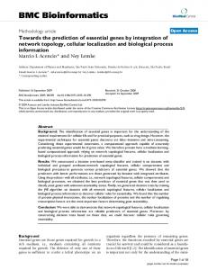
Fig. 1 Gene expression (reported significant genes detected only by knnAUC) between kidney-cancer and normal groups

Li et al. BMC Bioinformatics

(2018) 19:448

The uniquely significant genes detected by knnAUC and the corresponding P-values of all methods are shown in Additional file 2. And genes reported in pubmed (indicating that there is an abstract in Pubmed concerning a relationship with kidney cancer and the gene) are shown in Additional file 2 and Fig. 1 (Scatterplot and probability density distribution). Similarly, the uniquely significant genes found by other methods are shown in Additional file 3 and the genes reported in pubmed are showed in Fig. 2, 3, 4, 5 and 6. From the unique set of genes detected by knnAUC (Additional file 2), four genes, APOE, DSC2, SEC63 and SYCP1 were reported to be relevant to renal cancer (Fig. 1). A functional region of APOE could increase renal cell carcinoma susceptibility in a two stage case-control study [28]. DSC2 is associated with development and progression of renal cell carcinoma (RCC) [29]. SEC63 is associated with polycystic kidney disease [30, 31]. And copy-number gain of SYCP1 in human clear cell renal cell carcinoma predicts poor survival [32]. Although the distributions of these genes have

Page 6 of 12

almost the same mean value and different curvature of the density distribution function, the AUC values of these genes’ prediction models are significantly higher than 0.5, which could be detected by knnAUC method. UGT1A9 (identified in Additional file 3, Fig. 2) were the unique gene (also reported in pubmed database) detected by CANOVA. A significant decrease glucuronidation capacity of neoplastic kidneys versus normal kidneys was related with reduced UGT1A9 and UGT2B7 mRNA and protein expression [33]. Two unique genes (also reported in pubmed database) were detected by distance correlation. They were CITED1 and FIGF (identified in Additional file 3, Fig. 3). CITED1 confers stemness to Wilms tumor and enhances tumorigenic responses [34]. FIGF was related with the development of kidney in murine [35]. The two unique genes detected by logistic regression were GRPR and PRODH (identified in Additional file 3, Fig. 4). As a receptor for gastrin-releasing peptide (GRP), GRPR promotes renal cell carcinoma by activating ERK1/2 pathway together with GRP [36]. PRODH is among a few genes

Fig. 2 Gene expression (reported significant genes detected only by CANOVA) between kidney-cancer and normal groups

Li et al. BMC Bioinformatics

(2018) 19:448

Fig. 3 Gene expression (reported significant genes detected only by distance) between kidney-cancer and normal groups

Fig. 4 Gene expression (reported significant genes detected only by logistic regression) between kidney-cancer and normal groups

Page 7 of 12

Li et al. BMC Bioinformatics

(2018) 19:448

Page 8 of 12

Fig. 5 Gene expression (reported significant genes detected only by MIC) between kidney-cancer and normal groups

induced rapidly and robustly by P53, the tumor suppressor [37, 38]. MIC detected one gene, S100A1 (identified in Additional file 3, Fig. 5). HNF1β and S100A1 are useful biomarker for distinguishing renal oncocytoma and chromophobe renal cell carcinoma [39]. Six unique genes (also reported in pubmed database) were detected by KS test. They were SIX2, EPO, ASPSCR1, FOXD1, EGR1 and LPO. SIX2 is activated in renal neoplasms and influences cellular proliferation and migration [40]. EPO is related to the development of renal cell carcinoma [41]. A total of five TFE3 gene fusions (PRCC-TFE3, ASPSCR1-TFE3, SFPQ-TFE3, NONO-TFE3 and CLTC-TFE3) have been identified in RCC tumors and characterized at the mRNA transcript level [42]. FOXD1 is an upstream regulator of the renin-angiotensin system during metanephric kidney development [43]. MAML1 acts cooperatively with EGR1 to activate EGR1-regulated promoters, which could also have implications for the development of renal cell carcinoma [44]. Compared to normal renal cortex, the LPO induction period was markedly increased in renal-cell carcinoma [45, 46].

Discussion and conclusions Recently, correlations among inflammation grades, gene expressions and clinical parameters (serum alanine amino transaminase, aspartate amino transaminase and HBVDNA) were analyzed based on a large-scale CHB (chronic hepatitis B) samples [17]. The gene expressions with three clinical parameters in 122 CHB samples was analyzed by improved regression model and principal component analysis [17]. We found that significant genes, such as DLX3, ALPK1, YBX1, DCTN4, NKAPL, ZNF75A, SPP2 and AGAP3 (shown in Table 2), related to clinical parameters have a significant correlation with inflammation grades. Among all the benchmarked methods, knnAUC detected four unique genes related to renal cancer in pubmed database. Two of these genes were reported to be associated with renal cell carcinoma (RCC). MACC1 and DSC2 are related to the prognosis of RCC [29, 47]. The up-regulation of PDE2A methylation level was reported to promote the development of renal kidney papillary cell carcinoma (KIRP) [48]. Finally, NMD3 has been associated with the suppression of Wilms’ tumor through gene-specific interaction with GRC5 [49].

Li et al. BMC Bioinformatics

(2018) 19:448

Page 9 of 12

Fig. 6 Gene expression (reported significant genes detected only by KS) between kidney-cancer and normal groups

The non-linear dependence in our study is on the raw scale between one continuous variable and one binary variable, and other transformations will also be considered in our future studies. Theoretically, any machine learning algorithm could be the kernel function of the AUC based independence test we’ve developed. We also tested the performance of random forest [50], support vector machines [51] and generalized boosted models [52] as the kernels, however, they are not as powerful as knnAUC. And k-NN is a classic non-parametric method in machine learning area. But k-NN fails in case of the curse of dimensionality [53]. The curse of dimensionality in the k-NN basically means that Euclidean distance is not helpful in the presence of high dimensions because all vectors are almost equidistant to the search query vector. To avoid overfitting, we only resampled the dataset once which is equivalent to “an independent randomized trial” in statistics. Another advantage of knnAUC is that, it is robust with its two parameters,

ratio (the training sample size ratio) and kmax (automatically find the best parameter for knn between 1 and kmax). The knn algorithm was realized by RWeka package [14]. The ratio and kmax don’t significant influence the knnAUC performance. However, they may influence the computing time. For computational efficiency, using default parameters (ratio = 0.46 and k = 100), knnAUC could have competitive results. knnAUC is rather stable when the sample size is large enough (like > 100, we used knnAUC to recalculate Table 1 for 100 times in Additional file 4). And we may sometimes change the parameter ratio when the sample is extreme unbalanced (Additional file 5). For example, when you have too much cases such as 80~ 90% of total samples, you may want to set ratio = 0.1 or 0.2 to get more training samples in knnAUC method. When the average proportion of cases (Y = 1) was above 0.87, we found that the best parameter ratio was almost always 0.1 in Additional file 5. On the

Li et al. BMC Bioinformatics

(2018) 19:448

other hand, when the sample is not so extreme unbalanced (60~ 70% samples are cases), knnAUC performed well with the default parameters (ratio = 0.46) in Additional file 5. In practice, we can use grid search to tune the two parameters to improve power. For example, the parameter ratio can be tuned from 0.1 to 0.9 by 0.1, and the parameter kmax can be tuned from 2 to sample size by 1 to maximize detection power. Several methods were proposed to identification of genes related to a certain kind of cancer [54, 55]. In this article, the gene expression datasets are used to explain the purpose of our knnAUC method: detecting non-linear dependence biological signals between one continuous variable X and one binary variable Y. Furthermore, we could quantize the forecast skills of X by AUC and test whether it is significantly above 0.5. That is to say, knnAUC could be used to detect non-linear biological signals, which may be validated by further mechanism experiments. To sum, we developed an open-source R Package to detect dependence between one continuous variable and one binary variable especially under complex non-linear situations. We concluded that knnAUC (https://sourceforge.net/projects/knnauc/) is an efficient R package to test non-linear dependence between one continuous variable and one binary dependent variable especially in computational biology area.

Availability and requirements Project name: knnAUC. Project home page: https://sourceforge.net/projects/ knnauc/ Operating system(s): Windows or Linux. Programming language: R. License: GPL-2. Any restrictions to use by non-academics: licence needed.

Page 10 of 12

information-based nonparametric exploration; PCA: Principal component analysis; RCC: Renal cell carcinoma; RKHSs: Reproducing kernel Hilbert spaces; ROC: Response operating characteristic Acknowledgments The computations involved in this study were supported by the Fudan University High-End Computing Center. The views expressed in this presentation do not necessarily represent the views of the NIMH, NIH, HHS or the United States Government. This work was also supported by the Postdoctoral Science Foundation of China (2018M640333). Funding This research was supported by the National Basic Research Program (2014CB541801), National Science Foundation of China (31521003, 31330038), Ministry of Science and Technology (2015FY111700), Shanghai Municipal Science and Technology Major Project (2017SHZDZX01), and the 111 Project (B13016) from Ministry of Education (MOE). Availability of data and materials The kidney RNA-seq dataset were downloaded from the TCGA datasets (level 3 in TCGA datasets, http://cancergenome.nih.gov/). The chronic hepatitis B data discussed in this publication have been deposited in NCBI’s Gene Expression Omnibus and are accessible through accession number GSE83148 (https://www.ncbi.nlm.nih.gov/). Authors’ contributions YL, YW and LJ conceived the idea, proposed the knnAUC method. YL, XYL and YYS contributed to writing of the paper. YL, YW, YYS and LJ contributed to the theoretical analysis. YL also contributed to the development of knnAUC software using R. YL used R to generate tables and figures for all simulated and real datasets. YYM, WZ, ZHY, JL and JCW supported the chronic hepatitis B dataset. MMX helped support the kidney RNA-seq dataset. YL, XYL, MH, JCW and YYS contributed to scientific discussion and manuscript writing. LJ contributed to final revision of the paper. All authors read and approved the final manuscript. Ethics approval and consent to participate The kidney RNA-seq dataset are available in TCGA (http://cancergenome.nih.gov/), and the chronic hepatitis B dataset are accessible in NCBI (https:// www.ncbi.nlm.nih.gov/). Therefore, the patient consent was not required. Consent for publication Not applicable. Competing interests The authors declare that they have no competing interests.

Publisher’s Note Additional files Additional file 1: The power comparison of simulation study across different variance levels. (XLSX 14 kb) Additional file 2: The significant (associated with kidney cancer) genes only detected by knnAUC. (XLSX 16 kb) Additional file 3: The significant (associated with kidney cancer) genes only detected by other methods. (XLSX 106 kb) Additional file 4: The recalculated (100 times) simulation power of knnAUC with default parameters in nine simple functions. (XLSX 37 kb) Additional file 5: The simulation power of knnAUC with different ratios in nine simple functions. (XLSX 22 kb) Abbreviations AUC: Area under curve; CHB: Chronic hepatitis; GRP: Gastrin-releasing peptide; HBV: Chronic hepatitis B virus; KIRP: Renal kidney papillary cell carcinoma; knnAUC: K-nearest neighbors AUC test); MCM3: Minichromosome maintenance 3; MIC: Maximal information coefficient; MINE: Maximal

Springer Nature remains neutral with regard to jurisdictional claims in published maps and institutional affiliations. Author details 1 Ministry of Education Key Laboratory of Contemporary Anthropology, Department of Anthropology and Human Genetics, School of Life Sciences, Fudan University, Shanghai, China. 2Six Industrial Research Institute, Fudan University, Shanghai, China. 3State Key Laboratory of Genetic Engineering, Collaborative Innovation Center for Genetics and Development, School of Life Sciences, Fudan University, Shanghai, China. 4Department of Computational Medicine & Bioinformatics, University of Michigan, Ann Arbor, MI, USA. 5Shanghai Public Health Clinical Center, Fudan University, Shanghai, China. 6Key Laboratory of Medical Molecular Virology of MOE/MOH, Shanghai Medical School, Fudan University, Shanghai, China. 7Department of Digestive Diseases of Huashan Hospital, Collaborative Innovation Center for Genetics and Development, Fudan University, Shanghai, China. 8Human Genetics Center, School of Public Health, University of Texas Houston Health Sciences Center, Houston, TX, USA. 9Human Phenome Institute, Fudan University, Shanghai, China. 10Unit on Statistical Genomics, Division of Intramural Division Programs, National Institute of Mental Health, National Institutes of Health, Bethesda, MD, USA.

Li et al. BMC Bioinformatics

(2018) 19:448

Received: 12 February 2018 Accepted: 10 October 2018

References 1. Croxton FE, Cowden DJ: Applied general statistics. 1939. 2. Daniel WW. Applied Nonparametric Statistics. The Duxbury Advanced Series in Statistics and Decision Sciences; 1990. 3. Reshef DN, Reshef YA, Finucane HK, Grossman SR, McVean G, Turnbaugh PJ, Lander ES, Mitzenmacher M, Sabeti PC. Detecting novel associations in large data sets. Science. 2011;334(6062):1518–24. 4. Freedman DA: Statistical models: theory and practice: cambridge university press; 2009. 5. Walker SH, Duncan DB. Estimation of the probability of an event as a function of several independent variables. Biometrika. 1967;54(1–2):167–79. 6. Cox DR. The regression analysis of binary sequences. J R Stat Soc Ser B Methodol. 1958:215–42. 7. Székely GJ, Rizzo ML, Bakirov NK. Measuring and testing dependence by correlation of distances. Ann Stat. 2007;35(6):2769–94. 8. Kosorok MR. On Brownian distance covariance and high dimensional data. Ann Appl Stat. 2009;3(4):1266. 9. Marsaglia G, Tsang WW, Wang J. Evaluating Kolmogorov’s distribution. J Stat Softw. 2003;8(18):1–4. 10. Gretton A, Bousquet O, Smola A, Schölkopf B. Measuring statistical dependence with Hilbert-Schmidt norms. In International conference on algorithmic learning theory. Berlin: Springer. 2005. p. 63–77. 11. Heller R, Heller Y, Gorfine M. A consistent multivariate test of association based on ranks of distances. Biometrika. 2012;100(2):503–10. 12. Wang Y, Li Y, Cao H, Xiong M, Shugart YY, Jin L. Efficient test for nonlinear dependence of two continuous variables. BMC bioinformatics. 2015;16(1): 260. 13. Altman NS. An introduction to kernel and nearest-neighbor nonparametric regression. Am Stat. 1992;46(3):175–85. 14. Hall M, Frank E, Holmes G, Pfahringer B, Reutemann P, Witten IH. The WEKA data mining software: an update. ACM SIGKDD Explorations Newsletter. 2009;11(1):10–8. 15. Burke DS, Brundage JF, Redfield RR, Damato JJ, Schable CA, Putman P, Visintine R, Kim HI. Measurement of the false positive rate in a screening program for human immunodeficiency virus infections. N Engl J Med. 1988; 319(15):961–4. 16. Cohen J. Statistical power analysis for the behavioral sciences. 1988. Hillsdale: L. Lawrence Earlbaum Associates; 1988. p. 2. 17. Zhou W, Ma Y, Zhang J, Hu J, Zhang M, Wang Y, Li Y, Wu L, Pan Y, Zhang Y. Predictive model for inflammation grades of chronic hepatitis B: large-scale analysis of clinical parameters and gene expressions. Liver Int. 2017;37(11): 1632–41. 18. Jiang J, Lin N, Guo S, Chen J, Xiong M. Methods for joint imaging and RNAseq data analysis. arXiv preprint arXiv:1409.3899. 2014. 19. Network CGAR. Comprehensive molecular characterization of clear cell renal cell carcinoma. Nature. 2013;499(7456):43. 20. Mason SJ, Graham NE. Areas beneath the relative operating characteristics (ROC) and relative operating levels (ROL) curves: statistical significance and interpretation. Q J R Meteorol Soc. 2002;128(584):2145–66. 21. Hanley JA, McNeil BJ. The meaning and use of the area under a receiver operating characteristic (ROC) curve. Radiology. 1982;143(1):29–36. 22. Reshef D, Reshef Y, Mitzenmacher M, Sabeti P. Equitability analysis of the maximal information coefficient, with comparisons. arXiv preprint arXiv:1301. 6314. 2013. 23. Székely GJ, Rizzo ML. Energy statistics: a class of statistics based on distances. J Stat Plann Inference. 2013;143(8):1249–72. 24. Harrell FE, Dupont C. Hmisc: harrell miscellaneous. R Package Version. 2018; 4(1):1–401. 25. Albanese D, Filosi M, Visintainer R, Riccadonna S, Jurman G, Furlanello C. Minerva and minepy: a C engine for the MINE suite and its R, Python and MATLAB wrappers. Bioinformatics. 2012;29(3):407–8. 26. Tripodi G, Larsson SB, Norkrans G, Lindh M. Smaller reduction of hepatitis B virus DNA in liver tissue than in serum in patients losing HBeAg. J Med Virol. 2017;89(11):1937–43. 27. Salam O, Baiuomy AR, El-Shenawy SM, Hassan NS. Effect of pentoxifylline on hepatic injury caused in the rat by the administration of carbon tetrachloride or acetaminophen. Pharmacol Rep. 2005;57(5):596–603.

Page 11 of 12

28. Moore LE, Brennan P, Karami S, Menashe I, Berndt SI, Dong LM, Meisner A, Yeager M, Chanock S, Colt J, et al. Apolipoprotein E/C1 locus variants modify renal cell carcinoma risk. Cancer Res. 2009;69(20):8001–8. 29. Grigo K, Wirsing A, Lucas B, Klein-Hitpass L, Ryffel GU. HNF4α orchestrates a set of 14 genes to down-regulate cell proliferation in kidney cells. Biol Chem. 2008;389(2):179–87. 30. Bergmann C, Weiskirchen R. It’s not all in the cilium, but on the road to it: genetic interaction network in polycystic kidney and liver diseases and how trafficking and quality control matter. J Hepatol. 2012;56(5):1201–3. 31. Fedeles SV, Tian X, Gallagher AR, Mitobe M, Nishio S, Lee SH, Cai Y, Geng L, Crews CM, Somlo S. A genetic interaction network of five genes for human polycystic kidney and liver diseases defines polycystin-1 as the central determinant of cyst formation. Nat Genet. 2011;43(7):639–47. 32. Harlander S, Schonenberger D, Toussaint NC, Prummer M, Catalano A, Brandt L, Moch H, Wild PJ, Frew IJ. Combined mutation in Vhl, Trp53 and Rb1 causes clear cell renal cell carcinoma in mice. Nat Med. 2017;23(7):869–77. 33. Margaillan G, Rouleau M, Fallon JK, Caron P, Villeneuve L, Turcotte V, Smith PC, Joy MS, Guillemette C. Quantitative profiling of human renal UDPglucuronosyltransferases and glucuronidation activity: a comparison of normal and tumoral kidney tissues. Drug Metab Dispos. 2015;43(4):611–9. 34. Murphy AJ, Pierce J, de Caestecker C, Ayers GD, Zhao A, Krebs JR, Saito-Diaz VK, Lee E, Perantoni AO, de Caestecker MP, et al. CITED1 confers stemness to Wilms tumor and enhances tumorigenic responses when enriched in the nucleus. Oncotarget. 2014;5(2):386–402. 35. Avantaggiato V, Orlandini M, Acampora D, Oliviero S, Simeone A. Embryonic expression pattern of the murine figf gene, a growth factor belonging to platelet-derived growth factor/vascular endothelial growth factor family. Mech Dev. 1998;73(2):221–4. 36. Ischia J, Patel O, Sethi K, Nordlund MS, Bolton D, Shulkes A, Baldwin GS. Identification of binding sites for C-terminal pro-gastrin-releasing peptide (GRP)-derived peptides in renal cell carcinoma: a potential target for future therapy. BJU Int. 2015;115(5):829–38. 37. Phang JM. Proline metabolism in cell regulation and Cancer biology: recent advances and hypotheses. Antioxid Redox Signal. 2017;0(0):1–15. 38. Phang JM, Liu W. Proline metabolism and cancer. Front Biosci. 2012;17:1835–45. 39. Conner JR, Hirsch MS, Jo VY. HNF1beta and S100A1 are useful biomarkers for distinguishing renal oncocytoma and chromophobe renal cell carcinoma in FNA and core needle biopsies. Cancer Cytopathol. 2015;123(5):298–305. 40. Senanayake U, Koller K, Pichler M, Leuschner I, Strohmaier H, Hadler U, Das S, Hoefler G, Guertl B. The pluripotent renal stem cell regulator SIX2 is activated in renal neoplasms and influences cellular proliferation and migration. Hum Pathol. 2013;44(3):336–45. 41. Morais C, Johnson DW, Vesey DA, Gobe GC. Functional significance of erythropoietin in renal cell carcinoma. BMC Cancer. 2013;13:14. 42. Kauffman EC, Ricketts CJ, Rais-Bahrami S, Yang Y, Merino MJ, Bottaro DP, Srinivasan R, Linehan WM. Molecular genetics and cellular features of TFE3 and TFEB fusion kidney cancers. Nat Rev Urol. 2014;11(8):465–75. 43. Song R, Lopez M, Yosypiv IV. Foxd1 is an upstream regulator of the reninangiotensin system during metanephric kidney development. Pediatr Res. 2017;82(5):855–62. 44. Hansson ML, Behmer S, Ceder R, Mohammadi S, Preta G, Grafstrom RC, Fadeel B, Wallberg AE. MAML1 acts cooperatively with EGR1 to activate EGR1-regulated promoters: implications for nephrogenesis and the development of renal cancer. PLoS One. 2012;7(9):e46001. 45. Nikiforova NV, Khodyreva LA, Kirpatovskii VI, Chumakov AM. Lipid peroxidation in malignant tumors of human kidneys. Bull Exp Biol Med. 2001;132(5):1096–9. 46. Sverko A, Sobocanec S, Kusic B, Macak-Safranko Z, Saric A, Lenicek T, Kraus O, Andrisic L, Korolija M, Balog T, et al. Superoxide dismutase and cytochrome P450 isoenzymes might be associated with higher risk of renal cell carcinoma in male patients. Int Immunopharmacol. 2011;11(6): 639–45. 47. Betsunoh H, Fukuda T, Anzai N, Nishihara D, Mizuno T, Yuki H, Masuda A, Yamaguchi Y, Abe H, Yashi M. Increased expression of system large amino acid transporter (LAT)-1 mRNA is associated with invasive potential and unfavorable prognosis of human clear cell renal cell carcinoma. BMC Cancer. 2013;13(1):509. 48. Doecke JD, Wang Y, Baggerly K. Co-localized genomic regulation of miRNA and mRNA via DNA methylation affects survival in multiple tumor types. Cancer Genet. 2016;209(10):463–73.

Li et al. BMC Bioinformatics

(2018) 19:448

49. Karl T, Önder K, Kodzius R, Pichová A, Wimmer H, Thür A, Hundsberger H, Löffler M, Klade T, Beyer A. GRC5 and NMD3 function in translational control of gene expression and interact genetically. Curr Genet. 1999;34(6):419–29. 50. Breiman L. Random Forests. Mach Learn. 2001;45(1):5–32. 51. Cortes C, Vapnik V. Support-vector networks. Mach Learn. 1995;20(3):273–97. 52. G R: Generalized Boosted Models: A guide to the gbm package. In.; 2007. 53. Beyer K, Goldstein J, Ramakrishnan R, Shaft U. When Is “Nearest Neighbor” Meaningful? Berlin: Springer Berlin Heidelberg; 1999. p. 217–35. 54. Lemos C, Soutinho G, Braga AC. Arrow Plot for Selecting Genes in a Microarray Experiment: An Explorative Study. Cham: Springer International Publishing; 2017. p. 574–85. 55. Silva-Fortes C, Amaral Turkman MA, Sousa L. Arrow plot: a new graphical tool for selecting up and down regulated genes and genes differentially expressed on sample subgroups. BMC Bioinformatics. 2012;13:147.

Page 12 of 12