L2RM: Low-rank Linear Regression Models for High

L2RM: Low-rank Linear Regression Models for High-dimensional Matrix Responses Dehan Kong Department of Statistical Sciences, University of Toronto Baiguo An School of Statistics, Capital University of Economics and Business Jingwen Zhang and Hongtu Zhu Department of Biostatistics, University of North Carolina at Chapel Hill November 2018

Abstract The aim of this paper is to develop a low-rank linear regression model (L2RM) to correlate a high-dimensional response matrix with a high dimensional vector of covariates when coefficient matrices have low-rank structures. We propose a fast and efficient screening procedure based on the spectral norm of each coefficient matrix in order to deal with the case when the number of covariates is extremely large. We develop an efficient estimation procedure based on the trace norm regularization, which explicitly imposes the low rank structure of coefficient matrices. When both the dimension of response matrix and that of covariate vector diverge at the exponential order of the sample size, we investigate the sure independence screening property under some mild conditions. We also systematically investigate some theoretical properties of our estimation procedure including estimation consistency, rank consistency and non-asymptotic error bound under

some mild conditions. We further establish a theoretical guarantee for the overall solution of our two-step screening and estimation procedure. We examine the finite-sample performance of our screening and estimation methods using simulations and a large-scale imaging genetic dataset collected by the Philadelphia Neurodevelopmental Cohort (PNC) study. Keywords: Imaging Genetics, Low Rank, Matrix Linear Regression, Spectral norm, Trace norm.

1

Introduction

Multivariate regression modeling with a matrix response Y ∈ Rp×q and a multivariate covariate x ∈ Rs is an important statistical tool in modern high-dimensional inference, with wide applications in various large-scale applications, such as imaging genetic studies. Specifically, in imaging genetics, matrix responses (Y) as phenotypic variables often represent the weighted (or binary) adjacency matrix of a finite graph for characterizing structural (or functional) connectivity pattern, whereas covariates (x) include genetic markers (e.g., single nucleotide polymorphisms (SNPs)), age, and gender, among others. The joint analysis of imaging and genetic data may ultimately lead to discoveries of genes for many neuropsychiatric and neurological disorders, such as schizophrenia (Scharinger et al., 2010; Peper et al., 2007; Chiang et al., 2011; Thompson et al., 2013; Medlan et al., 2014). This motivates us to systematically investigate a statistical model with a multivariate response Y and a multivariate covariate x. Let {(xi , Yi ) : 1 ≤ i ≤ n} denote independent and identically distributed (i.i.d.) observations, where xi = (xi1 , . . . , xis )T is a s × 1 vector of scalar covariates (e.g., clinical variables and genetic variants) and Yi is a p×q response matrix. Without loss of generality, we assume that xil has mean 0 and variance 1 for every 1 ≤ l ≤ s, and Yi has mean 0. Throughout the paper, we consider a L2RM, which is given by Yi =

s X

xil ∗ Bl + Ei ,

(1)

l=1

where Bl is a p × q coefficient matrix characterizing the effect of the lth covariate on Yi and 2

Ei is a p × q matrix of random errors with mean 0. The symbol “ ∗ ” denotes the scalar multiplication. Model (1) differs significantly from the existing matrix regression, which was developed for matrix covariates and univariate responses (Leng and Tang, 2012; Zhao and Leng, 2014; Zhou and Li, 2014). Our goal is to discover a small set of important covariates from x that strongly influence Y. We focus on the most challenging setting that both the dimension of Y (or pq) and that of x (or s) can diverge with the sample size. Such a setting is general enough to cover highdimensional univariate and multivariate linear regression models in the literature (Negahban et al., 2012; Fan and Lv, 2010; Buhlmann and van de Geer, 2011; Tibshirani, 1997; Yuan et al., 2007; Candes and Tao, 2007; Breiman and Friedman, 1997; Cook et al., 2013; Park et al., 2017). In the literature, there are two major categories of statistical methods for jointly analyzing high-dimensional matrix Y and high-dimensional vector x. The first category is a set of mass univariate methods. Specifically, it fits a marginal linear regression to correlate each element of Yi with each element of xi , leading to a total of pqs massive univariate analyses and an expanded search space with pqs elements. It is also called voxel-wise genome-wide association analysis (VGAWS) in the imaging genetics literature (Hibar et al., 2011; Shen et al., 2010; Huang et al., 2015; Zhang et al., 2014; Medland et al., 2014; Zhang et al., 2014; Thompson et al., 2014; Liu and Calhoun, 2014). For instance, Stein et al. (2010) used 300 high performance CPU nodes to run approximately 27 hours to carry out a VGWAS analysis on an imaging genetic dataset with only 448,293 SNPs and 31,622 imaging measures for 740 subjects. Such computational challenges are becoming more severe as the field is rapidly advancing to the most challenging setting with large pq and s. More seriously, for model (1), the massive univariate method can miss some important components of x that strongly influence Y due to the interaction among x. The second category is to fit a model accommodating all (or part of) covariates and responses (Vounou et al., 2010, 2012; Zhu et al., 2014; Wang et al., 2012a,b; Peng et al., 2010). These methods use regularization methods, such as Lasso or group Lasso, to select a set of covariate-response pairs. However, when the product pqs is extremely large, it is very difficult to allocate computer memory for such an array of size pqs in order to accommodate all coefficient matrices Bl s, rendering all these regularization methods being 3

intractable. Therefore, almost all existing methods in this category have to use some dimension reduction techniques (e.g., screening methods) to reduce both the number of responses and that of covariates. Subsequently, these methods fit a multivariate linear regression model with the selected elements of Y as new responses and those of x as new covariates. However, this approach can be unsatisfactory, since it does not incorporate the matrix structural information. The aim of this paper is to develop a low-rank linear regression model (L2RM) as a novel extension of both VGAWS and regularization methods. Specifically, instead of repeatedly fitting a univariate model to each covariate-response pair, we consider all elements in Yi as a high-dimensional matrix response and focus on the coefficient matrix of each covariate, which is approximately low-rank (Cand`es and Recht, 2009). There is a literature on the development of matrix variate regression (Ding and Cook, 2014; Fosdick and Hoff, 2015; Zhou and Li, 2014), but these papers focus on the case when covariates have a matrix structure. In contrast, there is a large literature on the development of various function-on-scalar regression models that emphasize the inherent functional structure of responses. See Chapter 13 of Ramsay and Silverman (2005) for a comprehensive review on this topic. Variable selection methods have been developed for some function-on-scalar regression models (Wang et al., 2007; Chen et al., 2016), but these methods focus on one-dimensional functional response rather than two-dimensional matrix response. Recently, there has been some literature considering matrix or tensor responses regression (Ding and Cook, 2018; Li and Zhang, 2017; Raskutti and Yuan, 2018; Rabusseau and Kadri, 2016), but they only consider the case when the dimension of the covariates is fixed or slowly diverging with the sample size. In this paper, we aim at efficiently correlating matrix responses with a high dimensional vector of covariates. Four major methodological contributions of this paper are as follows. • We introduce a low-rank linear regression model to fit high-dimensional matrix responses with a high dimensional vector of covariates, while explicitly accounting for the low-rank structure of coefficient matrices. • We introduce a novel rank-one screening procedure based on the spectral norm of the estimated coefficient matrix to eliminate most “noisy” scalar covariates and show that 4

our screening procedure enjoys the sure independence screening property (Fan and Lv, 2008) with vanishing false selection rate. The use of such spectral norm is critical for dealing with a large number of noisy covariates. • When the number of covariates is relatively small, we propose a low rank estimation procedure based on trace norm regularization, which explicitly characterizes the lowrank structure of coefficient matrices. An efficient algorithm for solving the optimization problem is developed. We systematically investigate some theoretical properties of our estimation procedure, including estimation and rank consistency when both p and q are fixed and an non-asymptotic error bound when both p and q are allowed to diverge. • We investigate how incorrectly screening results can affect the low-rank regression model estimation both numerically and theoretically. We establish a theoretical guarantee for the overall solution, while accounting for the randomness of the first-step screening procedure. The rest of this paper is organized as follows. In Section 2, we introduce a rank-one screening procedure to deal with a high dimensional vector of covariates and describe our estimation procedure when the number of covariates is relatively small. Section 3 investigates the theoretical properties of our method. Simulations are conducted in Section 4 to evaluate the finite-sample performance of the proposed two-step screening and estimation procedure. Section 5 illustrates an application of L2RM in the joint analysis of imaging and genetic data from the Philadelphia Neurodevelopmental Cohort (PNC) study discussed above. We finally conclude with some discussions in Section 6.

2

Methodology

Throughout the paper, we focus on addressing three fundamental issues for L2RM as follows: • (I) The first one is to eliminate most ‘noisy’ covariates xil when the number of candidate covariates and that of response matrix are much larger than n, that is min(s, pq) >> n.

5

• (II) The second one is to estimate the coefficient matrix Bl when Bl does have a low-rank structure. • (III) The third one is to investigate some theoretical properties of the screening and estimation methods.

2.1

Rank-one Screening Method

We consider the case that both pq and s diverge at an exponential order of n, and we also denote s by sn . To address (I), it is common to assume that most scalar covariates have no effects on the matrix responses, that is, Bl0 = 0 for most 1 ≤ l ≤ sn , where Bl0 is the true value for Bl . In this case, we define the true model and its size as M = {1 ≤ l ≤ sn : Bl0 6= 0} and s0 = |M| < n.

(2)

Our aim is to estimate the set M and coefficient matrices Bl . Simultaneously estimating M and Bl is difficult since it is computationally infeasible to fit a model when both sn and pq are large. For example, in the PNC data, we have pq = 692 = 4, 761 and sn ≈ 5 × 106 . Therefore, it may be imperative to employ a screening technique to reduce the model size. However, developing a screening technique for model (1) can be more challenging than many existing screening methods, which focus on univariate responses (Fan and Lv, 2008; Fan and Song, 2010) . Similar to Fan and Lv (2008) and Fan and Song (2010), it is assumed that all covariates have been standardized so that E(xil ) = 0 and E(x2il ) = 1 for l = 1, . . . , sn . We also assume that every element of Yi = (Yi,jk ) has been standardized, that is, 2 E(Yi,jk ) = 0 and E(Yi,jk ) = 1 for j = 1, . . . , p and k = 1, . . . , q.

We propose to screen covariates based on the estimated marginal ordinary least squares b M = n−1 Pn xil ∗ Yi for l = 1, . . . , sn . Although the interpreta(OLS) coefficient matrix B l i=1 tions and implications of the marginal models are biased from the joint model, the nonsparse 6

information about the joint model can be passed along to the marginal model under a mild condition. Hence it is suitable for the purpose of variable screening (Fan and Song, 2010). bM, Specifically, we calculate the spectral norm (operator norm or largest singular value) of B l b M kop , and define a submodel as denoted as kB l b M kop ≥ γn }, cγn = {1 ≤ l ≤ sn : kB M l

(3)

where γn is a prefixed threshold. b M kop is that it explicitly accounts for the low-rank structure The key advantage of using kB l of Bl0 s for most noisy covariates, while being robust to noise and more sensitive to various signal patterns (e.g., sparsely strong signals and low rank weak signals) in coefficient matrices. In our screening step, we use the marginal OLS estimates of the coefficient matrices, which can be regarded as the true coefficient matrices corrupted with some noise. One may directly b M based on the component-wise information of B bM, use some other summary statistics of B l l b M k1 (sum of the absolute value of all the elements), kB b M kF , or the global Waldsuch as kB l l type statistic used in Huang et al. (2015). It is well known that those summary statistics are sensitive to noise and suffer from the curse of dimensionality. This is further confirmed b M kop is more robust to in our simulation studies that our rank-one screening based on kB l b M kop noise and sensitive to small signal regions. Moreover, the other advantage of using kB l is that it is computationally efficient. In contrast, we may calculate some other regularized estimates (e.g., Lasso or fused Lasso) for screening, but it is computationally infeasible for L2RM when sn is much larger than the sample size. A difficult issue in (3) is how to properly select γn . As shown in Section 3.1, when γn is chosen properly, our screening procedure enjoys the sure independence property (Fan and Lv, 2008). However, it is difficult to precisely determine γn in practice since it involves in two unknown positive constant terms C1 and α as shown in Theorem 1, which cannot be easily determined for finite sample. We propose to use random decoupling to select γn , which is similar to that used in Barut et al. (2016). Let {x∗i , i = 1, . . . , n} be a random permutation of the original data {xi , i = 1, . . . , n}. We apply our screening procedure on the random decoupling data {x∗i , Yi }ni=1 . As the original association between xi and Yi is destroyed by random decoupling, when we perform screening using {x∗i , Yi }ni=1 , it mimics the null model, 7

i.e. the model when there is no association. We obtain the estimated marginal coefficient b M )∗ , which is a statistical estimate of zero matrix, and the corresponding operator matrix (B l b M )∗ kop , which is the the b M )∗ kop for all 1 ≤ l ≤ sn . Define νn = max1≤l≤sn k(B norm k(B l l minimum thresholding parameter that makes no false positives. Since νn depends on the realization of the permutation, we set the threshold value γn as the median of these threshold (k)

(k)

values {νn , 1 ≤ k ≤ K} from K different random permutations, where νn is the threshold value for the kth permutation. We set K = 10 in this paper.

2.2

Estimation Method

To address (II), we consider the estimation of B when the true coefficient matrices Bl0 s truly have a low-rank structure. The following refined estimation step can be applied after the screening step when the number of covariates is relatively small. For simplicity, we denote cγn by M. c Suppose M c = {l1 , . . . , l c }, where the set selected by the screening step M |M| c c 1 ≤ l1 < . . . < l|M| ] ∈ Rp×q|M| . c ≤ sn . Define B = [Bl , l ∈ M] = [Bl1 , . . . , Bl|M| c P Recently, the trace norm regularization kBl k∗ = k σk (Bl ) has been widely used to

recover the low-rank structure of Bl due to its computational efficiency, where σk (Bl ) is the kth singular value of Bl . For instance, the trace norm has been used for matrix completion (Cand`es and Recht, 2009), for matrix regression models with matrix covariates and univariate responses (Zhou and Li, 2014), and for multivariate linear regression with vector responses and scalar covariates (Yuan et al., 2007). Similarly, we propose to calculate the regularized least squares estimator of B by minimizing n

X X 1 X Q(B) = kYi − xil ∗ Bl k2F + λ kBl k∗ , 2n i=1 c l∈M

(4)

c l∈M

where k · kF is the Frobenius norm of a matrix and λ is a tuning parameter. The low rank structure can be regarded as a special spatial structure, since it is very similar to functional principal component analysis. We use the five-fold cross validation to select the tuning parameter λ. Ideally, we may choose different tuning parameters for different Bl , but it can dramatically increase computational complexity. We apply the Nesterov gradient method to solve problem (4) even though Q(B) is nonsmooth (Nesterov, 2004; Beck and Teboulle, 2009). The Nesterov gradient method utilizes 8

the first-order gradient of the objective function to obtain the next iterate based on the current search point. Unlike the standard gradient descent algorithm, the Nesterov gradient algorithm uses two previous iterates to generate the next search point by extrapolating, which can dramatically improve the convergence rate. Before we introduce the Nesterov gradiant algorithm, we first state a singular value thresholding formula for the trace norm (Cai et al., 2010). Proposition 1. For a matrix A with {ak }1≤k≤r being its singular values, the solution to 1 min{ kB − Ak2F + λkBk∗ } B 2

(5)

shares the same singular vectors as A and its singular values are bk = (ak − λ)+ for k = 1, . . . , r. We present the Nesterov gradient algorithm for problem (4) as follows. Denote R(B) = P P P 2 (2n)−1 ni=1 kYi − l∈M c kBl k∗ . We also define c xil ∗ Bl kF and J(B) = λ l∈M g(B|S(t) , δ) = R(S(t) )+ < ∇R(S(t) ), B − S(t) > +(2δ)−1 kB − S(t) k2F + J(B) = (2δ)−1 kB − [S(t) − δ∇R(S(t) )]k2F + J(B) + c(t) , where ∇R(S(t) ) denotes the first-order gradient of R(S(t) ) with respect to S(t) , S(t) is an interpolation between B(t) and B(t−1) and will be defined below, c(t) denotes all terms that are irrelevant to B, and δ > 0 is a suitable step size. Given a previous search point S(t) , the next search point S(t+1) would be the minimizer of g(B|S(t) , δ). For the search point S(t) , it can be generated by linearly extrapolating two previous algorithmic iterates. A key advantage of using the Nestrov gradient method is that it has an explicit solution at each (t)

iteration. Specifically, let Bld , Sld , and ∇R(S(t) )ld be the (dq − q + 1)th to the dqth columns c matrices B, S(t) , and ∇R(S(t) ), respectively. Minimizing of the corresponding p × q|M| P c (2δ)−1 kB − [S(t) − δ∇R(S(t) )]k2F + λ l∈M c kBl k∗ is equivalent to solving |M| sub-problems, (t) c each of which minimizes (2δ)−1 kBld − [Sld − δ∇R(S(t) )ld ]k2F + λkBld k∗ for d = 1, . . . , |M|,

while each sub-problem can be exactly solved by using the singular value thresholding formula given in Proposition 1. c Define XM c = (xil )1≤i≤n,l∈M c is an n × |M| matrix and λmax (·) denotes the largest eigenvalue of a matrix. Our algorithm can be stated as follows: 9

T 1. Initialize B(0) = B(1) , α(0) = 0 and α(1) = 1, t = 1, and δ = n/λmax {(XM c ) XM c}.

2. Repeat (t)

S(t) = B(t) + ( αα(t)−1 )(B(t) − B(t−1) ); c for d = 1 : |M|, (t)

i. (Atemp )ld = Sld − δ∇R(S(t) )ld ; ii. compute singular value decomposition (SVD) (Atemp )ld = Uld diag(ald )VlTd ; iii. bld = ald − λδ ∗ 1; iv. (Btemp )ld = Uld diag(bld )VlTd ; end c sub-matrices and get the entire matrix Btemp ; Combine {(Btemp )ld , 1 ≤ d ≤ |M|} B(t+1) = Btemp ; p α(t+1) = {1 + 1 + (2α(t) )2 }/2; t = t + 1; 3. until objective function Q(B(t) ) converges. c matrices Atemp and Btemp , (Atemp )l and (Btemp )l denote the (dq − For the above p × q|M| d d q + 1)th to the (dq)th columns of the corresponding matrices, respectively. A sufficient condition for the convergence of {B(t) }t≥1 is that the step size δ should be smaller than or equal to 1/L(R), where L(R) is the smallest Lipschitz constant of the function R(B) (Beck and Teboulle, 2009; Facchinei and Pang, 2003). In our case, L(R) is T equal to n−1 λmax {(XM c ) XM c}.

Remarks: For model (1), it is assumed that xil has mean 0 and variance 1 for every 1 ≤ l ≤ s, and Yi has mean 0 throughout the paper. If these assumptions are not valid in practice, a simple solution is to carry out a standardization step including standardizing covariates and centering responses. We use this approach in simulations and real data analysis. An alternative approach is to introduce an intercept matrix term B0 in model (1). M Our screening procedure is invariant to such standardization step if we calculate Bl,jk , the

(j, k)−th element of Bl , as the sample correlation between xil and Yi,jk . In the Supplementary Material, we present a modified algorithm of our estimation procedure and evaluate the effects of the standardization step on estimating Bl by using simulations. According to our 10

experience, scaling covariates is necessary in order to ensure that all covariates are at the same scale, whereas centering covariates and responses is not critical.

3

Theoretical Properties

To address (III), we systematically investigate several key theoretical properties of the screening procedure and the regularized estimation procedure as well as a theoretical guarantee of our two-step estimator. First, we investigate the sure independence screening property of the rank-one screening procedure when s (also denoted by sn ) diverges at an exponential rate of the sample size. Second, we investigate the estimation and rank consistency of our regularized estimator when both p and q are fixed. Third, we derive the non-asymptotic error bound for our estimator when both p and q are diverging. Finally, we establish an overall theoretical guarantee for our two-step estimator. We state the following theorems, whose detailed proofs can be found in the Appendix B.

3.1

Sure Screening Property

The following assumptions are used to facilitate the technical details, even though they may not be the weakest conditions but help to simplify the proof. (A0) The covariates xi are i.i.d from a distribution with mean 0 and covariance matrix Σx . Define σl2 = (Σx )ll . The vectorized error matrices vec(Ei ) are i.i.d from a distribution with 0 and covariance matrix Σe , where vec(·) denotes the vectorization of a matrix. Moreover, xi and Ei = (Ei,jk ) are independent. (A1) There exist some constants C1 > 0, b > 0, and 0 < κ < 1/2 such that min kcov( l∈M

X

xil0 ∗ Bl0 0 , xil )kop ≥ C1 (pq)1/2 n−κ and max kBl0 k∞ < b, l∈M

l0 ∈M

P P where cov( l0 ∈M xil0 ∗Bl0 0 , xil ) is a p×q matrix with the (j, k)th element being cov( l0 ∈M xil0 ∗ Bl0 0,jk , xil ), and kBl0 k∞ = max1≤j≤p,1≤k≤q |Bl0,jk |. (A2) There exist positive constants C2 and C3 such that 2 max(E{exp(C2 x2il )}, E{exp(C2 Ei,jk )}) ≤ C3

11

for every 1 ≤ l ≤ sn , 1 ≤ j ≤ p and 1 ≤ k ≤ q. (A3) There exists a constant C4 > 0 such that log(sn ) = C4 nξ for ξ ∈ (0, 1 − 2κ). (A4) There exist constants C5 > 0 and τ > 0 such that λmax (Σx ) ≤ C5 nτ . (A5) We assume log(pq) = o(n1−2κ ).

Remarks: Assumptions (A0)-(A5) are used to establish the theory of our screening procedure when sn diverges to infinity. Assumption (A1) is analogous to Condition 3 in Fan and Lv (2008) and equation (4) in Fan and Song (2010), in which κ controls the rate of probability error in recovering the true sparse model. Assumption (A2) is analogous to Condition (D) in Fan and Song (2010) and Condition (E) in Fan et al. (2011). Assumption (A2) requires that xil and Ei,jk are sub-gaussian, which ensures the tail probability to be exponentially light. Assumption (A3) allows the dimension sn to diverge at an exponential rate of the sample size n, which is analogous to Condition 1 in Fan and Lv (2008). Assumption (A4) is analogous to Condition 4 in Fan and Lv (2008), which rules out the case of strong collinearity. Assumption (A5) allows the product of the row and column dimensions of the matrix pq to diverge at an exponential rate of the sample size n. The following theorems show the sure screening property of the screening procedure. We allow p and q to be either fixed or diverging with sample size n. Theorem 1. Under Assumptions (A0)-(A3) and (A5), let γn = αC1 (pq)1/2 n−κ with 0 < cγn ) → 1 as n → ∞. α < 1, then we have P (M ⊆ M Theorem 1 shows that if γn is chosen properly, then our rank-one screening procedure will not miss any significant variables with an overwhelming probability. Since the screening procedure automatically includes all the significant covariates for small values of γn , it is cγn when γn = αC1 (pq)1/2 n−κ holds. necessary to consider the size of M cγn | = O(n2κ+τ )) → 1 for γn = Theorem 2. Under Assumptions (A0)-(A5), we have P (|M αC1 (pq)1/2 n−κ with 0 < α < 1 as n → ∞. Theorem 2 indicates that the selected model size with the sure screening property is only at a polynomial order of n, even though the original model size is at an exponential order of n. Therefore, the false selection rate of our screening procedure vanishes as n → ∞. 12

3.2

Theory for Estimation Procedure

cγn by M c for notation simplicity. We first provide From this subsection, we will denote M some theoretical results for our estimation procedure. We assume that we can exactly select c = M, and s0 = |M| is fixed. The results are also all the important variables in M, i.e. M applicable if our original s is fixed, in which we only need to apply our estimation procedure. We need more notations before we introduce more assumptions. Suppose the rank of Bl0 T as the singular value decomposition of is rl . For every l = 1, . . . , sn , we denote Ul0 Θl0 Vl0

⊥ Bl0 and use U⊥ l0 and Vl0 to denote the orthogonal complements of Ul0 and Vl0 , respectively.

Define ΣM as the covariance matrix for xi,M , where xi,M = (xil )l∈M ∈ R|M| . We further ⊥ T define A = ΣM ⊗ Ipq×pq , Kl = Vl0 ⊗ U⊥ l0 and dl = −vec(Ul0 Vl0 ) for l ∈ M, where ⊗

denotes the Kronecker product. Let d = (dTl1 , . . . , dTl|M| )T and K = diag{Kl1 , . . . , Kl|M| }. We define Λl ∈ R(p−rl )×(q−rl ) for l ∈ M such that vec(Λ) = (vec(Λl1 )T , . . . , vec(Λl|M| )T )T = (KT A−1 K)−1 KT A−1 d. The Λl has some interesting interpretation. For instance, it can be shown that it is the Lagrange multiplier of an optimization problem. We include more interpretation of Λl in the Appendix C. We then state additional assumptions that are needed to establish the theory of our estimation procedure when both p and q are assumed to be fixed. The following assumptions (A6)-(A8) are needed. (A6) The ΣM is nonsingular. (A7) The maxl {rank(Bl0 ) : l ∈ M} < min(p, q) holds. (A8) For every l ∈ M, we assume kΛl kop < 1. Remarks:

Assumption (A6) is a regularity condition in the low dimensional context,

which rules out the scenario when one covariate is exactly a linear combination of other covariates. Assumption (A7) is used for rank consistency. Assumption (A8) can be regarded as the irrepresentable condition of Zhao and Yu (2006) in the rank consistency context. A similar condition can be found in Bach (2008). b l the regularized low rank estimator of Bl for l ∈ M. We have the following Define B consistent results when the tuning parameter converges in different rates when both p and q are fixed.

13

Theorem 3. (Estimation Consistency) Under Assumptions (A0) and (A6), we have b l − Bl0 ) = Op (1) for all l ∈ M; (i) if n1/2 λ → ∞ and λ → 0, then λ−1 (B b l − Bl0 ) = Op (1) for all l ∈ M. (ii) if n1/2 λ → ρ ∈ [0, ∞) and n → ∞, then n1/2 (B Theorem 3 reveals an interesting phase-transition phenomenon. When λ is relatively b l − Bl0 is of order n−1/2 , whereas as λ gets small or moderate, the convergence rate of B b l − Bl0 can be approximated as the order of λ. Although we large, the convergence rate of B b l as λ → 0, the next question is whether the rank of B bl have established the consistency of B is consistent under the same set of conditions. It turns out that such rank consistency only holds for relatively large λ, whose convergence rate is slower than n−1/2 . Theorem 4. (Rank Consistency) Under Assumptions (A0) and (A6)-(A8), if λ → 0 and b l ) = rank(Bl0 )) → 1 for all l ∈ M. n1/2 λ → ∞ hold, we have that P (rank(B Theorem 4 establishes the rank consistency of our regularized estimates. Theorems 3 and 4 reveal that both of the element consistency and the rank consistency hold only for λ → 0 and n1/2 λ → ∞. This phenomenon is similar to that for the Lasso estimator. Specifically, although the Lasso estimator can achieve model selection consistency, the convergence rate of the Lasso estimator cannot achieve the rate of n−1/2 when selection consistency is satisfied (Zou, 2006). We then consider the case when p and q are assumed to be diverging. The following assumptions (A9)-(A12) are needed.

(A9) There exist positive constants CL and CM such that 0 < CL ≤ λmin (ΣM ) ≤ λmax (ΣM ) ≤ CM < ∞. (A10) We assume that xi,M are i.i.d multivariate normal with mean 0 and covariance matrix ΣM . (A11) The vectorized error matrices vec(Ei ) are i.i.d N (0, Σe ), where λmax (Σe ) ≤ CU2 < ∞. (A12) We assume max(p, q) → ∞ and max(p, q) = o(n) as n → ∞. Remarks: Assumptions (A9)-(A12) are needed for our estimation procedure when both p and q are diverging with the sample size n. Assumption (A9) assumes the largest eigenvalue 14

of ΣM is bounded and the smallest eigenvalue of ΣM is greater than 0. Assumption (A10) assumes that the covariates xil s are gaussian. Assumption (A11) assumes that the largest eigenvalue of Σe is bounded. Assumption (A12) allows p and q to diverge slower than n, but it does allow that pq > n. We then show the following non-asymptotic bound for our estimation procedure when both p and q are diverging. Theorem 5. (Nonasymptotic bound when both p and q diverge) Under Assumptions 1/2

(A9)-(A12), when λ ≥ 4CU CM n−1/2 (p1/2 + q 1/2 ), there exist some positive constants c1 , c2 and c3 such that with probability at least 1 − c1 exp{−c2 (p + q)} − c3 exp(−n), we have b − B0 k2 ≤ C( kB F

X

rl )λ2 CL−2

l∈M

for some constant C > 0. Theorem 5 implies that when {rl , l ∈ M} and |M| are fixed and λ  n−1/2 (p1/2 + b would be consistent with probability going to 1. The convergence q 1/2 ), the estimator B rate of the estimator in Theorem 5 coincides with that in Corollary 5 of Negahban et al. (2009), where they studied the low-rank matrix learning problem using the trace norm regularization. Although considering different models, they also require the dimension of the matrix max(p, q) = o(n). It differs significantly from the L1 regularized problem, where the dimension of the matrix may diverge at the exponential order of the sample size. The result in this theorem can also be regarded as a special case of the result in Raskutti and Yuan (2018), where they derived non-asymptotic error bound in a class of tensor regression model with sparse or low-rank penalties.

3.3

Theory for Two-step Estimator

In this section, we give a unified theory for our two-step estimator. In particular, we derive the non-asymptotic bound for our final estimate. To begin with, we first introduce some c to denote M cγn , which is the set selected from the notations. For simplicity, we will use M c c c c c ∈ Rp×q|M| first step. Define BM = [Bl , l ∈ M] and the true value of BM as BM 0 = [Bl0 , l ∈ c c c bM b l , l ∈ M] c ∈ Rp×q|M| c ∈ Rp×q|M| M] . Define B = [B as the solution of the regularized trace

15

norm penalization problem given by n

X X 1 X min Q(B ) = min{ kYi − xil ∗ Bl k2F + λ kBl k∗ }. c c 2n i=1 BM BM c M

c l∈M

(6)

c l∈M

We need the following assumptions. (A13) Assume 2κ + τ < 1. Define ιL := minkδk0 ≤m,δ6=0 δ T (n−1

Pn

i=1

xi xTi )δ/kδk22 for any

m = O(n2κ+τ ) and δ ∈ Rs . We further assume ιL > 0. (A14) Assume max(p, q)/ log(n) → ∞ and max(p, q) = o(n1−2τ ) as n → ∞ with τ < 1/2. Theorem 6. (Nonasymptotic bound for two-step estimator) Under Assumptions (A0)-(A5), (A10), (A11), (A13), and (A14), when λ ≥ 4C5 nτ −1/2 (p1/2 + q 1/2 ), there exist some positive constants c1 , c2 , c3 , c4 , c5 such that with probability at least 1−c1 n2κ+τ exp{−c2 (p+ q)} − c3 n2κ+τ exp(−n) − c4 exp(−c5 n1−2κ ), we have b M − BM k2 ≤ C( kB 0 F c

c

X

rl )λ2 ι−2 L

l∈M

for some constant C > 0. Theorem 6 implies that when {rl : l ∈ M} and |M| are fixed and ιL is fixed, the estimator c bM B is consistent with probability going to 1 when λ  nτ −1/2 (p1/2 +q 1/2 ). Theorem 6 gives an

overall theoretical guarantee for our two-step estimator by considering the random selection procedure in the first step. A key fact that we use in the proof of Theorem 6 is that our first-step screening procedure enjoys the sure independence property. In this case, we only need to derive the non-asymptotic bound for the case when we exactly select or over-select the important variables as it holds with overwhelming probability.

4

Simulations

We conduct simulations to examine the finite sample performance of the proposed estimation and screening procedures. For the sake of space, we include additional simulation results in the Supplementary Material.

16

2

10

1.5

20

2

10

2

10

1.5

20

20

1

30

30 0.5 40 0

50

60

50 −0.5

60 20

30

40

50

60

60

(a)

20

30

40

50

−0.5 60

−1 10

0 50

−0.5

−1 10

0.5 40

0

−0.5

1

30

0.5 40

50

1.5

1

30

0

2

10

20

1

0.5 40

1.5

−1

60

10

(b)

20

30

40

50

60

−1 10

(c)

20

30

40

50

60

(d)

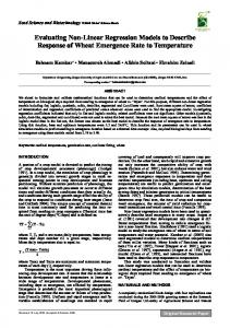
Figure 1: Simulation I setting: the four 64×64 true coefficient matrices for the first simulation setting: the cross shape for B10 in panel (a), the square shape for B20 in panel (b), the triangle shape of B30 in panel (c), and the butterfly shape for B40 in panel (d). The regression coefficient at each pixel is either 0 (blue) or 1 (yellow).

4.1

Regularized Low-rank Estimate

In the first simulation, we simulate 64 × 64 matrix responses according to model (1) with s = 4 covariates. We set the four true coefficient matrices to be a cross shape (B10 ), a square shape (B20 ), a triangle shape (B30 ), and a butterfly shape (B40 ). The images of Bl0 are shown in Figure 1, and each of them consists of a yellow region of interest (ROI) containing ones and a blue ROI containing zeros. We independently generate all scalar covariates xi from N (0, Σx ), where Σx = (σx,ll0 ) |l−l0 |

is a covariance matrix with an autoregressive structure such that σx,ll0 = ρ1

holds for

1 ≤ l, l0 ≤ s with ρ1 = 0.5. We independently generate vec(Ei ) from N (0, Σe ). Specifically, we set the variances of all elements in Ei to be σe2 and the correlation between Ei,jk and |j−j 0 |+|k−k0 |

Ei,j 0 k0 to be ρ2

for 1 ≤ j, k, j 0 , k 0 ≤ 64 with ρ2 = 0.5. We consider three different

sample sizes including n = 100, 200, and 500, and set σe2 to be 1 and 25. We use 100 replications to evaluate the finite sample performance of our regularized lowb l defined as kB b l − Bl0 k2 . To evaluate the estimation accuracy, we rank (RLR) estimates B F b l , denoted by MSE(B b l ), for all 1 ≤ l ≤ 4. We also compute the mean squared errors of B calculate the prediction errors (PE) by generating ntest = 500 independent test observations. We compare our method with OLS, Lasso, fused Lasso, and tensor envelope method (Li and Zhang, 2017). For fair comparison, we also use five-fold cross validation to select regularization parameters of Lasso and fused Lasso and the envelope dimension of the tensor envelope method. The results are shown in Table 1. We also plot the RLR, OLS, Lasso, 17

b l , 1 ≤ l ≤ 4} obtained from a randomly fused Lasso and tensor envelope estimates of {B selected data set with n = 500 and σe2 = 25 in Figure 2. Inspecting Figure 2 and Table 1 reveals the following findings. First, our method always outperforms OLS and envelope method. Second, when the images are of low rank (cross and square), our estimation method truly outperforms Lasso. Third, our method outperforms fused Lasso when either the sample size is small or the noise variance is large, whereas fused Lasso outperforms our method in other cases. Fourth, when the images are not of low rank (triangle and butterfly), fused Lasso performs best in most cases, whereas our method outperforms Lasso when either noise level is high or sample size is small. These findings are not surprising. First, in all settings, since all the true coefficient matrices are piecewise sparse, the fused Lasso method is expected to perform well. Second, Lasso works reasonably well since it still imposes sparse structure. Third, since our method is designed for low rank cases, it performs well for the low rank cross and square cases, whereas it performs relatively worse for the triangle and butterfly cases. We then conduct the second simulation study when the images only have low rank structure, but no sparse structure.

Specifically, we simulate 64 × 64 matrix responses

according to model (1) with s = 2 covariates. We set the two true coefficient matrices P5 P10 T T T as B10 = j=1 λ2,j u2,j v2,j , where λ1 = (λ1,1 , . . . , λ1,10 ) = j=1 λ1,j u1,j v1,j and B20 = (2, 1.8, 1.6, 1.4, 1.2, 1, 0.8, 0.6, 0.4, 0.2)T , λ2 = (λ2,1 , λ2,2 , λ2,3 , λ2,4 , λ2,5 )T = (2, 1.6, 1.2, 0.8, 0.4)T , and u1,j , u2,j , v1,j , v1,j are column vectors of dimension 64. For U1 = (u1,1 , . . . , u1,10 ) and V1 = (v1,1 , . . . , v1,10 ), each of them is generated by orthogonalizing a 64 × 10 matrix with all elements being i.i.d standard normal. For U2 = (u2,1 , . . . , u2,5 ) and V2 = (v2,1 , . . . , v2,5 ), each of them is generated by orthogonalizing a 64 × 5 matrix with all elements being i.i.d standard normal. For all other settings, they are the same as those in Section 4.1. Table 2 summarizes the obtained results. Our method outperforms all the comparison methods when the true coefficient matrices are of low rank structure, but of no sparse structure.

4.2

Rank-one Screening using SNP Covariates

We generate 64 × 64 matrix responses according to model (1). We use the same method as Section 4.1 to generate Ei with ρ2 = 0.5 and σe2 = 1 or 25. We generate genetic covariates 18

Table 1: Simulation I results: the means of PEs and MSEs for regularized low-rank (RLR), OLS, Lasso, fused Lasso (Fused) and tensor envelope (Envelope) estimates and their associated standard errors in the parentheses. For each case, 100 simulated data sets are used. (n, σe2 )

Method

MSE(B1 )

MSE(B2 )

MSE(B3 )

MSE(B4 )

PE

(100, 1)

RLR

11.67(0.21)

9.96(0.22)

43.21(0.43)

44.88(0.52)

1.03(0.0002)

OLS

58.08(0.83)

72.38(1.08)

71.66(1.01)

58.00(0.92)

1.05(0.0004)

Lasso

42.96(0.79)

53.79(1.08)

53.21(0.98)

44.87(0.75)

1.04(0.0004)

Fused

11.85(0.20)

11.25(0.22)

13.61(0.23)

17.87(0.26)

1.02(0.0002)

Envelope

21.20(0.34)

24.95(0.36)

51.14(0.49)

55.62(0.67)

1.04(0.0002)

RLR

7.27(0.09)

6.73(0.10)

23.77(0.20)

23.08(0.23)

1.02(0.0001)

OLS

28.61(0.30)

34.88(0.36)

34.85(0.38)

28.11(0.32)

1.03(0.0001)

Lasso

19.29(0.38)

23.86(0.43)

23.73(0.41)

20.30(0.29)

1.02(0.0002)

Fused

5.93(0.09)

5.62(0.08)

6.59(0.10)

8.63(0.10)

1.01(0.0001)

Envelope

11.21(0.16)

13.13(0.14)

38.40(0.30)

43.33(0.35)

1.03(0.0001)

RLR

3.46(0.03)

3.53(0.03)

10.54(0.06)

9.75(0.06)

1.006(0.00003)

OLS

11.01(0.08)

13.87(0.10)

13.88(0.09)

11.04(0.07)

1.009(0.00003)

Lasso

5.93(0.17)

7.89(0.17)

7.78(0.18)

6.70(0.13)

1.007(0.00009)

Fused

2.36(0.03)

2.37(0.02)

2.73(0.03)

3.29(0.03)

1.004(0.00002)

Envelope

5.44(0.07)

6.60(0.07)

31.72(0.21)

38.29(0.30)

1.02(0.0001)

RLR

121.61(1.69)

119.58(2.37)

227.58(2.01)

263.90(2.77)

25.37(0.0027)

(200, 1)

(500, 1)

(100, 25)

(200, 25)

(500, 25)

OLS

1451.95(20.64) 1809.40(27.01) 1791.53(25.36) 1450.10(23.10)

26.27(0.0099)

Lasso

1360.23(19.03)

1683.95(24.74)

1669.88(23.97)

1367.71(21.34)

26.22(0.0093)

Fused

238.87(3.04)

254.78(4.36)

290.50(4.47)

283.07(3.89)

25.42(0.0031)

Envelope

175.09(1.57)

139.95(2.71)

259.48(2.18)

286.98(1.81)

25.39(0.0023)

RLR

79.44(1.01)

71.27(1.25)

171.12(1.21)

201.43(1.63)

25.26(0.0013)

OLS

715.28(7.49)

872.02(8.93)

871.33(9.41)

702.70(8.00)

25.66(0.0037)

Lasso

657.54(7.19)

798.43(8.58)

798.01(9.04)

652.91(7.14)

25.62(0.0035)

Fused

156.75(2.00)

162.27(1.95)

174.79(2.34)

175.61(2.20)

25.27(0.0016)

Envelope

151.68(1.55)

105.18(1.61)

202.96(2.78)

230.24(2.63)

25.29(0.0016)

RLR

42.17(0.50)

39.70(0.59)

110.16(0.79)

125.08(0.75)

25.10(0.0005)

OLS

275.31(2.05)

346.69(2.54)

346.93(2.36)

276.05(1.83)

25.24(0.0008)

Lasso

238.43(2.33)

299.22(2.99)

298.81(2.90)

243.44(1.95)

25.22(0.0011)

Fused

80.31(0.84)

89.14(0.79)

93.22(0.90)

89.8(0.83)

25.10(0.0006)

Envelope

95.49(0.99)

75.41(0.99)

142.24(1.51)

171.34(1.31)

25.14(0.0008)

19

(a)

(b)

(c)

(d)

(e)

(f)

(g)

(h)

(i)

(j)

(k)

(l)

(m)

(n)

(o)

(p)

(q)

(r)

(s)

(t)

Figure 2: Simulation I results: the RLR (panels (a)-(d)), OLS (panels (e)-(h)), Lasso (panels (i)-(l)), Fused Lasso (panels (m)-(p)) and Envelope (panels (q)-(t)) estimates of coefficient matrices from a randomly selected training dataset with n = 500, ρ1 = 0.5, ρ2 = 0.5 and b 1 (the first column); B b 2 (the second column); B b 3 (the third column); and B b 4 (the σ 2 = 25: B fourth column). 20

Table 2: Simulation II results: the means of PEs and MSEs for regularized low-rank (RLR) OLS, Lasso, fused Lasso (Fused) and tensor envelope (Envelope) estimates and their associated standard errors in the parentheses. For each case, 100 simulated data sets are used. (n, σe2 )

Method

MSE(B1 )

MSE(B2 )

PE

(100, 1)

RLR

21.86(0.33)

13.91(0.20)

1.02(0.0001)

OLS

41.85(0.16)

56.82(0.82)

1.03(0.0003)

Lasso

55.78(0.88)

54.40(0.73)

1.03(0.0002)

Fused

57.39(0.94)

56.61(0.77)

1.03(0.0002)

Envelope

41.46(0.15)

33.23(0.54)

1.02(0.0002)

RLR

10.84(0.12)

6.77(0.07)

1.011(0.00005)

OLS

20.75(0.07)

27.80(0.30)

1.018(0.0001)

Lasso

27.90(0.31)

27.03(0.29)

1.018(0.0001)

Fused

27.69(0.30)

27.29(0.29)

1.018(0.0001)

Envelope

20.68(0.07)

18.33(0.22)

1.014(0.00008)

RLR

4.19(0.05)

2.73(0.02)

1.004(0.00002)

OLS

8.22(0.03)

10.94(0.08)

1.006(0.00003)

Lasso

12.49(0.18)

12.18(0.17)

1.007(0.00006)

Fused

10.99(0.08)

10.91(0.09)

1.006(0.00003)

Envelope

8.26(0.03)

9.37(0.09)

1.006(0.00003)

RLR

391.95(5.50)

254.67(3.54)

25.37(0.0024)

OLS

1044(4.10)

1447(23.94)

25.77(0.0060)

Lasso

1378.32(22.99)

1360.95(18.52)

25.75(0.0059)

Fused

1232.31(17.74) 1042.72(12.13)

25.68(0.0055)

Envelope

1033.69(3.66)

626.57(7.71)

25.46(0.0027)

RLR

219.13(2.14)

136.41(1.33)

25.26(0.0011)

OLS

518.63(1.83)

694.98(7.47)

25.45(0.0025)

Lasso

657.39(7.19)

644.78(7.20)

25.44(0.0025)

Fused

637.01(6.45)

589.9(5.68)

25.43(0.0022)

Envelope

516.52(1.81)

395.64(3.67)

25.33(0.0015)

RLR

101.8(0.91)

64.19(0.57)

25.09(0.0005)

OLS

206.57(0.73)

275.3(2.05)

25.16(0.0008)

Lasso

259.2(1.95)

254.26(2.17)

25.16(0.0008)

Fused

265.44(1.89)

255.88(1.99)

25.16(0.0008)

Envelope

206.41(0.73)

226.94(1.54)

25.14(0.0006)

(200, 1)

(500, 1)

(100, 25)

(200, 25)

(500, 25)

21

(a)

(b)

(c)

Figure 3: Screening setting: Panel (a)-(c) are the true coefficient images Btrue with regions of interest with different sizes: effective regions of interest (yellow ROI) and non-effective regions of interest (blue ROI). by mimicking the SNP data used in Section 5. Specifically, we use Linkage Disequilibrium (LD) blocks defined by the default method (Gabriel et al., 2002) of Haploview (Barrett et al., 2005) and PLINK (Purcell et al., 2007) to form SNP-sets. To calculate LD blocks, n subjects are simulated by randomly combining haplotypes of HapMap CEU subjects. We use PLINK to determine the LD blocks based on these subjects. We randomly select sn /10 blocks, and combine haplotypes of HapMap CEU subjects in each block to form genotype variables for these subjects. We randomly select 10 SNPs in each block, and thus we have sn SNPs for each subject. We set sn = 2, 000 and 5, 000 and choose the first 20 SNPs as the significant SNPs. That is, we set the first 20 true coefficient matrices as nonzero matrices B1,0 = . . . = B20,0 = Btrue , and the remaining coefficient matrices as zero. We consider three types of coefficient matrices Btrue with different significant regions, i.e. (ps , qs ) = (4, 4), (8, 8), and (16, 16), where ps and qs denote the true size of the significant regions of interest. Figure 3 presents the true images Btrue and each of them contains a yellow ROI containing ones and a blue ROI containing zeros. In this subsection, we evaluate the effect of using different γn on the finite sample performance of the screening procedure. We will investigate the proposed random decoupling in b M kop in descending order, the next subsection. Specifically, by sorting the magnitude of kB l ck as we define M b M kop is among the first k largest of all covariates}. ck = {1 ≤ l ≤ sn : kB M l

(7)

We apply our screening procedure to each simulated data set and then report the average true nonzero coverage proportion as k varies from 1 to 200. In this case, M = {1, 2, . . . , 20} 22

ck is the selected index set by using our screening is the set of all true nonzero indices, and M ck ∩ M|/|M|. We consider method. The true nonzero coverage proportion is defined as |M three different sample sizes including n = 100, 200, and 500. We run 100 Monte Carlo replications for each scenario. We consider four screening methods including the rank-one screening method, the L1 entrywise norm screening, the Frobenius norm screening, and the global Wald test screening proposed in Huang et al. (2015). The curves of percentage of the average true nonzero coverage proportion for different threshold values are presented for the case (σe2 , sn ) = (1, 2000) in Figure 4 and for the case (σe2 , sn ) = (25, 2000) in Figure 5. Inspecting Figures 4 and 5 reveals that the rank-one screening significantly outperforms all other three methods, followed by the Frobenius norm screening. As expected, increasing the sample size n and/or k increases the true nonzero coverage proportion of all four methods. We also include additional simulation results for the cases (σe2 , sn ) = (1, 5000) in Figure S1 and (σe2 , sn ) = (25, 5000) in Figure S2 in the Supplementary Material. The findings are similar. Overall, the rank-one screening method is more robust to noise and signal region size.

4.3

Simulation study for two-step procedure

In this subsection, we perform a simulation study to evaluate our two-step screening and estimation procedure. We simulate 64 × 64 matrix responses according to model (1) with sn covariates. We set the first four true coefficient matrices to be a cross shape (B10 ), a square shape (B20 ), a triangle shape (B30 ), and a butterfly shape (B40 ) shown in Figure 1. For the remaining coefficient matrices {Bl0 , 5 ≤ l ≤ sn }, we set them as zero matrices. We consider sn = 2000 and 5000. We independently generate all scalar covariates xi from N (0, Σx ), where Σx = (σx,ll0 ) |l−l0 |

is a covariance matrix with an autoregressive structure such that σx,ll0 = ρ1

holds for

1 ≤ l, l0 ≤ s with ρ1 = 0.5. We independently generate vec(Ei ) from N (0, Σe ). Specifically, we set the variances of all elements in Ei to be σe2 and the correlation between Ei,jk and |j−j 0 |+|k−k0 |

Ei,j 0 k0 to be ρ2

for 1 ≤ j, k, j 0 , k 0 ≤ 64 with ρ2 = 0.5. We consider three different

sample sizes including n = 100, 200, and 500, and set σe2 to be 1 and 25. First, we evaluate the finite sample performance of the random decoupling. We perform 23

0.6

0.8

1

0.9

0.7 0.5

0.8

0.4

0.3

0.2

Nonzero Coverage Proportions

Nonzero Coverage Proportions

Nonzero Coverage Proportions

0.6

0.5

0.4

0.3

0.7

0.6

0.5

0.4

0.3

0.2 0.2 0.1 0.1

0

0

20

40

60

80

100

120

140

160

180

0

200

0.1

0

20

40

60

Threshold value

80

100

120

140

160

180

0

200

0

20

40

60

Threshold value

(a)

100

120

140

160

180

200

140

160

180

200

140

160

180

200

Threshold value

(b)

0.6

80

(c)

0.8

1

0.9

0.7 0.5

0.8

0.4

0.3

0.2

Nonzero Coverage Proportions

Nonzero Coverage Proportions

Nonzero Coverage Proportions

0.6

0.5

0.4

0.3

0.7

0.6

0.5

0.4

0.3

0.2 0.2 0.1 0.1

0

0

20

40

60

80

100

120

140

160

180

0

200

0.1

0

20

40

60

Threshold value

80

100

120

140

160

180

0

200

0

20

40

60

Threshold value

(d)

100

120

Threshold value

(e)

0.6

80

(f)

0.8

1

0.9

0.7 0.5

0.8

0.4

0.3

0.2

Nonzero Coverage Proportions

Nonzero Coverage Proportions

Nonzero Coverage Proportions

0.6

0.5

0.4

0.3

0.7

0.6

0.5

0.4

0.3

0.2 0.2 0.1 0.1

0

0

20

40

60

80

100

120

140

160

180

200

0

0.1

0

20

40

60

80

100

120

Threshold value

Threshold value

(g)

(h)

140

160

180

200

0

0

20

40

60

80

100

120

Threshold value

(i)

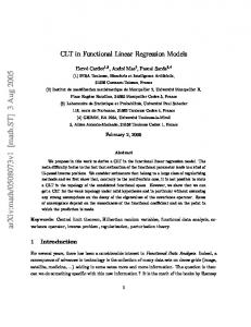
Figure 4: Screening simulation results for the case (σe2 , sn ) = (1, 2000): the curves of percentage of the average true nonzero coverage proportion. The black solid, blue dashed, red dotted, and purple dashed dotted lines correspond to the rank-one screening, the L1 entrywise norm screening, the Frobenius norm screening, and the global Wald test screening, respectively. Panels (a)-(i) correspond to (n, ps , qs ) = (100, 4, 4), (200, 4, 4), (500, 4, 4), (100, 8, 8), (200, 8, 8), (500, 8, 8), (100, 16, 16), (200, 16, 16), and (500, 16, 16), respectively.

24

0.4

0.7

0.35

0.6

0.9

0.8

Nonzero Coverage Proportions

Nonzero Coverage Proportions

0.25

0.2

0.15

Nonzero Coverage Proportions

0.7 0.3

0.5

0.4

0.3

0.2

0.1

0.5

0.4

0.3

0.2 0.1

0.05

0

0.6

0.1

0

20

40

60

80

100

120

140

160

180

0

200

0

20

40

60

80

100

120

140

160

180

0

200

0

20

40

60

Threshold value

Threshold value

(a)

100

120

140

160

180

200

140

160

180

200

140

160

180

200

Threshold value

(b)

0.6

80

(c)

0.8

1

0.9

0.7 0.5

0.8

0.4

0.3

0.2

Nonzero Coverage Proportions

Nonzero Coverage Proportions

Nonzero Coverage Proportions

0.6

0.5

0.4

0.3

0.7

0.6

0.5

0.4

0.3

0.2 0.2 0.1 0.1

0

0

20

40

60

80

100

120

140

160

180

0

200

0.1

0

20

40

60

Threshold value

80

100

120

140

160

180

0

200

0

20

40

60

Threshold value

(d)

100

120

Threshold value

(e)

0.6

80

(f)

0.8

1

0.9

0.7 0.5

0.8

0.4

0.3

0.2

Nonzero Coverage Proportions

Nonzero Coverage Proportions

Nonzero Coverage Proportions

0.6

0.5

0.4

0.3

0.7

0.6

0.5

0.4

0.3

0.2 0.2 0.1 0.1

0

0

20

40

60

80

100

120

140

160

180

200

0

0.1

0

20

40

60

80

100

120

Threshold value

Threshold value

(g)

(h)

140

160

180

200

0

0

20

40

60

80

100

120

Threshold value

(i)

Figure 5: Screening simulation results for the case (σe2 , sn ) = (25, 2000): the curves of percentage of the average true nonzero coverage proportion. The black solid, blue dashed, red dotted, and purple dashed dotted lines correspond to the rank-one screening, the L1 entrywise norm screening, the Frobenius norm screening, and the global Wald test screening, respectively. Panels (a)-(i) correspond to (n, ps , qs ) = (100, 4, 4), (200, 4, 4), (500, 4, 4), (100, 8, 8), (200, 8, 8), (500, 8, 8), (100, 16, 16), (200, 16, 16), and (500, 16, 16), respectively.

25

our screening procedure based on the random decoupling and then apply our regularized b l (l = 1, 2, 3, 4), model size, and low rank estimation procedure. We report the MSEs of B prediction error based on 100 replications in Table 3. We report the proportion of times that we exactly select the true model M = {1, 2, 3, 4}, the proportion that we over-select some variables, but include all the true ones, and the proportion that we miss some of the important covariates in Table 4. The proposed random decoupling works well in choosing γn , since the selected covariate set based on γn includes the true covariates with high probabilities in all scenarios. Second, we consider over-selecting and/or missing some covariates. For each of the three b l (l = 1, 2, 3, 4) and the prediction error in Table above cases, we report the MSEs of B 4. When the screening procedure over-selects more irrelevant variables, the MSEs of the true non-zero coefficient matrices and prediction error of the fitted model are similar to those obtained from the model with the correct set of covariates. In contrast, if the screening procedure misses several important variables, then the estimates corresponding to these missed variables completely fail since the corresponding coefficient matrices are estimated zero. However, according to the simulation results, the MSEs corresponding to those important variables that have been selected, are similar to those obtained from the model with the correct set of covariates. The prediction error increases due to missing some important variables. Table 3: The means of predictor errors (PEs) and MSEs for our two-step procedure, and the average selected model size for our screening procedure. Their associated standard errors are in the parentheses. For each case, 100 simulated data sets are used. (n, sn , σe2 )

MSE(B1 )

MSE(B2 )

MSE(B3 )

MSE(B4 )

PE

Model Size

(100, 2000, 1)

15.87(3.22)

10.73(0.67)

43.52(0.46)

47.07(0.58)

1.05(0.001)

5.24(0.11)

(200, 2000, 1)

5.92(0.10)

5.10(0.11)

27.61(0.27)

28.23(0.31)

1.03(0.0003)

5.87(0.11)

(100, 5000, 1)

32.28(6.57)

12.60(1.08)

44.28(0.52)

47.14(0.65)

1.07(0.002)

5.03(0.10)

(200, 5000, 1)

5.92(0.09)

4.94(0.09)

28.03(0.29)

28.35(0.29)

1.03(0.0005)

5.83(0.13)

(100, 2000, 25)

126.17(1.84)

119.15(2.56) 227.86(1.96)

279.22(3.17)

25.99(0.027)

5.15(0.11)

(200, 2000, 25)

84.42(1.25)

73.69(1.41)

177.90(1.66)

214.67(2.15)

25.54(0.012)

5.82(0.11)

(100, 5000, 25)

136.27(3.45)

118.73(2.63) 228.65(2.19)

278.43(3.42)

26.04(0.024)

4.96(0.11)

(200, 5000, 25)

82.69(1.12)

73.53(1.37)

211.25(2.12)

25.56(0.012)

5.75(0.13)

177.44(1.57)

26

5

The Philadelphia Neurodevelopmental Cohort

5.1

Data Description and Preprocessing Pipeline

To motivate the proposed methodology, we consider a large database with imaging, genetic, and clinical data collected by the Philadelphia Neurodevelopmental Cohort (PNC) study. This study was a collaboration between the Center for Applied Genomics (CAG) at Children’s Hospital of Philadelphia (CHOP) and the Brain Behavior Laboratory at the University of Pennsylvania (Penn). The PNC cohort consists of youths aged 8-21 years in the CHOP network and volunteered to participate in genomic studies of complex pediatric disorders. All participants underwent clinical assessment and a neuroscience based computerized neurocognitive battery (CNB) and a subsample underwent neuroimaging. We consider 814 subjects with 429 females and 385 males. The age range of the 814 participants is 8-21 (years) with mean value 14.36 (years) and standard deviation 3.48 (years). Specifically, each subject has a resting state functional magnetic resonance imaging (rs-fMRI) connectivity matrix, which is represented as a 69×69 matrix, and a large genetic data set with around 5, 400, 000 genotyped and imputed single-nucleotide polymorphisms (SNPs) on all of the 22 chromosomes. Other clinical variables of interest include age and gender, among others. Our primary question of interest is to identify novel genetic effects on the local rs-fMRI connectivity changes. We preprocess the resting state fMRI data using C-PAC pipeline. First, we register the fMRI data to the standard MNI 2mm resolution level and perform segmentation using the CPAC default setting. Next, we do motion correction using the Friston 24-parameter method. We also perform nuisance signal correction by regressing out the following variables: top 5 principle components in the noise regions of interest (ROIs), Cerebrospinal fluid (CSF), motion parameters, and the linear trends in time series. Finally, we extract the ROI time series by taking the average of voxel-wise time series in each ROI. The atlases that we use are HarvardOxford Cortical Atlas (48 regions) and HarvardOxford Subcortical Atlas (21 regions), which could be found in FSL. In total, we extract time series for each of the 69 regions and each time series has 120 observations after deleting the first and last 3 scans.

27

Table 4: The means of PEs and MSEs for our two-step procedure in three scenarios: exact selection (“Exact”), over selection (“Over”) and missing variables (“Miss”). The proportion of times among 100 simulated data sets for each scenario is also reported. The “NA” denotes the values that are not applicable. (n, sn , σe2 )

Scenario

MSE(B1 )

MSE(B2 )

MSE(B3 )

MSE(B4 )

PE

Proportion

(100, 2000, 1)

Exact

11.61(0.18)

9.18(0.16)

43.22(0.38)

45.55(0.47)

1.06(0.001)

0.27

Over

11.17(0.17)

10.11(0.20)

43.6(0.46)

47.31(0.56)

1.05(0.001)

0.71

Miss

240(0)

53.49(1.68)

44.58(1.61)

59.11(1.18)

1.10(0.001)

0.02

Exact

7.09(0.08)

6.6(0.12)

23.97(0.16)

23.11(0.09)

1.03(0.0005)

0.04

Over

5.87(0.09)

5.03(0.11)

27.76(0.26)

28.44(0.30)

1.03(0.0003)

0.96

Miss

NA

NA

NA

NA

NA

0

Exact

11.69(0.17)

9.74(0.19)

44.14(0.65)

45.79(0.41)

1.07(0.001)

0.27

Over

11.76(0.20)

9.75(0.19)

44.24(0.43)

46.60(0.54)

1.06(0.001)

0.64

Miss

240(0)

41.48(1.93)

44.96(0.65)

55.10(1.23)

1.12(0.001)

0.09

Exact

7.52(0.09)

6.69(0.11)

24.91(0.22)

24.24(0.08)

1.04(0.001)

0.05

Over

5.84(0.08)

4.84(0.08)

28.19(0.28)

28.57(0.28)

1.03(0.0005)

0.95

Miss

NA

NA

NA

NA

NA

0

(200, 2000, 1)

(100, 5000, 1)

(200, 5000, 1)

(100, 2000, 25)

(200, 2000, 25)

(100, 5000, 25)

(200, 5000, 25)

Exact

121.75(1.27) 114.12(2.19)

Over

126.37(1.49)

Miss

229.79(1.95)

270.16(3.47) 26.18(0.024)

0.29

121.47(2.69) 227.21(1.98)

283.29(3.00)

25.91(0.023)

0.70

240(NA)

102.16(NA)

217.49(NA)

256.52(NA)

26.45(NA)

0.01

Exact

79.26(0.80)

64.22(0.61)

177.62(0.86)

207.41(1.18) 25.54(0.017)

Over

84.81(1.27)

74.4(1.43)

177.92(1.71) 215.21(2.20)

Miss

NA

NA

NA

Exact

122.88(1.74)

114.5(2.49)

Over

129.81(1.53)

Miss

0.07

25.54(0.012)

0.93

NA

NA

0

217.93(1.87)

260.99(2.64)

26.20(0.019)

0.34

122.59(2.63) 233.46(2.17)

286.15(3.34)

25.92(0.020)

0.58

240(0)

108.61(3.01)

239.31(2.06)

296.51(4.25) 26.23(0.022)

0.08

Exact

85.2(0.87)

72.92(1.48)

174.83(1.20)

206.34(2.32)

25.66(0.014)

0.06

Over

82.53(1.14)

73.57(1.37)

177.61(1.60)

211.56(2.12)

25.55(0.012)

0.94

Miss

NA

NA

NA

NA

NA

0

28

5.2

Analysis and Results

We first fit model (1) with the rs-fMRI connectivity matrices from 814 subjects as 69 × 69 matrix responses and age and gender as clinical covariates. We also include the first 5 principal component scores based on the SNP data as covariates to correct for population stratification. We first calculate the ordinary least squares estimates of coefficient matrices and then compute the corresponding residual matrices for the brain connectivity response matrix after adjusting the effects of the clinical covariates and the SNP principal component scores. Second, we apply the rank-one screening procedure by using the residual matrices as responses to select important SNPs from the whole set of 5, 354, 265 SNPs that are highly associated with the residual matrices. We use the random decoupling method described in b l kop Section 2.1 to choose the thresholding value γn and select all those indices whose kB is the larger than γn . Finally, seven covariates are selected, where the names are shown in Table 5. Among these seven SNPS, the first three ones on Chromosome 5 have exactly the same genotypes for all the subjects and the next four ones on Chromosome 10 have exactly the same genotypes for all the subjects. Table 5: PNC data analysis results: the top 7 SNPs selected by our screening procedure. Ranking

Chromosome

SNP

1

5

rs72775042

2

5

rs6881067

3

5

rs72775059

4

10

rs200328746

5

10

rs75860012

6

10

rs200248696

7

10

rs78309702

Finally, we examine the effects of these selected SNPs on our matrix response. We first fit the OLS to these 7 SNPs. Since the first three ones have exactly the same genotypes and the next four ones have exactly the same genotypes, we regress our matrix response on 29

the first selected SNP and the fourth selected SNP, yielding two coefficient matrix estimates b ols . The OLS estimates for the 7 SNPs are defined as B b ols = B b ols = B b ols = B b ols /3 b ols and B B 1 2 3 (1) (2) (1) b ols /4. We then calculate the singular values of these b ols = B b ols = B b ols = B b ols = B and B 7 6 5 4 (2) 7 OLS estimates and plot these singular values in decreasing order in Figure 6. Inspecting Figure 6 reveals that these estimated coefficient matrices have a clear low rank pattern since the first few singular values dominate the remaining ones. This motivates us to apply our RLR estimation procedure to estimate the coefficient matrices corresponding to these 7 SNP covariates. Figure 7(a)-(g) presents the coefficient matrix estimates associated with these SNPs. The coefficient matrices corresponding to the first three selected SNPs are the same and the coefficient matrices corresponding to next four selected SNPs are the same. The estimated ranks of these seven coefficient matrices are given by 11, 11, 11, 8, 8, 8, and 8, respectively.

6

Discussion

Motivated from the analysis of imaging genetic data, we have proposed a low-rank linear regression model to correlate high-dimensional matrix responses with a high dimensional vector of covariates when coefficient matrices are approximately low-rank. We have developed a fast and efficient rank-one screening procedure, which enjoys the sure independence screening property as well as vanishing false selection rate, to reduce the covariate space. We have developed a regularized estimate of coefficient matrices based on the trace norm regularization, which explicitly incorporates the low-rank structure of coefficient matrices, and established its estimation consistency. We have further established a theoretical guarantee for the overall solution obtained from our two-step screening and estimation procedure. We have demonstrated the efficiency of our methods by using simulations and the analysis of PNC dataset.

30

(a)

(b)

(c)

(d)

(e)

(f)

(g)

Figure 6: PNC data: Panel (a)-(g) are the plots for the singular values of the OLS estimates corresponding to the 7 SNPs selected by our screening step, with singular values sorted from largest to smallest.

31

(a)

(b)

(c)

(d)

(e)

(f)

(g)

Figure 7: PNC data: Panel (a)-(g) are the plots for our RLR estimates corresponding to the 7 SNPs selected by our screening step.

32

References Bach, F. R. (2008), “Consistency of trace norm minimization,” Journal of Machine Learning Research, 9, 1019–1048. Barrett, J. C., Fry, B., Maller, J., and Daly, M. J. (2005), “Haploview: analysis and visualization of LD and haplotype maps,” Bioinformatics, 21, 263–265. Barut, E., Fan, J., and Verhasselt, A. (2016), “Conditional sure independence screening,” Journal of the American Statistical Association, 111, 1266–1277. Beck, A. and Teboulle, M. (2009), “A fast iterative shrinkage-thresholding algorithm for linear inverse problems,” SIAM Journal on Imaging Sciences, 2, 183–202. Breiman, L. and Friedman, J. (1997), “Predicting multivariate responses in multiple linear regression,” Journal of the Royal Statistical Society, 59, 3–54. Buhlmann, P. and van de Geer, S. (2011), Statistics for High-Dimensional Data: Methods, Theory and Applications., New York, N. Y.: Springer. Cai, J.-F., Cand`es, E. J., and Shen, Z. (2010), “A singular value thresholding algorithm for matrix completion,” SIAM Journal on Optimization, 20, 1956–1982. Candes, E. and Tao, T. (2007), “The Dantzig selector: Statistical estimation when p is much larger than n,” The Annals of Statistics, 2313–2351. Cand`es, E. J. and Recht, B. (2009), “Exact matrix completion via convex optimization,” Foundations of Computational Mathematics., 9, 717–772. Chen, Y., Goldsmith, J., and Ogden, T. (2016), “Variable Selection in Function-on-Scalar Regression,” Stat, 5, 88–101. Chiang, M. C., Barysheva, M., Toga, A. W., Medland, S. E., Hansell, N. K., James, M. R., McMahon, K. L., de Zubicaray, G. I., Martin, N. G., Wright, M. J., and Thompson, P. M. (2011), “BDNF gene effects on brain circuitry replicated in 455 twins,” NeuroImage, 55, 448–454. 33

Cook, R., Helland, I., and Su, Z. (2013), “Envelopes and partial least squares regression,” Journal of the Royal Statistical Society: Series B (Statistical Methodology), 75, 851–877. Ding, S. and Cook, D. (2018), “Matrix variate regressions and envelope models,” Journal of the Royal Statistical Society: Series B (Statistical Methodology), 80, 387–408. Ding, S. and Cook, R. D. (2014), “Dimension folding PCA and PFC for matrix-valued predictors,” Statistica Sinica, 24, 463–492. Facchinei, F. and Pang, J.-S. (2003), Finite-dimensional variational inequalities and complementarity problems. Vol. I, Springer Series in Operations Research, Springer-Verlag, New York. Fan, J., Feng, Y., and Song, R. (2011), “Nonparametric independence screening in sparse ultra-high-dimensional additive models,” Journal of the American Statistical Association, 106, 544–557. Fan, J. and Lv, J. (2008), “Sure independence screening for ultrahigh dimensional feature space,” Journal of the Royal Statistical Society. Series B., 70, 849–911. — (2010), “A selective overview of variable selection in high dimensional feature space,” Statistica Sinica, 20, 101. Fan, J. and Song, R. (2010), “Sure independence screening in generalized linear models with NP-dimensionality,” The Annals of Statistics, 38, 3567–3604. Fosdick, B. K. and Hoff, P. D. (2015), “Testing and modeling dependencies between a network and nodal attributes,” Journal of the American Statistical Association, 110, 1047–1056. Gabriel, S. B., Schaffner, S. F., Nguyen, H., Moore, J. M., Roy, J., Blumenstiel, B., Higgins, J., DeFelice, M., Lochner, A., Faggart, M., et al. (2002), “The structure of haplotype blocks in the human genome,” Science, 296, 2225–2229. Hibar, D., Stein, J. L., Kohannim, O., Jahanshad, N., Saykin, A. J., Shen, L., Kim, S., Pankratz, N., Foroud, T., Huentelman, M. J., Potkin, S. G., Jack, C., Weiner, M. W., Toga, A. W., Thompson, P., and ADNI (2011), “Voxelwise gene-wide association study 34

(vGeneWAS): multivariate gene-based association testing in 731 elderly subjects,” NeuroImage, 56, 1875–1891. Huang, M., Nichols, T., Huang, C., Yang, Y., Lu, Z., Feng, Q., Knickmeyer, R. C., Zhu, H., and ADNI (2015), “FVGWAS: Fast Voxelwise Genome Wide Association Analysis of Large-scale Imaging Genetic Data,” NeuroImage, 118, 613–627. Leng, C. and Tang, C. Y. (2012), “Sparse matrix graphical models,” Journal of the American Statistical Association, 107, 1187–1200. Li, L. and Zhang, X. (2017), “Parsimonious tensor response regression,” Journal of the American Statistical Association, 112, 1131–1146. Liu, J. and Calhoun, V. D. (2014), “A review of multivariate analyses in imaging genetics,” Frontiers in Neuroinformatics, 8, 29. Medlan, S. E., Jahanshad, N., Neale, B. M., and Thompson, P. M. (2014), “Whole-genome analyses of whole-brain data: working within an expanded search space,” Nature Neuroscience, 17, 791–800. Medland, S. E., Jahanshad, N., Neale, B. M., and Thompson, P. M. (2014), “Whole-genome analyses of whole-brain data: working within an expanded search space,” Nature Neuroscience, 17, 791–800. Negahban, S., Yu, B., Wainwright, M. J., and Ravikumar, P. K. (2009), “A unified framework for high-dimensional analysis of M -estimators with decomposable regularizers,” in Advances in Neural Information Processing Systems, pp. 1348–1356. Negahban, S. N., Ravikumar, P., Wainwright, M. J., and Yu, B. (2012), “A unified framework for high-dimensional analysis of M -estimators with decomposable regularizers,” Statistical Science, 27, 538–557. Nesterov, Y. (2004), Introductory lectures on convex optimization, vol. 87 of Applied Optimization, Kluwer Academic Publishers, Boston, MA, a basic course.

35

Park, Y., Su, Z., and Zhu, H. (2017), “Groupwise envelope models for imaging genetic analysis,” Biometrics, 73, 1243–1253. Peng, J., Zhu, J., Bergamaschi, A., Han, W., Noh, D. Y., Pollack, J. R., and Wang, P. (2010), “Regularized multivariate regression for identifying master predictors with application to integrative genomics study of breast cancer,” Annals of Applied Statistics, 4, 53–77. Peper, J. S., Brouwer, R. M., Boomsma, D. I., Kahn, R. S., and Pol, H. E. H. (2007), “Genetic Influences on Human Brain Structure: A Review of Brain Imaging Studies in Twins,” Human Brain Mapping, 28, 464–473. Purcell, S., Neale, B., Todd-Brown, K., Thomas, L., Ferreira, M. A., Bender, D., Maller, J., Sklar, P., De Bakker, P. I., Daly, M. J., et al. (2007), “PLINK: a tool set for wholegenome association and population-based linkage analyses,” The American Journal of Human Genetics, 81, 559–575. Rabusseau, G. and Kadri, H. (2016), “Low-rank regression with tensor responses,” in Advances in Neural Information Processing Systems, pp. 1867–1875. Ramsay, J. O. and Silverman, B. W. (2005), Functional Data Analysis, New York, N. Y.: Springer, 2nd ed. Raskutti, G. and Yuan, M. (2018), “Convex regularization for high-dimensional tensor regression,” Annals of Statistics, to appear. Scharinger, C., Rabl, U., Sitte, H. H., and Pezawas, L. (2010), “Imaging genetics of mood disorders,” NeuroImage, 53, 810–821. Shen, L., Kim, S., Risacher, S. L., Nho, K., Swaminathan, S., West, J. D., Foroud, T., Pankratz, N., Moore, J. H., Sloan, C. D., Huentelman, M. J., Craig, D. W., DeChairo, B. M., Potkin, S. G., Jr, C. R. J., Weiner, M. W., Saykin, A. J., and ADNI (2010), “Whole genome association study of brain-wide imaging phenotypes for identifying quantitative trait loci in MCI and AD: A study of the ADNI cohort,” NeuroImage, 53, 1051–1063.

36

Stein, J., Hua, X., Lee, S., Ho, A., Leow, A., Toga, A., Saykin, A. J., Shen, L., Foroud, T., Pankratz, N., Huentelman, M., Craig, D., Gerber, J., Allen, A., Corneveaux, J. J., Dechairo, B., Potkin, S., Weiner, M., Thompson, P., and ADNI (2010), “Voxelwise genome-wide association study (vGWAS),” NeuroImage, 53, 1160–1174. Thompson, P. M., Ge, T., Glahn, D. C., Jahanshad, N., and Nichols, T. E. (2013), “Genetics of the connectome,” NeuroImage, 80, 475–488. Thompson, P. M., Stein, J. L., Medland, S. E., Hibar, D. P., Vasquez, A. A., Renteria, M. E., Toro, R., Jahanshad, N., Schumann, G., Franke, B., et al. (2014), “The ENIGMA Consortium: large-scale collaborative analyses of neuroimaging and genetic data,” Brain Imaging and Behavior, 8, 153–182. Tibshirani, R. (1997), “The lasso method for variable selection in the Cox model,” Statistics in Medicine, 16, 385–395. Vounou, M., Janousova, E., Wolz, R., Stein, J., Thompson, P., Rueckert, D., Montana, G., and ADNI (2012), “Sparse reduced-rank regression detects genetic associations with voxel-wise longitudinal phenotypes in Alzheimer’s disease,” NeuroImage, 60, 700–716. Vounou, M., Nichols, T. E., Montana, G., and ADNI (2010), “Discovering genetic associations with high-dimensional neuroimaging phenotypes: A sparse reduced-rank regression approach,” NeuroImage, 53, 1147–1159. Wang, H., Nie, F., Huang, H., Kim, S., Nho, K., Risacher, S., Saykin, A., Shen, L., and ADNI (2012a), “Identifying quantitative trait loci via group-sparse multi-task regression and feature selection: An imaging genetics study of the ADNI cohort,” Bioinformatics, 28, 229–237. Wang, H., Nie, F., Huang, H., Risacher, S., Saykin, A., Shen, L., and ADNI (2012b), “Identifying disease sensitive and quantitative trait relevant biomarkers from multi-dimensional heterogeneous imaging genetics data via sparse multi-modal multi-task learning,” Bioinformatics, 28, 127–136.

37

Wang, L., Chen, G., and Li, H. (2007), “Group SCAD regression analysis for microarray time course gene expression data,” Bioinformatics, 23, 1486–1494. Yuan, M., Ekici, A., Lu, Z., and Monteiro, R. (2007), “Dimension reduction and coefficient estimation in multivariate linear regression,” Journal of the Royal Statistical Society. Series B., 69, 329–346. Zhang, Y. W., Xu, Z. Y., Shen, X. T., and Pan, W. (2014), “Testing for association with multiple traits in generalized estimation equations, with application to neuroimaging data,” NeuroImage, 96, 309–325. Zhao, J. and Leng, C. (2014), “Sparse matrix graphical models,” Statistica Sinica, 24, 799– 814. Zhao, P. and Yu, B. (2006), “On model selection consistency of Lasso,” Journal of Machine Learning Research, 7, 2541–2563. Zhou, H. and Li, L. (2014), “Regularized matrix regression,” Journal of the Royal Statistical Society. Series B., 76, 463–483. Zhu, H., Khondker, Z. S., Lu, Z., and Ibrahim, J. G. (2014), “Bayesian generalized low rank regression models for neuroimaging phenotypes and genetic markers,” Journal of American Statistical Association, 109, 977–990. Zou, H. (2006), “The adaptive lasso and its oracle properties,” Journal of the American Statistical Association, 101, 1418–1429.

38