The Astrophysical Journal, 496:L93–L96, 1998 April 1 q 1998. The American Astronomical Society. All rights reserved. Printed in U.S.A.
MORPHOLOGICAL NUMBER COUNTS AND REDSHIFT DISTRIBUTIONS TO I ! 26 FROM THE HUBBLE DEEP FIELD: IMPLICATIONS FOR THE EVOLUTION OF ELLIPTICALS, SPIRALS, AND IRREGULARS S. P. Driver, A. Ferna´ndez-Soto, and W. J. Couch School of Physics, University of New South Wales, Sydney, NSW 2052, Australia
S. C. Odewahn Department of Astronomy, California Institute of Technology, Pasadena, CA 91125
R. A. Windhorst Department of Physics and Astronomy, Arizona State University, Box 871504, Tempe, AZ 85287-1504
S. Phillipps Astrophysics Group, Department of Physics, University of Bristol, Tyndall Avenue, Bristol BS8 1TL, England, UK
and K. Lanzetta and A. Yahil Department of Physics and Astronomy, State University of New York at Stony Brook, Stony Brook, NY 11794-2100 Received 1997 December 5; accepted 1998 February 5; published 1998 March 11
ABSTRACT We combine the photometric redshift data of Ferna´ndez-Soto et al. with the morphological data of Odewahn et al. for all galaxies with I ! 26.0 detected in the Hubble Deep Field. From this combined catalog we generate the morphological galaxy number counts and corresponding redshift distributions and compare these to the predictions of high-normalization zero- and passive-evolution models. From this comparison we conclude the following: 1. E/S0’s are seen in numbers and over a redshift range consistent with zero-evolution or minimal passiveevolution to I 5 24. Beyond this limit, fewer E/S0’s are observed than predicted implying a net negative evolutionary process—luminosity dimming, disassembly or masking by dust—at I 1 24 . The breadth of the redshift distribution at faint magnitudes implies strong clustering or an extended epoch of formation commencing at z 1 3. 2. Spiral galaxies are present in numbers consistent with zero-evolution predictions to I 5 22 . Beyond this magnitude some net positive evolution is required. Although the number counts are consistent with the passiveevolution predictions to I 5 26.0 , the redshift distributions favor number and luminosity evolution, although few obvious mergers are seen (possibly classified as irregulars). We note that beyond z ∼ 2 very few ordered spirals are seen suggesting a formation epoch of spiral galaxies at z ∼ 1.5–2. 3. There is no obvious explanation for the late-type/irregular class, and this category requires further subdivision. While a small fraction of the population lies at low redshift (i.e., true irregulars), the majority lie at redshifts 1 ! z ! 3. At z 1 1.5 mergers are frequent and, taken in conjunction with the absence of normal spirals at z 1 2, the logical inference is that they represent the progenitors of normal spirals that form via hierarchical merging. Subject headings: galaxies: elliptical and lenticular, cD — galaxies: evolution — galaxies: irregular — galaxies: spiral dwarf-dominated models, pure luminosity evolution models, and merger models. All of these various models can provide a fit to the observed faint galaxy number counts, and therefore these data alone are insufficient to distinguish between the proposed models. Additional observational constraints are required, and the most definitive one is that of the observed redshift distributions, N(z), for progressively fainter magnitude slices. For example, dwarf-dominated models (Driver et al. 1994; Phillipps & Driver 1995; Babul & Ferguson 1996) predict an additional low-redshift component at faint magnitudes when compared with the N(z) predictions of the zero-evolution models. Conversely, pure luminosity evolution models (see, e.g., Metcalfe et al. 1995; Campos & Shanks 1997) predict a high-redshift component, while merger models lie somewhere in between (see, e.g., Carlberg 1992; Rocca-Volmerange & Guiderdoni 1990). In theory, then, the problem is surmount-
1. INTRODUCTION
The Hubble Deep Field (HDF; Williams et al. 1996) has provided the deepest and clearest window to date on the extragalactic sky. From this data set, groups have studied the morphologies of the faintest galaxies (see, e.g., Odewahn et al. 1996; Abraham et al. 1996) and made photometric estimates of the redshift of these objects (see, e.g., Lanzetta, Yahil, & Ferna´ndez-Soto 1996; Brunner et al. 1997). Here we combine these two independent analyses to generate morphological number counts and morphological redshift distributions for a complete sample of objects from the Hubble Deep Field (413 objects to I 5 26.0). This represents a unique data set that provides strong constraints on the many faint galaxy models that have been postulated to explain the phenomena of the faint blue excess (see Ellis 1997 for a recent review). Faint galaxy models fall into three broad generic categories: L93
L94
DRIVER ET AL.
Vol. 496
able; in practice, obtaining a comprehensive and complete spectroscopic redshift distribution at faint magnitudes is beyond our technological capabilities. The very faint redshift surveys that do exist (see, e.g., Glazebrook et al. 1995a; Cowie et al. 1996) are relatively small samples and are arguably susceptible to selection biases (e.g., wavelength coverage, spectral features, surface brightness). For the moment, the only recourse for establishing the N(z) distribution at these faint magnitudes is to utilize distance estimates based on multiband photometry, i.e., photometric redshifts. In § 2, we briefly discuss the adopted morphological and photometric HDF catalogs. In § 3, we compare the resulting galaxy number count data and redshift distributions with zeroand passive-evolution models and infer the generic form of evolution implied by the data. Section 4 summarizes our findings. 2. THE CATALOGS
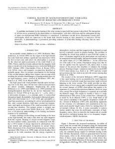
In recent years the high-resolution imaging provided by the Wide Field and Planetary Camera 2 on the Hubble Space Telescope (HST) has opened up the new field of the morphological classification of faint galaxies. The initial work relied on the eyeball consensus of a number of experienced galaxy classifiers to subdivide the faint galaxy population into ellipticals (E/S0’s), early-type spirals (Sabc’s), and late-type spirals/irregulars (Sd/ Irr’s) (see, e.g., Driver, Windhorst, & Griffiths 1995a; Driver et al. 1995b; Glazebrook et al. 1995b). The primary motivation for subdividing into these three categories was based on the existence of observable structural distinctions between these broad groupings (e.g., de Vaucouleurs, exponential, or asymmetric profiles for E/S0, Sabc, or Sd/Irr, respectively). In addition, the E/S0 and Sabc classes are also known to have distinct physical properties (i.e., pressure or rotationally supported components). If these differing structural and physical properties are the result of independent evolutionary paths, then this provides a justification for studying their number density evolution independently. Ultimately, automated methods are required to construct statically representative samples in a fully reproducible and objective manner. This approach has generally taken two paths: artificial neural networks (ANN; see Odewahn et al. 1996; Naim et al. 1995) and decision trees based on structural parameters (e.g., Casertano et al. 1995; Abraham et al. 1996). Both techniques show promise, performing at a level close to that of eyeball classification but occasionally seen to fail when dealing with objects with overlapping isophotes. To overcome this potential bias, we initially adopt the HDF catalog generated by the ANN of Odewahn et al. (1996) and compare it with the results from the eyeball classifications of one of us (W. J. C.).1 Figure 1 shows the resulting histogram distribution of DT-types and can be approximated by a Gaussian of mean 0.1 5 0.2 and FWHM 1.5 5 0.2. However, the wings are nonGaussian, suggesting that where there is disagreement it tends to be large and systematic. Examining only those images for which the T-type differences are large, we see that it is routinely the ANN that has failed and that the majority of these discrepancies are unambiguous cases of extreme irregularity, mergers, or bright cores embedded in irregular halos. This is not surprising, since there were few such objects in the ANNs original training set (based on brighter galaxies in less deep fields, cf. Odewahn et al. 1996). To accommodate this, we 1
Note that the ANN was originally trained on data classified by S. C. O., R. A. W., and S. P. D., and hence, this represents an unbiased and independent check of the classification accuracy.
Fig. 1.—The DT-type histogram for the full sample (solid line) and the faintest magnitude bin only (dashed line).
constructed a final catalog in which the initial blind ANN classifications were replaced by the eyeball classification if the Ttype disagreement was greater than four T-types (i.e., where the histogram in Fig. 1 becomes asymmetric). This resulted in 20% of the original ANN HDF galaxy classifications being overridden. Also shown in Figure 1 is the DT-type histogram for the faintest magnitude bin (25 ! I ! 26 ), and we note that the distribution is similar to that of the entire sample, implying little or no degradation in classification accuracy with apparent magnitude. The photometric redshift catalog (described in more detail in Ferna´ndez-Soto, Lanzetta, & Yahil 1998) is based on that presented in Lanzetta et al. (1996), but it has been updated to take advantage of ground-based IR images of the HDF (Dickinson et al. 1998). The determination of the photometric redshifts are obtained by maximizing the likelihood function L(z, T ). The likelihood L(z, T ) of obtaining measured fluxes fi with uncertainties ji given modeled fluxes Fi(z, T) for a given spectral type T at redshift z, with a flux normalization A over the seven filters (i 5 1–7) is
P { [ 7
L(z, T ) 5
i51
exp 2
1 fi 2 AFi (z, T ) 2 ji
2
]}
.
This formula is maximized for each of four possible spectral types for each object. This results in four redshift likelihood functions L(z), which are simultaneously maximized to give both the optimal redshift and the spectral classification. The four model templates [Fi(z, T)] were adopted from Coleman, Wu, & Weedman (1980) and extended to the infrared wavelengths using the models of Bruzual & Charlot (1993). Intergalactic H i absorption was taken into account in the same way as described in Lanzetta et al. (1996). Details of the method and the reliability of the photometric redshifts are discussed in full in Ferna´ndez-Soto et al. (1998). To summarize, the agreement between the photometric and the known spectroscopic redshifts is excellent in the low-redshift range (z ! 1.5 ), where
No. 2, 1998
MORPHOLOGICAL NUMBER COUNTS
Fig. 4.—Number counts for the different morphological types: all galaxies (upper left), E/S0 (upper right), Sabc (lower left), and Sd/Irr (lower right). Data are from Casertano et al. (1995) (CRGINOW), Driver et al. (1995a) (DWG), Driver et al. (1995b) (DWOKGR), and this study (HDF). The number count predictions of the zero- and passive-evolution models are shown as solid and dashed lines, respectively.
the rms deviation is D(z spec 2 z phot ) rms ≈ 0.15 with no measurable bias in the residual distribution. At z 1 2, some discordant values are seen (less than 10%), and we note that the redshifts tend to underestimate the real values in the range 2 ! z ! 3. No trend in Dz with T-type was seen. For objects where spectroscopic redshifts were available, these were used instead of the photometric values. The final catalog is therefore based on 20% spectroscopic and 80% photometric redshifts; however, we note that the agreement between spectroscopic and photometric redshifts are extremely good (cf. Hogg et al. 1998), and the results are unchanged if purely photometric redshifts are used. The morphological and photometric redshift catalogs were merged by matching the x- and y-positions of the two catalogs. While the majority of objects were successfully matched, a small fraction (∼5%) failed. These miscreants were traced to either positional discrepancies or differences in the deblending of complex structures; in these cases deference was once again given to the eyeballed classifications. The final matched catalog contains 401 objects with z’s and morphologies to I 5 26 and a further 12 with morphologies only (i.e., a reliable photometric redshift was not measured or not measurable). True color representations of the full final catalog ordered according to morphology (Fig. 2 [Pl. L7]) and redshift (Fig. 3 [Pl. L8]) are shown. Of particular interest in Figure 3 is the trend toward higher irregularity and/or a higher merger rate beyond z ∼ 1.5 (coincident with the peak in the star formation rate as reported in Madau et al. 1996). Qualitatively, at least this visually suggests a universe at z 1 1.5 dominated by a period of hierarchical merging of star-forming irregular galaxy clumps (cf. Pascarelle et al. 1996). 3. MORPHOLOGICAL N(m) AND N(z)s
Figures 4 and 5 show the morphological number counts and morphological redshift distributions, respectively. The zeroevolution model predictions are shown as solid lines, while the
L95
Fig. 5.—Morphological redshift distributions for 22 ! I ! 23 (top), 23 ! I ! 24 (upper middle), 24 ! I ! 25 (lower middle), and 25 ! I ! 26 (bottom). The columns are, from left to right: all galaxies, E/S0’s, Sabc’s, and Sd/Irr’s. Overlaid are the zero-evolution (solid line) and passive-evolution (dashed line) model predictions.
passive-evolution predictions are shown as dashed lines. These models are based on the following: the local morphological luminosity distributions of Marzke et al. (1994), the k- and evolutionary-corrections of Poggianti (1997), a standard flat cosmology (i.e., q0 5 0.5, L 5 0), and a global renormalization (#1.8) of the local galaxy numbers based on an optimal count match at bJ 5 18.0 (more detail on the modeling is given in Driver et al. 1995b). Considering each population independently, we note the following. E/S0’s.—At brighter magnitudes (I ! 24 ), both the counts and the redshift distributions agree well with the predictions of the zero-evolution model, implying little net evolution (see, e.g., Driver et al. 1996 for discussion of the counteracting effects of luminosity and number evolution). At fainter magnitudes (24 ! I ! 26), there is a marginally significant (2 j) shortfall in the counts compared with the models. This may be a statistical fluctuation2 or a pointer toward a net negative evolutionary process or a higher dust content than allowed for in the models (see, e.g., Campos & Shanks 1997). If it is real, the shortfall may indicate a modest rate of continued formation of some extra ellipticals via mergers (see, e.g., Zepf 1997; Zeigler & Bender 1997). These conclusions from the counts appear to be in good agreement with those obtained from direct structural (fundamental plane) and spectroscopic (stellar population) studies of high-redshift E/S0’s (Kelson et al. 1997; Barger et al. 1998; Ellis et al. 1997). It is also worth noting the small spikes of E/S0’s observed at z 5 3 at 24 ! I ! 26 ; could these represent the end of the main formation epoch for early-type galaxies or the presence of a large-scale structure? Sabc’s.—To I 5 24.0, i.e., equivalent to the deepest sight lines probed by non-HDF fields (Driver et al. 1995b), no evolution in luminosity or number is required. Beyond this 2
Given the limited statistics and strong clustering behavior of ellipticals, a single sight line with a small field of view is highly susceptible to statistical vagaries.
L96
DRIVER ET AL.
limit, the zero-evolution model underpredicts the number counts, implying some form of net positive luminosity or number evolution. As the Poggianti et al. passive evolution model slightly overpredicts the counts, one might perhaps conclude that the true picture simply lies between the zeroand passive-evolution models. However, it is very striking that the redshift distributions at 24 ! I ! 26 show an excess at z 5 1.5 followed by a sharp drop at z 1 1.5. This is inconsistent with the passive evolution model and implies strong number evolution. Direct examination of the Sabc images in Figure 2 suggests little evidence of merging or an overly high density of close companions, which would be expected if numbers were not conserved. THE Sd/Irr/M 1 Pec.—This class, effectively the catchall, is in disagreement with the models at all magnitudes. Significant effort is therefore required to explain this population, which is identifiable as that responsible for the faint blue excess (see, e.g., Ellis 1997). Surprisingly, the redshift distribution of this population is very broad and has higher mean overall magnitude intervals than the E/S0 and Sabc population (i.e., contains a more luminous population than giant ellipticals and spirals). The density of low-redshift objects is roughly as expected from the models, i.e., the true (low-luminosity) irregulars are seen in the expected numbers for a passively evolving population of dwarfs. (Recall that we use the Marzke et al. LF, which is quite steep for Sd/ Irr’s.) The excess irregulars are then predominantly at z 1 1. The wide spread in z is reminiscent of the predictions for star-bursting dwarf-dominated models (Phillipps & Driver 1995), the “dwarfs” being able to reach high luminosities during their initial burst phase (see, e.g., Wyse 1985). Nevertheless, these objects may well also include the precursors of modern-day spirals as well as “genuine” dwarfs (for instance, it is easy to see that they could “fill in” the redshift distribution of the Sabc class at z 1 1.5 ). Examination of Figures 2 and 3 suggests that the objects classified as highz irregulars are frequently seen with close companions and/ or tidal features indicative of merging; the implication is an epoch of merger induced star formation occurring in the redshift interval z 5 1.5–2.
Vol. 496 4. CONCLUSIONS
We have combined the morphological catalog of Odewahn et al. (1996) with the photometric redshift catalog of Lanzetta et al. (1996) for all objects in the Hubble Deep Field to I 5 26. This has resulted in a unique data set from which we can construct the observed number counts and redshift distributions for E/S0’s, Sabc’s, and Sd/Irr’s down to I 5 26. Adopting the local morphological luminosity functions (Marzke et al. 1994) and with the caveat of a uniform overall renormalization at bj 5 18, we conclude the following. Ellipticals form over an extended period starting at z 1 3; however, the observed underdensity in the number counts implies that young ellipticals are either masked by dust or only become recognizable morphologically as ellipticals after their stellar population has stabilized and aged (i.e., a substantial population of young overly luminous ellipticals is not seen). From the observed absence of L* spirals at moderate to high redshifts (z 1 2.0 ), we conclude that present-day disks are forming at z ∼ 2 via hierarchical merging. During this stage, their morphologies are highly irregular; this is corroborated by the high number of irregulars seen at this epoch. At lower z, the merger rate sharply declines and the more luminous (massive?) objects crystallize into the regular spiral systems and evolve passively with minimal further merger events. Meanwhile, the remaining less luminous disk systems and merger by-products/remnants fade (z 1 1 ) into the local dwarf and low surface brightness populations. Our final Hubble Deep Field catalog of morphologies and photometric z-values is available on request from
[email protected]. We would like to thank the HDF team and STScI staff for providing the HST and KPNO data to the community. S. D., A. F. S., and W. J. C. thank the Australian Research Council for support, and S. P. acknowledges the Royal Society for support via a Royal Society University Research Fellowship. The following HST grants are also acknowledged: GO-5985.01-95A (R. A. W.); AR-6385.0*-95A (R. A. W., S. C. O.); and GO6610.01-95A (R. A. W.).
REFERENCES Abraham, R., Tanvir, N. R., Santiago, B. X., Ellis, R. S., Glazebrook, K., & van den Bergh, S. 1996, MNRAS, 279, 47 Babul, A., & Ferguson, H. 1996, ApJ, 458, 100 Barger, A., et al. 1998, ApJ, in press Brunner, R. J., Connolly, A. J., Szalay, A. S., & Bershady, M. A. 1997, ApJ, 482, 21 Bruzual, A. G., & Charlot, S. 1993, ApJ, 405, 538 Campos, A., & Shanks, T. 1997, MNRAS, 291, 383 Carlberg, R. G. 1992, ApJ, 399, L31 Casertano, S., Ratnatunga, K. U., Griffiths, R. E., Im, N., Neuschaefer, L. W., Ostrander, E. J., & Windhorst, R. A. 1995, ApJ, 453, 699 Coleman, G. D., Wu, C.-C., & Weedman, D. W. 1980, ApJS, 43, 393 Cowie, L., Songaila, A., Hu, E. M., & Cohen, J. G. 1996, AJ, 112, 839 Dickinson, M., et al. 1998, in preparation Driver, S. P., Phillipps, S., Davies, J. I., Morgan, I., & Disney, M. J. 1994, MNRAS, 266, 155 Driver, S. P., Windhorst, R. A., & Griffiths, R. E. 1995a, ApJ, 453, 48 Driver, S. P., Windhorst, R. A., Ostrander, E. J., Keel, W. C., Griffiths, R. E., & Ratnatunga, K. U. 1995b, ApJ, 449, L23 Driver, S. P., Windhorst, R. A., Phillipps, S., & Bristow, P. D. 1996, ApJ, 461, 525 Ellis, R. S. 1997, ARA&A, 35, 389 Ellis, R. S., et al. 1997, ApJ, 483, 582 Ferna´ndez-Soto, A., Lanzetta, K. M., & Yahil, A. 1998, in preparation Giavalisco, M., Bohlin, R. C., Macchetto, F. D., & Stecher, T. P. 1996, AJ, 112, 369
Glazebrook, K., Ellis, R., Colless, M., Broadhurst, T., Allington-Smith, J., & Tanvir, N. 1995a, MNRAS, 273, 157 Glazebrook, K., Ellis, R. S., Santiago, B., & Griffiths, R. E. 1995b, MNRAS, 275, L19 Hogg, D. W., et al. 1998, AJ, in press Kelson, D. D., van Dokkum, P. G., Franx, M., Illingworth, G. D., & Fabricant, D. 1997, ApJ, 478, L13 Lanzetta, K. M., Yahil, A., & Ferna´ndez-Soto, A. 1996, Nature, 381, 759 Madau, P., Ferguson, H. C., Dickinson, M. E., Giavalisco, M., Steidel, C. C., & Fruchter, A. 1996, MNRAS, 283, 1388 Marzke, R. O., Geller, M. J., Huchra, J. P., & Corwin, H. G., Jr. 1994, AJ, 108, 437 Metcalfe, N., Shanks, T., Fong, R., & Roche, N. 1995, MNRAS, 273, 257 Naim, A., Lahav, O., Sodre, L., Jr., & Storrie-Lombardi, M. C. 1995, MNRAS, 275, 567 Odewahn, S. C., Windhorst, R. A., Keel, W. C., & Driver, S. P. 1996, ApJ, 472, L13 Pascarelle, S. M., Windhorst, R. A., Keel, W. C., & Odewahn, S. C. 1996, Nature, 383, 45 Phillipps, S., & Driver, S. P. 1995, MNRAS, 274, 832 Poggianti, B. M. 1997, A&AS, 122, 399 Rocca-Volmerange, B., & Guiderdoni, B. 1990, MNRAS, 247, 166 Williams, R. E., et al. 1996, AJ, 112, 1335 Wyse, R. F. G. 1985, ApJ, 299, 593 Zeigler, B. L., & Bender, R. 1997, MNRAS, 291, 527 Zepf, S. 1997, Nature, 390, 377
Fig. 2.—Hubble Deep Field galaxies subdivided according to their morphological classifications. The galaxies are ordered from left to right according to apparent magnitude. Note that color information is not used in the classification process and classifications were made in the longest wave band filter to minimize possible misclassification caused by UV irregularities (cf. Giavalisco et al. 1996). Driver et al. (see 496, L95)
PLATE L7
Fig. 3.—Hubble Deep Field photometric redshift sample. The sample is first sorted into redshift and divided into 16 redshift bins, each containing 25 galaxies. Within each redshift interval the galaxies are then ordered in terms of apparent magnitude (and therefore crudely in absolute magnitude). The progression down the page qualitatively reflects the process of galaxy evolution, although of course it does not correct for k-corrections and the redshift-dependent selection windows. Driver et al. (see 496, L95)
PLATE L8