Nov 9, 2007 - morphisms yield a natural notion of maps between LMPs, called ... is also noteworthy that for SRel the dual maps preserve addition in B(Y ),.
Labelled Markov Processes as Generalised Stochastic Relations Michael Mislove a,1 , Dusko Pavlovic a Tulane
c,2
and James Worrell b
University, Department of Mathematics, New Orleans, USA b Computing
Laboratory, University of Oxford, UK
c Kestrel
Institute, Palo Alto, USA
Abstract Labelled Markov processes (LMPs) are labelled transition systems in which each transition has an associated probability. In this paper we present a universal LMP as the spectrum of a commutative C ∗ -algebra consisting of formal linear combinations of labelled trees. This yields a simple trace-tree semantics for LMPs that is fully abstract with respect to probabilistic bisimilarity. We also consider LMPs with distinguished entry and exit points as stateful stochastic relations. This allows us to define a category LMP, with measurable spaces as objects and LMPs as morphisms. Our main result in this context is to provide a predicate-transformer duality for LMP that generalises Kozen’s duality for the category SRel of stochastic relations. Key words: Labelled Markov process, Stochastic relation, Probabilistic bisimulation, Stone duality, C ∗ -algebra, Comonad.
1
Introduction
Probabilistic models are important for capturing quantitative aspects of process behaviour, such as performance and reliability, e.g., the average response time to a given action, or the probability with which a failure occurs. For this reason there has been extensive research into adapting the concepts and results of classical concurrency theory to the probabilistic case. In particular, 1
Supported by the Office of Naval Research, grant No. N000149910150 and the National Science Foundation, grant No. CCR-0208743. 2 Supported by the EHS and SGER programs of the National Science Foundation, under contract No. CCR-0209-004 and CCR-0345-397.
Preprint submitted to Elsevier Science
9 November 2007
the notion of bisimilarity has been adapted to probabilistic systems [17,9,16], and its equational theory investigated in [22,4] among many others. This paper is concerned with the semantics of certain probabilistic labelled transition systems, called labelled Markov processes (or LMPs) [9,11,7]. These can be seen as coalgebras of an endofunctor X 7→ M(Act×X) on the category Mes of measurable spaces, where Act is a set of actions and M(Act × X) is the space of all subprobability measures on Act × X. The coalgebra homomorphisms yield a natural notion of maps between LMPs, called zig-zag maps in [9]. Our first contribution is to construct a universal LMP. The universal property here is finality: we construct an LMP that is final in the category of LMPs and zig-zag maps. Such a universal LMP has previously been constructed as the solution of a domain equation [11,7]. Here we exploit Stone duality for real commutative C ∗ -algebras to characterise the universal LMP as the spectrum of a C ∗ -algebra generated by a class of trace trees. These trace trees are closely related to the tests introduced by Larsen and Skou [17] in their paper characterising bisimilarity as a testing equivalence. A trace tree is essentially a finite Act-labelled tree, that is, a trace with branching. Adding algebraic and order-theoretic structure transforms the set of trace trees into a preordered, commutative ring, which can then be completed relative to a natural semi-norm into a commutative C ∗ -algebra. The spectrum of this C ∗ -algebra forms the state space of the universal LMP. An important consequence of this characterisation—one of our main results—is that two LMPs are bisimilar iff they have the same probability of performing each trace tree. A second contribution of this paper involves generalising the notion of labelled Markov process to accommodate interfaces. We do this by specifying for each LMP a measurable space of entry points and a measurable space of exit points. A similar extension of labelled transition systems occurs in the work of Bloom and Esik [6] in the context of iteration theories, and in the notion of charts, introduced by Milner [18]. Thus we obtain a category LMP whose objects are measurable spaces and in which a morphism X → Y is an LMP with entry points X and exit points Y . (This should not be confused with the category of LMPs and zig-zag maps, in which LMPs are the objects.) LMP includes the category SRel of stochastic relations [3,20] as a subcategory: stochastic relations can be seen as stateless LMPs. Our main result in this context is to characterise the dual of LMP as the co-Kleisli category of certain comonad in the category of ordered rings. Our duality for LMP extends Kozen’s [14] duality for SRel. According to the latter, the dual of a stochastic relation X → Y is a monotone linear map B(Y ) → B(X), where B(X) denotes the ordered vector space of bounded real-valued measurable functions on X with the pointwise order. In fact, a 308
SRel
Morphism
Dual
X → M(Y )
B(Y ) → B(X) [monotone linear map]
LMP X + S −→ M(Y + (Act × S))
T B(Y ) → B(X) [monotone ring map]
Fig. 1. Dualities for SRel and LMP.
stochastic relation X → Y is a measurable map µ : X → M(Y ), and the dual R b )(x) = Y f dµx . map µb : B(Y ) → B(X) is defined by µ(f
Kozen’s duality underlies a predicate-transformer semantics for an imperative programming language with probabilistic choice. In this view predicates are measurable functions on the set of exit points. However our development is in the context of interactive processes rather than imperative programs. Correspondingly, our class of predicates is richer than Kozen’s. Given an LMP with set of exit points Y , the relevant predicates are trace trees whose leaves are labelled by elements of B(Y ). These trace trees generate a preordered ring that we call T B(Y ). Then the dual of an LMP S : X → Y is a monotone ring map T B(Y ) → B(X). We show also that T is a comonad on the category of preordered rings, so that the dual of an LMP is a map in the co-Kleisli category of T . We further show that composition of LMPs corresponds to co-Kleisli composition on the dual side. The situation is summarised in Figure 1 which shows that the addition of state to stochastic relations corresponds to adding a comonad on the dual side. It is also noteworthy that for SRel the dual maps preserve addition in B(Y ), whereas for LMP the dual maps preserve both addition and multiplication in T B(Y ). There is no contradiction here; while T B(Y ) is in some sense generated by B(Y ), only the additive structure of B(Y ) is preserved in T B(Y ). Thus every monotone additive map B(Y ) → B(X) extends to a monotone ring map T B(Y ) → B(X). However the multiplicative structure of T B(Y ) plays an important role. Intuitively it reflects the fact that we consider LMPs modulo bisimilarity, and bisimilarity is a branching-time equivalence. Simplified versions of the results in this paper were first described in the extended abstract [19].
2
Labelled Markov Processes
In this section we formally define the class of probabilistic transition systems that we study in this paper: labelled Markov processes (LMPs). Our notion 309
of LMP extends that of [9] by specifying sets of entry and exit points. This extension allows us to define composition of LMPs. The resulting category of LMPs includes the category SRel of stochastic relations as a subcategory, where stochastic relations can be seen as stateless LMPs. The connection with stochastic relations will be explored in the next section. Given a measurable space X = (X, ΣX ) consisting of a set X and a σ-field ΣX of subsets of X, we write MX for the set of subprobability measures on X. For each measurable subset A ⊆ X we have an evaluation function pA : MX → [0, 1] sending µ to µA. Then MX becomes a measurable space by giving it the smallest σ-field such that all the evaluations pA are measurable. (In fact, this is the smallest σ-field such that integrationR against any measurable function g : X → [0, 1] yields a measurable map g d− : MX → [0, 1].) Next, M is turned into an endofunctor on the category Mes of measurable spaces by defining M(f )(µ) = µ ◦ f −1 for f : X → Y measurable and µ ∈ MX. Theorem 1 (Giry [12]) The functor M : Mes → Mes defines a monad on · Mes; the unit is given by ηX (x) = δx and the multiplication µ : M2 −→M is given by integration. Henceforth we assume a fixed finite set Act of actions or events. Definition 2 Given measurable spaces X and Y , a labelled Markov process S : X → Y is a pair (S, µ) consisting of a measurable space S and a measurable map µ : X + S → M(Y + (Act × S)). We think of X and Y as the interfaces of S, where X is the space of entry points and Y is the space of exit points, and we think of S as the state space. Given s ∈ S and a ∈ Act, µs ({a} × E) is the probability that the process in state s makes an a-transition to a measurable set of states E ⊆ S. Similarly if E ⊆ Y is a measurable set of exit points, then µs (E) is the probability that state s makes a transition to the set E. Note that µs is a sub-probability distribution on (Act × S) + Y . We interpret the difference between the total mass of µs and 1 as the probability of deadlock. We also adopt the notation µs,a for the subprobability measure on S given by µs,a (E) = µs ({a} × E), and we write µs,ε for the subprobability measure on Y given by µs,ε (E) = µs (E). Thus transitions to exit points are thought of as ε-transitions. If we take X = {1} and Y = in Definition 2, we recover the standard definition of LMP from [11] in which there is a unique initial state and no exit states. Next we generalise the notion of zig-zag maps between LMPs [9] to the case with entry and exit points. Definition 3 Let S, S ′ : X → Y be LMPs, where S = (S, µ) and S ′ = (S ′ , µ′ ). A function h : S → S ′ between their respective state spaces is a zig-zag map if 310
the following diagram commutes.
X +S
µ
// M(Y + (Act × S)) M(idY +(idAct ×h))
idX +h
��
��
X + S′
µ′
// M(Y + (Act × S ′ ))
The commuting of this diagram is equivalent to the following two conditions, where g is the function idX + h: • µs,a (h−1 (E)) = µ′g(s),a (E) for all s ∈ X +S, measurable E ⊆ S ′ and a ∈ Act. • µs,ε (E) = µ′g(s),ε (E) for all s ∈ X + S and measurable E ⊆ Y . Note that we only define zig-zag maps between LMPs with the same sets of entry points and exit points (see below). S
X
⇓h
'' 77 Y
S′
This suggests that zig-zag maps could be seen as 2-cells in a bicategory whose 0-cells are measurable spaces and whose 1-cells are LMPs. However we do not pursue this idea; rather we use zig-zag maps to define a notion of bisimulation equivalence between LMPs, and we focus on the resulting (genuine) category of measurable spaces and equivalence classes of LMPs.
2.1 Probabilistic Bisimulation Probabilistic bisimulation was introduced by Larsen and Skou [17] as a probabilistic analog of strong bisimulation for labelled transition systems. They defined a probabilistic bisimulation on an LMP (with countable state space) to be an equivalence relation on the state space such that equivalent states have the same probability of transitioning to each equivalence class under a given action. This relational definition was extended to LMPs with nondiscrete state spaces in [9]. However, in this paper it will be more technically convenient to work with an alternative formulation of a bisimulation as a cospan of zig-zag maps [8]. Definition 4 Let S, S ′ : X → Y be LMPs. We say that S and S ′ are bisimilar if there exists a third LMP S ′′ : X → Y and zig-zag maps h : S → S ′′ and g : S ′ → S ′′ . 311
Note that the entry points of S and S ′ are identified by g and h. 3 Intuitively, Definition 4 captures the idea that S and S ′ are indistinguishable at each entry point x ∈ X.
3
LMPs as Generalised Stochastic Relations
In this section we define the category SRel of stochastic relations and its stateful generalisation the category LMP of LMPs. We also summarise Kozen’s duality for SRel in anticipation of its later generalisation to LMP. Definition 5 The category SRel of stochastic relations is the Kleisli category of the Giry monad. Thus a stochastic relation f : X → Y is a measurable function f : X → M(Y ). The composite of stochastic relations f : X → Y and g : Y → Z is given by (g ◦ f )(x)(C) =
Z
Y
g(·)(C) dfx ,
where x ∈ X, C ∈ ΣZ , and fx denotes the measure f (x) on Y . Identities in SRel are given by point measures: idX : X → X is defined by idX (x) = δx where 1, x ∈ A δx (A) = 0, x 6∈ A. Note that coproducts lift from Mes to SRel. In particular, the binary coproduct of X and Y in SRel is the disjoint sum X + Y , with injections inl : X → X + Y and inr : Y → X + Y given by inl(x) = δx and inr(y) = δy . Next we describe Kozen’s [14] duality between stochastic relations and linear maps. Definition 6 The category SPT of stochastic predicate transformers has as objects measurable spaces. To such a measurable space X we can associate the ordered vector space B(X) of bounded, real-valued measurable functions on X, endowed with the pointwise order. A morphism X → Y in SPT is then a linear, monotone function ϕ : B(X) → B(Y ) satisfying ϕ(1) ≤ 1. Theorem 7 (Kozen [14]) The category SRel is dually equivalent to the category SPT under the correspondence that associates to h : X → Y in SRel 3
Strictly speaking we should say that the entry points of S and S ′ are identified in S ′′ by idX + g and idX + h.
312
the mapping from ϕ : B(Y ) → B(X), where ϕ(f )(x) =
Z
Y
f dhx ,
and to ϕ : B(Y ) → B(X) the SRel morphism h : X → Y , where h(x)(A) = ϕ(χA )(x) . As we shall see later, our main theorem gives a stateful generalisation of this duality.
3.1 The Category LMP In this subsection we extend SRel to a category LMP whose objects are measurable spaces and whose morphisms are (bisimulation-equivalence classes of) LMPs. Given measurable spaces X and Y , an LMP S : X → Y represents a morphism from X to Y in LMP; another LMP S ′ : X → Y represents the same morphism iff S and S ′ are bisimilar. Comparing Definitions 2 and 5, we observe that a stochastic relation X → Y can be regarded as LMP with empty state space. It is also clear from Definition 4 that two stochastic relations X → Y are bisimilar qua LMPs iff they are identical. Thus stochastic relations are morphisms in LMP. Next we define composition in LMP. We define composition of LMPs (rather than of equivalence classes) following the composition-as-integration pattern for stochastic relations. Proposition 8 then shows that this lifts to a welldefined composition in LMP. Let S : X → Y and S ′ : Y → Z be LMPs with S = (S, µ) and S ′ = (S ′ , µ′ ). Intuitively, the composition (S ′ ◦ S) : X → Z is obtained by connecting the exits of S with the entries of S ′ . Formally S ′ ◦ S = (S + S ′ , ρ), where the transition measure ρ is given by
ρs (B) =
µs (B) if s ∈ X + S, B ⊆ Act × S R ′ ′ Y µ(·) (B)dµs if s ∈ X + S, B ⊆ (Act × S ) + Z µ′s (B) 0
if s ∈ S ′ , B ⊆ (Act × S ′ ) + Z if s ∈ S ′ , B ⊆ Act × S .
Proposition 8 Composition in LMP is well-defined and associative. The identity maps and coproducts in LMP are inherited from SRel. The proof of Proposition 8 is routine. However we will give an indirect proof later as an application of our duality for LMP. 313
4
Stone Duality for C ∗ -Algebras
This section contains some background definitions and results about preordered rings and C ∗ -algebras from the monograph of Johnstone [15]. Let A be a commutative ring with identity 1. Since we are primarily interested in rings of functions, we use f, g to denote typical elements of A. As is usual, given n ∈ N, we write n ∈ A for the n-fold sum of the identity. We say that A is a preordered ring if it is equipped with a preorder satisfying • 0 ⊑ f 2 (all squares are positive) • f ⊑ f ′ implies f + g ⊑ f ′ + g • f ⊑ f ′ and 0 ⊑ g implies f · g ⊑ f ′ · g. Equivalently we can define such a preorder by specifying a set P ⊆ A that is closed under addition and multiplication, and which contains all squares. Such a set is called a positive cone in A. Then a preorder on A is defined by f ⊑ g iff g − f ∈ P . We denote by ORng the category of preordered rings and monotone ring homomorphisms. We say that a preordered ring A is Archimedean if for all f there exists a positive integer n with f ⊑ n. If the additive group of A is torsion-free and divisible, so that A admits a Q-algebra structure, then we may define a seminorm on A by ||f || = inf{q ∈ Q : −q ⊑ f ⊑ q}.
(1)
(Here if q = n/m ∈ Q, then we let q denote the unique element of q ∈ A satisfying m · q = n.) This seminorm satisfies ||f + g|| ≤ ||f || + ||g|| and ||f · g|| ≤ ||f || ||g|| . However we may have ||f || = 0 for nonzero f , that is, we have a seminorm rather than a norm. Definition 9 A partially ordered ring A is a real C ∗ -algebra if • the additive group of A is torsion free and divisible, and • Equation 1 defines a norm with respect to which A is complete. The category C∗ -Alg is the full subcategory of ORng determined by the class of C ∗ -algebras. . Here we should emphasise that we work with the notion of real C ∗ -algebras 314
as opposed to the more widely known notion of complex C ∗ -algebras (cf. Naimark [13, Theorem III.2.1]). Also we recall from [15, Lemma 4.5] that an element of a C ∗ -algebra is positive iff it is a square. Thus the partial order is determined by the ring structure, and ring homomorphisms between C ∗ -algebras are automatically order preserving. Example 10 Let Y be a measurable space and B(Y ) the set of bounded measurable real-valued functions on Y equipped with the pointwise order. Then B(Y ) is a C ∗ -algebra. The induced norm is here is just the supremum norm, and B(Y ) is complete in this norm since the pointwise limit of a sequence of measurable functions is again measurable. Definition 11 A character of a C ∗ -algebra A is a ring homomorphism ϕ : A → R. The spectrum of A, denoted Spec A, is the space of characters of A in the Zariski topology, which is generated by the cozero sets coz(f ) = {ϕ : ϕ(f ) 6= 0} where f ∈ A. The spectrum of a C ∗ -algebra is a compact Hausdorff space. Conversely, the ordered ring C(X) of continuous real-valued functions on a compact Hausdorff space X is a C ∗ -algebra. This association of compact Hausdorff spaces and C ∗ -algebras is functorial, and yields a dual equivalence: Theorem 12 (Stone) The category KHaus of compact Hausdorff spaces and continuous maps is dually equivalent to C∗ -Alg.
5
Trace Trees
Fix a measurable space Y of exit points. We define a grammar of trace trees, generated from the set B(Y ) of bounded measurable real-valued functions on Y by prefixing and multiplication. These trace trees are simplified versions of the tests considered by Larsen and Skou [17] in their paper characterising bisimulation as a testing equivalence, but adapted to the fact that we consider LMPs with exit points. The trace trees are given by the grammar t ::= 1 | ε.g | a.t | t ∗ t ,
(2)
where g ∈ B(Y ) and a ∈ Act. We think of 1 as the null trace; a.t is read as t prefixed by a ∈ Act; ε.g is read as g prefixed by the silent action ε; finally we call t1 ∗ t2 the product of t1 and t2 . Note the distinction between prefixing and product. We adopt the convention that prefixing binds more tightly than product. We also sometimes 315
elide the symbol 1 when denoting non-trivial trace trees, e.g., we write a ∗ b.c for a.1 ∗ b.c.1. We call the terms generated by (2) trace trees because there is a very natural way to view them as trees whose edges are labelled in Act ∪ {ε} and whose leaves are either unlabelled or labelled by elements of B(Y ). For instance, the term a.1 ∗ b.((a.1 ∗ ε.g) ∗ b.1) is pictured as
• ~ @@@ @@b @@ ~ ~~ • • ??? a ε ??b ?? ? a~~~
g
•
•
Definition 13 specifies the probability tS (s) that an LMP S in state s can perform the trace tree t. The null trace is performed with probability one in any state. The probability of performing a.t is the probability of performing an a-action and then doing t. Prefixing by ε is interpreted similarly. For instance, if g = χA is the characteristic function of a measurable set A ⊆ Y , then the probability of doing ε.g is the probability of making an ε-transition to a state in A. Finally, the probability that a state performs t1 ∗ t2 is the product of the probability it performs t1 and the probability it performs t2 . Definition 13 Given an LMP S : X → Y , where S = (S, µ), each trace tree t is interpreted as a real-valued function tS on S + X by: 1S (s) = 1 (a.t)S (s) = (ε.g)S (s) =
Z
ZS S
tS dµs,a g dµs,ε
(t1 ∗ t2 )S (s) = (t1 )S (s) · (t2 )S (s) . Without product, the grammar (2) would just specify a language of traces, and tS (s) would give the probability that state s can perform trace t. Product is required to discriminate between processes that are trace equivalent but not bisimilar. We refer the reader to Larsen and Skou [17] and Abramsky [1] for further discussion about related classes of branching traces (or tests), both in the context of probabilistic and nondeterministic labelled transition systems. The following theorem, our first main result, states that LMPs are characterised up to bisimilarity by their trace-tree semantics. The proof, which will be given later, relies on an application of Stone duality for real C ∗ -algebras. 316
Theorem 14 Two LMPs S, S ′ : X → Y are bisimilar iff tS (x) = tS ′ (x) for all trace trees t and x ∈ X. Excepting the additional details concerning exit and entry points, Theorem 14 already appears in [7]. However the proofs here are quite different. Following Larsen and Skou [17], the paper [7] uses statistical arguments, including Chebyshev’s inequality, whereas here the characterisation follows from Stone duality. As we have mentioned, Theorem 14, generalises and simplifies a result of Larsen and Skou [17] on characterising probabilistic bisimulation as a testing equivalence. Our class of tests is (equivalent to) a subset of theirs, and their result applied to LMPs with a strong discreteness assumption. This situation is analogous to the way in which Desharnais, Edalat and Panangaden [9] simplified and generalised Larsen and Skou’s logical characterisation of probabilistic bisimulation. For a full discussion of this analogy we refer the reader to [7]. Intuitively, the idea is that the tests above are only combined conjunctively: to pass t1 ∗t2 one must pass t1 and t2 . Larsen and Skou’s testing formalism implicitly allowed also disjunctive combinations of tests. In particular, in [7] it is shown that Larsen and Skou’s framework is expressive enough to characterise probabilistic simulation, whereas the above framework is not.
6
A Comonad of Trace Trees
In this section, we define a comonad (T , ξ, δ) on the category ORng based on a generalised notion of trace tree. Given a preordered ring R, we present a new ring T (R) by generators and relations, where the set of generators is given by the following grammar (which corresponds to (2), but with B(Y ) replaced by an arbitrary ring R): t ::= 1 | ε.r | a.t | t ∗ t, where a ∈ Act and r ∈ R. The terms generated by the above grammar are called the trace trees over R; thus our original notion of trace tree in Section 5 gives the trace trees over B(Y ). For each trace tree t we include a generator [t] in the presentation of T (R). (We distinguish between trace trees and the corresponding generators in the interests of clarity, but we will later drop the distinction.) The relations we postulate in the presentation of T (R) include the following equations, where 317
r1 , r2 ∈ R and t1 , t2 are trace trees. [ε.0] = 0 [ε.r1 ] + [ε.r2 ] = [ε.(r1 + r2 )] [1] = 1T (R) [t1 ∗ t2 ] = [t1 ] · [t2 ]
(3) (4) (5) (6)
Intuitively, Equations 3 and 4 say that prefixing by ε is linear. Equation 5 says that the null tree 1 is interpreted as the multiplicative identity in T (R). Lastly, Equation 6 says that the product operation ∗ on trace trees corresponds to multiplication in T (R) (which is denoted ·). We define the preorder on T (R) to be the least one satisfying the axioms for a preordered ring (cf. Section 4), plus the following clauses in which r1 , r2 ∈ R and t1 , t2 are trace trees over R.
[t1 ] ⊑ [t2 ] =⇒ [a.t1 ] ⊑ [a.t2 ] r1 ⊑ r2 =⇒ [ε.r1 ] ⊑ [ε.r2 ] [ε.1R ] +
X
[a.1] ⊑ 1T (R) .
(7) (8) (9)
a∈Act
These inequalities are connected with our interpretation of prefixing as integration against a positive measure. Inequalities 7 and 8 say that prefixing by a ∈ Act or by ε is monotone, whereas Inequality 9 is connected with the fact that the total mass of each transition measure µs in an LMP is at most one (cf. the proof of Proposition 20). Definition 15 Given a preordered ring R, T (R) is the preordered ring presented with generators the trace trees over R and Relations (3—9). Since the class of trace trees is closed under multiplication in T (R) it follows that a typical element of T (R) is equal to a linear combination (over Z) of trace trees. In turn, this entails that prefixing by a ∈ Act extends uniquely to a selfmap of T (R) that distributes over finite sums, i.e., we write a.0 = 0 and a.([t1 ] + [t2 ]) = [a.t1 ] + [a.t2 ]. Proposition 16 If R is Archimedean then so is T (R).
PROOF. All the terms in the sum on the left-hand side of Inequality 9 are positive. This entails that each individual summand is dominated by the right-hand side, that is, [ε.1R ] ⊑ 1 and [a.1] ⊑ 1 for all a ∈ Act. We use these 318
inequalities and structural induction to verify that the Archimedean axiom holds for all trace trees. For the base case, suppose g ∈ R. Since R is Archimedean, there exists n ∈ N such that g ⊑ n in R. Then [ε.g] ⊑ [ε.n] = n · [ε.1R ] ⊑ n (where the last inequality holds because [ε.1R ] ⊑ 1). The inductive case for prefixing by a ∈ Act is similar. Suppose t is a trace tree and [t] ⊑ n. Then by monotonicity and linearity of prefixing in T (R) we have [a.t] ⊑ a.n = n · [a.1] ⊑ n. The inductive case for product of trace trees is straightforward. This completes the proof that each trace tree is dominated by some n ∈ N. Finally, since each element of T (R) is equal to a linear combination of trace trees, the Archimedean axiom immediately follows. 2
Remark 17 Given a preordered ring A, to define a monotone ring homomorphism h : T (R) → A it suffices to define an interpretation in A of the trace trees over R that respects Relations (3—9). Note that Equations 5 and 6 force us to interpret multiplication of trace trees as multiplication in A, so we need only specify the value of h on trace trees of the form a.t and ε.r. Next we complete the definition of the comonad (T , ξ, δ). Note that in the sequel we omit square brackets when referring to trace trees as elements of T (R). Definition 18 The comultiplication δ : T ⇒ T 2 has components δR : T (R) → T 2 (R) defined by the following clauses, where t is a trace tree over R and r ∈ R (cf. Remark 17): δR (a.t) = a.δR (t) + ε.(a.t) δR (ε.r) = ε.ε.r . The counit ξ : T ⇒ Id has components ξR : T (R) → R defined by ξR (a.t) = 0 ξR (ε.r) = r.
Following Remark 17, it should be verified that the above definitions of δR and ξR respect Relations (3—9). This verification is routine: as a representative, 319
we give details of the argument that δR respects Inequality 9. δR (ε.1R +
X
a.1T (R) ) = δR (ε.1R ) + δR (
a∈Act
a.1T (R) )
a∈Act
X
= ε.ε.1R +
X
δR (a.1T (R) )
[Defn. of δR ]
(a.1T 2 (R) + ε.a.1T (R) )
[Defn. of δR ]
a∈Act
= ε.ε.1R +
X
a∈Act
X
= ε.(ε.1R +
a.1T (R) ) +
a∈Act
X
⊑ ε.1T (R) +
X
a.1T 2 (R)
[Eqn. 4]
a∈Act
a.1T 2 (R)
[Eqn. 9]
a∈Act
⊑ 1T 2 (R) .
[Eqn. 9]
Observe that comultiplication maps a trace tree t to the sum of all possible decompositions of t. First a simple example without branching: δR (a.b.c) = ε.(a.b.c) + a.ε.(b.c) + a.b.ε.c + a.b.c. Next, an example with branching: δR (a.(b ∗ c)) = ε.a.(b ∗ c) + a.(ε.b ∗ ε.c) + a.(ε.b ∗ c) + a.(b ∗ ε.c) + a.(b ∗ c) . Theorem 19 (T , δ, ξ) is a comonad on ORng.
PROOF. The counit laws are trivial. We will verify the associativity law for comultiplication. This asserts that the following diagram commutes. δR
T (R)
// T 2 (R) T (δR )
δR
��
��
T 2 (R) δ
T (R)
// T 3 (R)
By Remark 17 it suffices to show that δT (R) (δR (t)) = T (δR )(δR (t)) for all trace trees t. We do this by structural induction on t ∈ T (R). For the base case we observe that δT (R) (δR (ε.r)) = ε.ε.ε.r = T (δR )(δR (ε.r)) for all r ∈ R. 320
The inductive clause for prefixing is as follows: δT (R) (δR (a.t)) = δT (R) (a.δR (t) + ε.a.t) = δT (R) (a.δR (t)) + δT (R) (ε.a.t) = a.δT (R) (δR (t)) + ε.a.δR (t) + δT (R) (ε.a.t) = a.δT (R) (δR (t)) + ε.a.δR (t) + ε.ε.a.t = a.T (δR )(δR (t)) + ε.a.δR (t) + ε.ε.a.t = a.T (δR )(δR (t)) + ε.(a.δR (t) + ε.a.t) = a.T (δR )(δR (t)) + ε.δR (a.t) = T (δR )(a.δR (t) + ε.a.t) = T (δR )(δR (a.t)) .
[defn. of δR ] [defn. of δT (R) ] [defn. of δT (R) ] [ind. hyp.] [Eqn. 4] [defn. of δR ] [action of T (δR )] [defn. of δR ]
The inductive clause for multiplication straightforwardly follows from the fact that the components of δ, being ring maps, respect multiplication. 2
7
Duality
The class of trace trees as originally defined in Section 5 can now be seen as the generators of T B(Y ). Next we verify that the semantics of trace trees relative to an LMP S : X → Y , as given in Definition 13, uniquely specifies a map T B(Y ) → B(X +S) in ORng. To denote this map we reuse the notation (−)S introduced in Definition 13. Proposition 20 Let S : X → Y be an LMP, with S = (S, µ). There is a unique monotone ring homomorphism (−)S
T B(Y ) −→ B(X + S) satisfying the following two clauses:
(a.t)S (s) = (ε.g)S (s) =
Z
ZS Y
tS dµs,a g dµs,ε .
for all g ∈ B(Y ), trace trees t ∈ T B(Y ), and s ∈ X + S. PROOF. By Remark 17 it suffices to verify that (−)S respects Equations 3– 9. Equations 3—6 are respected because integration is linear, and Inequalities 8 and 7 are respected because integration is monotone. It remains to verify that Inequality 9 is respected. 321
P
To this end, writing t = 1Y +
tS (s) =
Z
Y
dµs,ε +
X Z
a∈Act
a∈Act S
a.1 we have
dµs,a
= µs (Y + Act × S) 6 1 = tS (1) . 2
We now come to the central definition of this paper: the dual of an LMP. Definition 21 Let S : X → Y be an LMP and let πX : B(X + S) → B(X) be given by πX (f ) = f |X . Following on from Proposition 20, define Sb : T B(Y ) → B(X) to be the following composition (−)S
π
X T B(Y ) −→ B(X + S) −→ B(X) .
We call Sb the dual of S. Notice that Sb is a map B(Y ) → B(X) in the coKleisli category of the trace tree comonad (T , ξ, δ). Later we will show that composition of LMPs, as defined in Section 3.1, corresponds to composition in the co-Kleisli category. However the remainder of this section is devoted to proving Theorem 14, which can now be reformulated as asserting that S is c′ . bisimilar to S ′ iff Sb = S
The proof of Theorem 14 involves completing T B(Y ) to a C ∗ -algebra A(Y ) and constructing a final LMP whose state space is the spectrum of A(Y ). In this representation, a state of the final LMP is a character ϕ of A(Y ). Such states have the following extensionality property: the value ϕ(t) of ϕ on a given trace tree t is just the probability that ϕ, regarded as a state, can perform t. 7.1 A C ∗ -algebra of Trace Trees
Let ARng be the full subcategory of ORng consisting of Archimedean preordered rings. In this section we observe that C∗ -Alg is a reflective subcategory of ARng. Recall from Section 4 that an Archimedean preordered ring A is a C ∗ -algebra iff the additive group of A is torsion-free and divisible (equivalently, if A admits a Q-algebra structure) and if A is complete in the norm (1). Definition 22 Given commutative rings A and B, the tensor product of A and B as Abelian groups can be turned into a ring by defining (a⊗b)·(x⊗y) = 322
ax ⊗ by and then extending linearly. This is the ring tensor product A ⊗ B of A and B. Note that the ring tensor product Q ⊗ A is nothing but the free Q-algebra over A. In case A is a preordered ring, we can equip Q ⊗ A with the smallest preorder such that 0 ⊑ q ⊗ a whenever 0 ⊑ q in Q and 0 ⊑ a. In this case it is clear that Q ⊗ A inherits the Archimedean property from A. Proposition 23 The inclusion U : C∗ -Alg ֒→ ARng has a left adjoint F .
PROOF. Write ARngQ for the subcategory of ARng consisting of the torsion-free divisible rings. We can factor U into two parts: the inclusion U1 : C∗ -Alg ֒→ ARngQ and the inclusion U2 : ARngQ ֒→ ARng. We show that both U1 and U2 have left adjoints. Indeed we have already observed that the map A 7→ Q ⊗ A gives a left adjoint to U2 . The left adjoint to U1 is given by Cauchy completion, as we explain below. A ring A ∈ |ARngQ | can be equipped with the seminorm (1) from Section 4. Let B denote the Cauchy completion of A in this norm, and write η1 : A → B for the unit of the Cauchy-completion adjunction. Note that η1 identifies all elements of A with zero norm, so it need not be injective. However, given f ∈ A, we will denote η1 (f ) ∈ B by just f . We define a ring structure on B by f + g = limn (fn + gn ) and f g = limn fn gn , where f, g ∈ B are such that f = limn fn and g = limn gn for fn , gn ∈ A. We also define a partial order on B by specifying the cone of positive elements. We say that 0 ⊑ f if f = limn fn for fn ∈ A with 0 ⊑ fn . It is easy to show that the ring structure is well-defined, that B is a Q-algebra, and that the order is Archimedean. We can now consider two different norms on B: the norm it inherits as the Cauchy completion of A and the norm (1). It is straightforward that these two coincide, and we conclude that B is complete in the norm (1) and is therefore a C ∗ -algebra. 2 Definition 24 Let A(Y ) denote the reflection of T B(Y ) in C∗ -Alg. Recall from Proposition 20 that an LMP S : X → Y induces a monotone ring homomorphism (−)S : T B(Y ) → B(X + S). Since B(X + S) is a C ∗ -algebra (cf. Example 10), by Proposition 23 the above map factors through A(Y ) yielding a map (which we denote by the same name) (−)S : A(Y ) → B(X +S). Write η : Id → U F for the unit of the adjunction defined in Proposition 23. The following proposition shows that F (A) is free over A even if we consider maps that don’t preserve multiplicative structure. 323
Proposition 25 Let A be an Archimedean preordered ring, B a C ∗ -algebra, and f : A → U B a monotone function that is also a group homomorphism with respect to the additive structure of A and B. Then there is a unique R-linear monotone map f : F (A) → B such that U f ◦ η = f .
PROOF. The map f is defined exactly as if f were a monotone ring map: first f extends uniquely to a monotone Q-linear map Q ⊗ A → B given by q ⊗ a 7→ q · f (a). This last map extends to an R-linear map on the Cauchy completion of Q ⊗ A. 2
Note that prefixing by a ∈ Act is a monotone map a.(−) : T B(Y ) → T B(Y ) that is a homomorphism with respect to the additive group structure of T B(Y ) → T B(Y ). By Proposition 25 this extends to monotone R-linear map A(Y ) → A(Y ).
7.2 A Universal LMP We now define a universal LMP with state space Spec A(Y ) 4 . To manufacture the transition probabilities we use the Riesz representation theorem [21]. Theorem 26 (Riesz) Let K be a compact Hausdorff space and ϕ : C(K) → R a monotone R-linear map. Then there is a unique posiR tive Borel measure µ on K such that ϕ(f ) = f dµ for all f ∈ C(K). The total mass of µ is given by ϕ(1). Given ϕ ∈ Spec A(Y ), define its derivative ϕa : A(Y ) → R with respect to a ∈ Act by ϕa (f ) = ϕ(a.f ). Then ϕa is monotone and linear in the sense of Theorem 26 since both ϕ and the prefixing map a.(−) are monotone and linear on A(Y ). Definition 27 Define µ : Spec A(Y ) −→ M(Y + (Act × Spec A(Y )) as follows. Given ϕ ∈ Spec A(Y ) and a ∈ Act, define µϕ,a to be the Borel measure on Spec A(Y ) corresponding by Theorem 26 to the linear map ϕa C(Spec A(Y )) ∼ = A(Y ) −→ R . 4
By definition of A(Y ) there is a bijection between Spec A(Y ) and ORng(T B(Y ), R). Nevertheless it is convenient to work with A(Y ) since there is no way to recover T B(Y ) from ORng(T B(Y ), R).
324
(Note that the isomorphism C(Spec A(Y )) ∼ = A(Y ) comes from Theorem 12.) Furthermore, define a positive Borel measure µϕ,ε on Y by µϕ,ε (A) = ϕ(ε.χA ) for each measurable A ⊆ Y . This completes the definition of µϕ and it remains to observe that µϕ is a subprobability measure since its total mass is given by µϕ,ε (Y ) +
P
a∈Act
P
µϕ,a (Spec A(Y )) = ϕ(ε.1Y ) + a∈Act ϕa (1) P = ϕ(ε.1Y + a∈Act a.1) 6 ϕ(1) = 1.
[Eqn. 9]
Definition 27 specifies an LMP of type ∅ → Y . The following proposition formalises the idea that this is a universal LMP on the space of exit points Y . It says that for an arbitrary LMP S : X → Y we can augment the universal LMP by specifying a space of entry points X, thus obtaining an LMP S∗ : X → Y , such that there is a zig-zag map from S to S∗ . Definition 28 Given an LMP S : X → Y , define π : X → Spec A(Y ) by π(x)(f ) = fS (x). Furthermore write S∗ : X → Y for the LMP with state space Spec A(Y ) and transition map [µ ◦ π, µ] : X + Spec A(Y ) −→ M(Y + (Act × Spec A(Y )) , where µ is as in Definition 27. Proposition 29 The function h : S → Spec A(Y ) defined by h(s)(f ) = fS (s) is a zig-zag map S → S∗ .
PROOF. Let ρ : X + S → M(Y + (Act × S)) be the transition function of S. According to Definition 3, h : S → Spec A(Y ) is a zig-zag map iff (i) ρs,a ◦ h−1 and µh(s),a are identical measures on Spec A(Y ) for each s ∈ S and a ∈ Act, and (ii) ρs,ε and µh(s),ε are identical measures on Y for each s ∈ S. We will demonstrate that (i) holds in this case; the justification of (ii) is similar. Given f ∈ A(Y ) let fb ∈ C(Spec A(Y )) be defined by fb(ϕ) = ϕ(f ). Note that fb(h(s)) = h(s)(f ) = fS (s) for all s ∈ S. Thus we have 325
Z
fb d(ρs,a ◦ h−1 ) = =
Z Z
(fb ◦ h) dρs,a fS dρs,a
= (a.f )S (s) = h(s)(a.f ) =
Z
fb dµh(s),a .
[defn. of (−)S ] [by Defn. 27]
By the Riesz representation theorem, two Borel measures on Spec A(Y ) are equal iff their respective integrals against any continuous function are equal. But each continuous function on Spec A(Y ) has the form fb for some f ∈ A(Y ). We conclude that ρs,a ◦ h−1 = µh(s),a . 2 We obtain the following corollary, which is a restatement of Theorem 14: if two LMPs have the same dual then they are bisimilar. Corollary 30 LMPs S, S ′ : X → Y are bisimilar if Sb = Sb′ . PROOF. According to Definition 28, if Sb = Sb′ then S∗ = S∗′ . But then two applications of Proposition 29 yield a cospan S −→ S∗ = S∗′ ←− S ′ of zig-zag maps, showing that S and S ′ are bisimilar according to Definition 4. 2
8
Structure of the Dual Category
In this section we characterise the dual category of LMP, which we call Eval. Definition 31 The objects of the category Eval are the measurable spaces, and an arrow X → Y is a homomorphism T B(X) → B(Y ) of preordered rings. Composition in Eval is just as in the co-Kleisli category of T . We call the morphisms in this category evaluations. In this section we extensively rely on Remark 17, that is, we define a monotone ring map h : T B(Y ) → B(X) just by specifying the values h(ε.g) and h(a.t) for each g ∈ B(Y ), a ∈ Act and trace tree t. This suffices to define h on the set of all trace trees over B(Y ), and it then remains to check that h respects the relations in the presentation of T B(Y ). Example 32 Recall from Section 3 that binary coproducts in LMP are given by the stochastic relations inl : X → X + Y and inr : Y → X + Y . Here 326
d = π : we describe the dual maps d inl = π1 : T B(X + Y ) → B(X) and inr 2 T B(X + Y ) → B(Y ). These are defined by
π1 (a.t) = 0 π1 (ε.g) = g |X , and π2 (a.t) = 0 π2 (ε.g) = g |Y . The fact that the coproduct injections are stateless corresponds to the fact that π1 and π2 map any trace tree not of the form ε.g to 0. The subcategory of maps with this property is (isomorphic to) SPT, the category of stochastic predicate transformers of Definition 6. The following proposition shows that composition of LMPs corresponds to composition in Eval. c◦ Proposition 33 Given LMPs S1 : X → Y and S2 : Y → Z, (S2 ◦ S1 )b = S 1 c. S 2
PROOF. Write S1 = (S, µ), S2 = (S ′ , µ′ ) and, following Section 3.1, denote the transition function of S2 ◦ S1 by ρ. We show that the following two statements hold for all trace trees t ∈ T B(Z). (i) tS2 ◦S1 (s) = tS2 (s) for all s ∈ S ′ . c ◦δ (ii) tS2 ◦S1 (s) = ((T S 2 B(Z) )(t))S1 (s) for all s ∈ S + X.
Before proving them, we observe that (ii) yields our desired conclusion. Indeed for t ∈ T B(Z) and x ∈ X we have (S2 ◦ S1 )b(t)(x) = tS2 ◦S1 (x)
[Defn. 21]
c ◦δ = ((T S 2 B(Z) )(t))S1 (x) = (Sb ◦ T Sb ◦ δ)(t)(x) 1
2
c ◦S c )(t)(x) = (S 1 2
[by (ii)] [Defn. 21] [co-Kleisli composition]
It remains to prove (i) and (ii). Statement (i) says that the probability of performing a trace tree starting from s ∈ S ′ does not depend on whether we regard s as a state of S2 or of S2 ◦ S1 . The proof is straightforward given the fact that for s ∈ S ′ and E ⊆ Z + (Act × S ′ ) we have µ′s (E) = ρs (E). 327
We prove (ii) by structural induction on trace trees.
(a.t)S2 ◦S1 (s) = = = = =
Z
S+S ′
Z
tS2 ◦S1 dµs,a +
S
Z
tS2 ◦S1 dµs,a +
S
Z
tS2 ◦S1 dµs,a +
S
Z
S
tS2 ◦S1 dρs,a Z
Y
Z
Y
Z
Y
λy. λy.
�Z
S′
�Z
S′
tS2 ◦S1 dµ′y,a �
�
dµs,ε
tS2 dµ′y,a dµs,ε
(a.t)S2 dµs,ε
c ◦δ ((T S 2 B(Z) )(t))S1 dµs,a +
[defn. of ρs.a ] [by (i)] [Defn. 13]
Z
Y
(a.t)S2 dµs,ε
c (δ c = (a.T S 2 B(Z) (t)))S1 (s) + (ε.S2 (a.t))S1 (s)
c (δ c = (a.T S 2 B(Z) (t)) + ε.S2 (a.t))S1 (s)
c (a.δ = (T S 2 B(Z) (t) + ε.a.t))S1 (s)
c (δ =TS 2 B(Z) (a.t))S1 (s)
[ind. hyp. (ii)] [Defn. 13] c] [action of T S 2
[Defn. 18] 2
Corollary 34 Composition in LMP is associative. PROOF. This follows immediately from the fact that composition in the co-Kleisli category of T is associative. 2
9
Conclusions
This paper characterised bisimulation equivalence of LMPs as trace-tree equivalence. This characterisation was proved using Stone duality for real C ∗ algebras to construct a universal LMP as the spectrum of a C ∗ -algebra of trace trees. The fact that bisimilarity has such a simple characterisation as a trace-like equivalence corresponds to the intuition that probabilistic branching is better behaved than genuine nondeterminism. We also considered LMPs with distinguished sets of entries and exits as generalised stochastic relations. Using the notion of trace tree over a ring, we defined a comonad on ORng and established a duality between LMPs and maps in the co-Kleisli category of the comonad. One aspect of the category LMP that we have not touched on is its partially additive structure. In fact, it is straightforward to generalise the partially 328
additive structure of SRel (as outlined in [20]) to LMP, and thus to define an iteration operation on LMP. A question for future work is to isolate some extra structure on the trace-tree comonad T that corresponds to iteration of LMPs, just as comultiplication corresponds to composition of LMPs. Here we are thinking of a decomposition of trace trees, along the lines of Definition 18, that captures the sum-over-paths intuition that lies behind the definition of iteration in LMP.
References [1] S. Abramsky. Observation equivalence as a testing equivalence. Theoretical Computer Science, 53:225–241, 1987. [2] S. Abramsky. A Domain Equation for Bisimulation. Information and Computation 92:161–218, 1991. [3] S. Abramsky. Retracing some paths in process algebra. In Proceedings of the 7th International Conference in Concurrency Theory (CONCUR’96), LNCS, Volume 1119, pages 1–17, Springer-Verlag, 1996. ´ [4] L. Aceto, Z. Esik and A. Ing´ olfsd´ ottir. Equational Axioms for Probabilistic Bisimilarity. In Proceedings of 9th International Conference in Algebraic Methodology and Software Technology (AMAST’02), LNCS, Volume 2422, pages 239–253, Springer-Verlag, 2002. [5] M. Arbib and E.G. Manes. The Pattern-of-Calls Expansion Is the Canonical Fixpoint for Recursive Definitions. Journal of the Association for Computing Machinery, 29(2):577–602, 1982. [6] S. Bloom and Z. Esik. Iteration Theories. EATCS Monographs on Theoretical Computer Science. Springer, 1993. [7] F. van Breugel, M. Mislove, J. Ouaknine and J. Worrell. Domain theory, Testing and Simulation for Labelled Markov Processes. Theoretical Computer Science, 333(1-2):171–197, 2005. [8] V. Danos, J. Desharnais, F. Laviolette and P. Panangaden. Bisimulation and Cocongruence for Probabilistic Systems. Accepted for publication in Information and Computation, Special issue for selected papers from CMCS’04, 22 pages, 2006. [9] J. Desharnais, A. Edalat and P. Panangaden. Bisimulation for Labelled Markov Processes. Information and Computation, 179(2):163–193, 2002. [10] J. Desharnais, V. Gupta, R. Jagadeesan, and P. Panangaden. Metrics for Labeled Markov Processes. In Proceedings of the 10th International Conference on Concurrency Theory (CONCUR’99), LNCS, Volume 1664, Springer-Verlag, 1999.
329
[11] J. Desharnais, V. Gupta, R. Jagadeesan, and P. Panangaden. Approximating Labeled Markov Processes. Information and Computation, 184(1):160–200, 2003. [12] M. Giry. A categorical approach to probability theory. In Proceedings of the International Conference on Categorical Aspects of Topology and Analysis, Lecture Notes in Mathematics, Volume 915, Springer, 1981. [13] M.A. Naimark. Normed Rings, 2nd ed., Nauka, Moscow 1968; reprint of the revised English edition, Wolters-Noordhoff, Groningen 1970. [14] D. Kozen. The Semantics of Probabilistic Programs. Journal of Computer and System Science, 22:328–350, 1981. [15] P. Johnstone. Stone Spaces. Cambridge University Press, 1982. [16] B. Jonsson, K. Larsen and W. Yi. Probabilistic Extensions of Process Algebras. In J.A. Bergstra, A. Ponse and S. Smolka, editors, Handbook of Process Algebra, pages 685–710, Elsevier, 2001. [17] K.G. Larsen and A. Skou. Bisimulation through Probabilistic Testing. Information and Computation, 94(1):1–28, 1991. [18] R. Milner. A Complete Inference System for a Class of Regular Behaviours. Journal of Computer and System Sciences, 28(3):439–466, 1984. [19] M. Mislove, J. Ouaknine, D. Pavlovic and J. Worrell. Duality for Labelled Markov Processes. In Proceedings of the 7th International Conference in Foundations of Software Science and Computation Structures (FOSSACS’04), LNCS, Volume 2987, Springer-Verlag, 2004. [20] P. Panangaden. Probabilistic relations. In C. Baier, M. Huth, M. Kwiatkowska, and M. Ryan, editors, PROBMIV98, pages 59–74, 1998. [21] K.R. Parthasarathy. Probability Measures on Metric Spaces. Academic Press, 1967. [22] E.W. Stark and S.A. Smolka. A complete axiom system for finite-state probabilistic processes. In Proof, Language, and Interaction: Essays in Honour of Robin Milner. MIT Press, 2000.
330