Lagrangian Heuristics Based on Disaggregated Bundle Methods for ...

1

Lagrangian Heuristics Based on Disaggregated Bundle Methods for Hydrothermal Unit Commitment A. Borghetti, A. Frangioni, F. Lacalandra, C. A. Nucci

Abstract—The paper presents a simple and effective Lagrangian relaxation approach for the solution of the optimal short-term unit commitment problem in hydrothermal power-generation systems. The proposed approach, based on a disaggregated Bundle method for the solution of the dual problem, with a new warm-starting procedure, achieves accurate solutions in few iterations. The adoption of a disaggregated Bundle method not only improves the convergence of the proposed approach but also provides information that are suitably exploited for generating a feasible solution of the primal problem and for obtaining an optimal hydro scheduling. A comparison between the proposed Lagrangian approach and other ones, based on sub-gradient and Bundle methods, is presented for a simple yet reasonable formulation of the Hydrothermal Unit Commitment problem. Index Terms—Power generation operation, Hydrothermal unit commitment, Power generation dispatch, Lagrangian Relaxation, Bundle methods.

I. NOMENCLATURE I

B H, Hb

H h'

T

D R

set of indexes of available thermal units ( I : number of thermal units; i: thermal unit index). set of indexes of river basins ( B : number of river basins; b: basin unit index). set of indexes of all available hydro units and those in river basin b, respectively, ( H : number of hydro units, H b : number of hydro units in river basin b; h: hydro unit index). set of indexes of available upstream hydro units in river basin b directly above hydro unit h ( H h' : number of hydro units; h’: upstream hydro unit index). set of time periods in the optimization horizon ( T : number of time periods; t: time period index). T -dimensional vector of load demands Dt in each period t. T -dimensional vector of the required operating

This work was supported in part by the Italian National Research Council under Grant CNRC00C821. A. Borghetti, F. Lacalandra, C. A. Nucci are with the Department of Electrical Engineering, University of Bologna, 40136 Bologna, Italy. A. Frangioni is with the Department of Computer Science, University of Pisa, 56125 Pisa, Italy.

u

pI

pH

pi , pi , ph τ iu , τ id ci ,t

ri ,t , rh ,t

siu,t

wh ,t , ah ,t , sh ,t nt

τ h ',h Vh ,t

Vh ,in , Vh ,end

T

spinning reserves Rt in each period t. I -rows T -columns matrix, whose rows are the T -dimensional arrays ui of the 0-1 variables ui,t indicating the commitment state of thermal unit i during period t. I -rows T -columns matrix, whose rows are the T -dimensional arrays pi of production levels pi,t of thermal unit i during each period t. H -rows T -columns matrix, whose rows are the T -dimensional arrays ph of production levels ph,t of hydro unit h during each period t. minimum/maximum outputs of the units. minimum up- and down-times of thermal units. per hour operating cost of committed thermal unit i at period t, as a quadratic function of production level pi,t. operating reserve contributions that can be supplied by the units during period t as a function of their production levels. start-up cost which is charged whenever thermal unit i is committed at the beginning of period t. It can depend on the number of periods that the unit has been down. water discharge rate, net inflow rate and spillage of reservoir h during period t. length of period t. Summation å t∈T nt is equal

to the optimization horizon. water transport delay from hydro unit h’ to

reservoir h. storage volume of the reservoir of hydro unit h at the end of period t, limited between a maximum Vh and a minimum Vh value. storage volumes of reservoir h at the beginning and at the end of the optimization horizon, as given by a long-term hydro-scheduling. II. INTRODUCTION

HIS paper deals with the solution of short-term unit commitment (UC) problems in hydrothermal power-generation systems. Obtaining good schedules of electric power generating units over a daily to weekly time horizon can considerably reduce the production costs, which is

2

of increasing importance in the ongoing liberalization of the electricity market in many countries [1]. The optimization model dealt with in this paper takes into account the main operating constraints and physical characteristics of a hydrothermal power generation system. The relevant mathematical formulation consists of a large-scale mixed-integer non-linear optimization problem (e.g. [2]). The solution approach that is most widely used at present is Lagrangian relaxation (e.g. [3-24]), due also to its ability to include more detailed system representation than would be possible with other techniques [1]. In the Lagrangian relaxation (LR) approach, the problem is decomposed into independent single-unit problems by relaxing the coupling constraints, and the corresponding (Lagrangian) dual problem is solved seeking for the optimal multipliers of the relaxed constraints. Heuristics are then used to obtain a feasible schedule. Different non-differentiable optimization methods have been proposed for the solution of the Lagrangian dual. The correct choice of the method is critical both for the efficiency of the lower bound computation and for the quality of the primal solution obtained. The first approaches have used sub-gradient methods (e.g. [3-6]) that require low computing effort per iteration, but have also low convergence characteristics. Recently, LR approaches have been presented based on dynamically constrained [7] and Interior-Point Cutting-Plane methods [8], and Bundle methods in different variants: aggregated, disaggregated (e.g. [9-16]) and reduced-complexity ones [17]. In order to overcome the non-differentiability of the Lagrangian function, Augmented Lagrangian (AL) approaches (e.g. [18-21]) have also been used. In this case, however, the AL is not directly separable between production units. It is well known (e.g. [25,26]) that generalized Bundle methods are just approximated Augmented Lagrangians. This paper presents a simple yet effective LR approach for the hydrothermal UC problem, fitted by a Lagrangian heuristic that exploits the information provided by solving the dual problem with a proximal Bundle method, and by a “warm-starting” procedure that improves both convergence and quality of the solutions. One of the main points of the proposed approach is the adoption of a disaggregated bundle method. The aim of this paper is to show the influence of the Lagrangian optimization procedure on the performance of the Lagrangian heuristic. In particular, we underline the importance of using disaggregated methods and of exploiting the available primal information. In the next section, Section III, a mathematical formulation of the problem is given. This is followed, in Section IV, by a description of the LR approach and of the solution of the dual problem by aggregated and disaggregated Bundle methods. In Section V the proposed Lagrangian heuristics and warm-starting procedure for hydrothermal UC are presented. In Section VI, by means of computational results, we examine the impact of the proposed heuristics both on the convergence characteristics of aggregated and disaggregated Bundle methods for solving the dual problem, and on the quality of the obtained UC.

III. PROBLEM FORMULATION Modeling of UC is very diverse, due to the different types of thermal generation (conventional, nuclear, combined-cycle, heat and power cogeneration, etc.) and of hydro generation (with pump-storage plants that can be hydraulically coupled and subjected to very different natural and manmade constraints), to the presence of transmission constraints, emission constraints, etc [27]. The present analysis of the behavior of the proposed Lagrangian heuristics has been carried out on the following formulation of the hydrothermal UC problem, which takes into account the main operating constraints and the physical characteristics of the power generation system, usually considered for the problem of interest (e.g. [2]). In particular, we consider a power system of T thermal units and B river basins, each with H b hydro units. The aim is to determine the hydrothermal UC that minimizes the sum of operating costs ci ,t and start-up costs siu,t of committed thermal units

min

u ,p I , p H

åå i∈I t ∈T

éui ,t ⋅ ci ,t ( pi ,t ) + siu,t ( ui ) ù = min C ( u, p I ) ë û u ,pI ,p H

(1)

and satisfies the forecasted demands D and operating spinning reserve R1 (global constraints),

åu

⋅ pi ,t + å ph ,t = Dt

∀t ∈ T

(2)

åu

⋅ ri ,t + å rh ,t ≥ Rt

∀t ∈ T

(3)

i ,t

i∈I

i ,t

i∈I

h∈H

h∈H

without violating physical and operating constraints of the generation units, disregarding network and emission constraints. The considered operating constraints for each thermal unit i and time period t are ui ,t ⋅ pi ≤ pi ,t ≤ ui ,t ⋅ pi

τ id and τ iu constraints. If the time step is chosen particularly small with comparison of the slow dynamical response of some thermal power plants, the outputs of slow unit i is limited by the socalled ramp-rate constraints: ∆ id ≤ pi ,t ⋅ ui ,t − pi ,t −1 ⋅ ui ,t ≤ ∆ ui ∀t ∈ T (5) where ∆ id and ∆ ui are the maximum decrease and increase, respectively, in the output of unit i in one time period. Taking into account these constraints within the Lagrangian framework can be done, by suitably modifying the solution of the thermal generator subproblem, as suggested in [4,36]. Alternatively, in [14] the adoption of a “system ramp multiplier” is proposed, whose updating can be carried out, 1

Spinning reserve is the difference between the maximum output of all running units and the current output. However, some of this reserve can be non-available within the required time frame due to ramping constraints. The part of spinning reserve that is available is called the operating spinning reserve [27]. For a unit k, the operating spinning reserve rk ,t can be expressed as [4] rk ,t = min( pk ,t + ∆εk , pk ) − pk ,t where ∆εi is the maximum amount of emergency power that can be provided within the required short interval of time.

3

e.g. with bundle methods. Frequently disregarded (e.g. [5,6,10,13,19,24])2, these constraints do not affect the exposition and development of our approach and, for the sake of simplicity, are not considered in the following. The generation of hydroelectric power plants reduces the power demand that must be fulfilled by the costly thermal production. The electrical output of a hydro power plant depends on the water discharge, the head (which can be expressed as a function of the reservoir volume) and the efficiency of the hydraulic turbine (which is also a function of the water discharge and the head). The operating points are restricted by minimal and maximal water discharges. In paragraph V.A a Lagrangian heuristic is proposed that results to be particularly efficient when ph,t is assumed to be a linear function of water discharge wh,t and independent of the water head, assumption frequently considered reasonable in the literature on the subject (e.g. [2,13,23,24]). Hydro production is represented by following simplified model that, for each hydro unit h of reservoir network b and for each time period t, takes into account the hydraulic continuity equations to compute the reservoir storages, the storage, discharge rate and spillage limits, and the initial and ending storage constraints:

é ù Vh ,t − Vh,t −1 = nt ⋅ ê( ah ,t − wh ,t − sh ,t ) + å sh ',t −τ h ',h + wh ',t −τ h ',h ú úû h '∈H h' ëê Vh ≤ Vh,t ≤ Vh

(

)

S h ≤ sh , t ≤ S h 0 ≤ wh ,t ≤ Wh Vh ,in and Vh ,end constraints (6) The model described by (6) contains an energy constraint since the energy produced by the hydro plants in basin b at the end of the optimization horizon is limited by the total amount of available water to be discharged. This is of interest because, as already observed in the literature [18,23,24] and further discussed in section V of this paper, energy constraints are one of the main reasons of oscillating behavior of traditional Lagrangian relaxation algorithms. IV. SOLUTION METHODOLOGY A. Lagrangian relaxation approach By relaxing the system demand and spinning reserve requirements, (2) and (3) respectively, through Lagrangian multipliers λD t , λR t , the following dual function is obtained:

L (λD , λR ) =

å L (λ

D,λR

å(λ

⋅ Dt + λR t ⋅ Rt

+

i

i∈I

Dt

) + å Lb ( λ D , λ R ) b∈B

t∈T

(8)

)

where, for thermal unit i

Li ( λ D , λR ) = min ui

é

åêëu

i,t

t∈T

æ öù ⋅ ç min ci,t − λD t ⋅ pi,t − λR t ⋅ ri,t + si,t ÷ú (9) è pi øû

(

)

subject to constraints (4), and for hydro basin b æ ö − ç λD t ⋅ ph ,t + λR t ⋅ rh ,t ÷ (10) ph ç ÷ t∈T è h∈H b h∈H b ø subject to constraints (6). Therefore, the LR approach decomposes the primal problem (1)-(6) into I + B independent sub-problems, each

Lb ( λ D , λ R ) = min

å

å

å

one associated with a thermal unit and a hydro basin. In the solution of sub-problems (9) and (10), the values of λD and λR are those as obtained from the current dual Lagrangian iteration. The solution method depends on the nature of the unit considered. In our UC formulation, the hydro sub-problem (10) is a linear model and any linear programming solver can be used. The inner minimization of thermal sub-problem (9) is a convex problem, which in our case permits closed-form solutions [2], while the outer is a mixed integer quadratic problem that is solved by means a forward dynamic programming (FDP), taking into account both the start-up prices and minimum up/down time constraints. Typically, the FDP requires a significant computational time. In [6] a procedure is suggested to reduce the number of states at each stage of the dynamic programming. Moreover, when Lagrangian multipliers of successive iterations are not too different, a significant speed improvement can be obtained by exploiting the ui solution obtained at the previous Lagrangian iteration to compute an upper bound on the cost of the optimal solution and prune partial solutions with costs greater than the upper bound. This can be achieved if all the values associated to the nodes of the FDP are made non-negative, by subtracting their minimum value from each of them. The optimal values λ *D , λ *R of the Lagrange multipliers are obtained by the solution of the Lagrangian dual L* = max L( λ R , λ D ) . (11) λ D , λ R ≥0

L* provides a lower bound on the optimal value of the objective function C ( u, p I ) of the primal problem (1)-(6)

ì ü ïC + å λD t ⋅ ( Dt − å ui ,t ⋅ pi ,t − å å ph ,t ) ï [28], and the difference between these two values is called t∈T i∈I b∈B h∈H b ï ï duality gap. As a by-product of the process of maximizing L, a L ( λ D , λ R ) = min í ý (7) u ,p I , p H é ù ï+ λ ⋅ R − u ⋅ r − ï schedule {u, p I , p H } is obtained from the solution of problem rh ,t ú å å å Rt ê t i ,t i ,t ï å ï i∈I b∈B h∈H b ë û î t∈T þ (7) with λ D = λ *D , λ R = λ*R . In general, this schedule does not subject to constraints (4) and (6). Dual function (7) exhibits a satisfy constraints (2)-(3) and, therefore, techniques for disaggregated structure: computing a near-optimal schedule have to be implemented. These techniques are called Lagrangian heuristics. The optimal value of the objective function of the primal 2 As mentioned in [27], for modern units and UC problems with a one-hour problem will not be equal to L*. At each iteration, by denoting time step, these constraints are not of concern since these units can cross the with LB the available highest value of L and with UB the entire operating domain within much less than one time step.

4

available lowest value of C ( u, p I ) , i.e. lower bound and upper bound of the sought optimal value respectively, the quality of the solution can be indicated by the relative duality gap RDG= (UB − LB) / LB . The smaller this value, the greater the quality of the available UC.

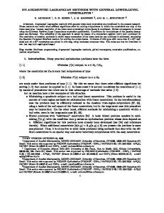
positive parameter called trust-region parameter, as it suggests how far from λ , model LCP can be accepted as an approximation of L . This is illustrated by Fig. 1: practically, a quadratic penalty term has been added to LCP to discourage choosing λ k far from λ .

B. Bundle methods for solving the Lagrangian dual Due to the problem formulation, the dual function L ( λ D , λ R ) is non-differentiable, however it is concave and its

α2

α1

sub-gradients with respect to the Lagrangian multipliers can be easily calculated: the t-th element of the sub-gradient vector g D (λ D ) with respect to λ D is g D t ( λ D ) = Dt −

åu

i ,t

åp

⋅ pi , t −

h, t

i∈I

å i∈I

å

rh ,t

(13)

h∈H

In the following, we simplify the notation by denoting λ = [ λ D , λ R ] , g(λ ) = éë g D ( λ D ) , g R ( λ R ) ùû and G = [ D, R ] . At iteration k of a Bundle method, the dual function has been evaluated at k multiplier vectors λ 0 K λ k −1 , and the corresponding values of the dual function, L(λ 0 )K L (λ k −1 ) , and of the subgradients, g(λ 0 )K g(λ k −1 ) , have been stored to form a bundle, denoted with β. The bundle is used to construct an upper approximation of L(λ ) , the cutting plane (CP) model

{

}

LkCP (λ ) = min L(λ j ) + g(λ j ) ⋅ (λ − λ j )' . j∈β

(14)

where the prime indicates transpose. This approximation is tight at least in every point λ j . Now, the idea would be to maximize the known function LCP instead of the unknown function L and to use resultant vector λ k as the next iterate. A major drawback of this approach is that LCP may be unbounded above, especially in the first iterations. Moreover,

LCP

will be a poor

approximation of L if λ k is “too far” from the points λ j . In order to overcome these drawbacks, we follow the so-called proximal Bundle method [26], namely a current point λ is selected (typically the one in the bundle that provides the greatest value of L), and the following quadratic problem is solved to find λ k 2ü 1 ì k λk − λ ý (15) max ív − k k k λ ,v 2 ⋅α î þ subject to

v k ≤ δ j + g(λ j ) ⋅ (λ k − λ )' where

∀j ∈ β

δ j = L ( λ j ) + g ( λ j ) ⋅ ( λ − λ j )' − L ( λ )

linearization error), ⋅

2

L

(12)

h∈H

ui ,t ⋅ ri ,t −

LCP λ

.

and the t-th element of the sub-gradient vector g R (λ R ) with respect to λ R is g R t ( λ R ) = Rt −

α3

(16) (known

λ3 − λ

λ1 − λ λ 2 − λ 1

2

3

Fig. 1. Impact of parameter α: λ , λ , λ represent the solutions of problem (15)-(16) for three different values of α (α1