Lagrangian Numerical Methods for Ocean

Lagrangian Numerical Methods for Ocean Biogeochemical Simulations

1

2

Francesco Paparella1,3 Marina Popolizio2

3

January 18, 2018

4

5

1

Division of Sciences and Mathematics New York University Abu Dhabi

2

Dipartimento di Matematica e Fisica Università del Salento Lecce

3

On leave from Dipartimento di Matematica e Fisica and I.N.F.N., Università del Salento Lecce.

6

7 8

9 10

11

Abstract

12

We propose two closely–related Lagrangian numerical methods for the simulation of physical processes involving advection, reaction and diffusion. The methods are intended to be used in settings where the flow is nearly incompressible and the Péclet numbers are so high that resolving all the scales of motion is unfeasible. This is commonplace in ocean flows. Our methods consist in augmenting the method of characteristics, which is suitable for advection–reaction problems, with couplings among nearby particles, producing fluxes that mimic diffusion, or unresolved small-scale transport. The methods conserve mass, obey the maximum principle, and allow to tune the strength of the diffusive terms down to zero, while avoiding unwanted numerical dissipation effects.

13 14 15 16 17 18 19 20 21 22

24

Keywords: Ocean biogeochemistry; lagrangian methods; advection reaction diffusion; unresolved flows.

25

1

23

26 27 28

Introduction

Biogeochemical problems in oceanography are usually expressed in terms of coupled advection-reaction-diffusion equations involving scalar fields, sometimes in large number, representing chemical species, biological species, or functional

1

29 30

groups (see, e.g., [1]). These fields are advected by the ocean currents, are subject to diffusion, and interact nonlinearly with each other. A generic, abstract form of oceanographical biogeochemical equations is the following ∂c1 + u · ∇c1 =D1 ∇2 c1 + f1 (c1 , . . . , cn ) ∂t .. . ∂cn + u · ∇cn =Dn ∇2 cn + fn (c1 , . . . , cn ) ∂t

31 32 33 34 35

36 37 38

where c1 , . . . , cn are the scalar fields, u is the water velocity field in the region of interest, which is assumed to be known, D1 , . . . , Dn are the diffusion coefficients, and the functions f1 , . . . , fn specify the local interactions among the scalar fields. The relative importance of the transport and diffusion terms is quantified by the Péclet numbers UL P el = Dl where U and L are, respectively, a characteristic speed and a characteristic length associated to the velocity field u. The relative importance of the transport and reaction terms is quantified by the Damköhler numbers Dal =

39 40 41 42 43 44 45 46 47 48 49 50 51 52 53 54 55 56 57 58 59

(1)

L U τl

where τl is a characteristic time scale associated with the reaction described by fl . The Damköhler number for phytoplankton may range from negligibly small up to O(10) [2]. While large values of the Damköhler number may amplify the patchiness of a reacting scalar as compared to a non–reacting one [3, 4] and make the problem stiff, the true source of numerical difficulties in biogeochemical applications lies in the enormous size of the Péclet number. If one takes the diffusivities to be the molecular ones (or computed from the mean square displacement of trajectories of individual plankton cells) then the Péclet numbers may easily exceed 1010 . Such a large value is reflected in the fact that ocean tracers (temperature, salinity, etc.) show structures from the scale of ocean basins down to submillimetric scales. Even accounting for a continuing rapid pace of improvement in computer technologies, it is quite obvious that, in the foreseeable future, no numerical code will be able to resolve such a wide interval of scales. In the absence of reaction terms, a reasonable way to deal with unresolved small scales is to parameterize the advective fluxes due to the unresolved scales with diffusion operators (often in a more complicated form than simple Laplacians). To this end there is an impressive array of techniques, ranging from explicitly adding new terms to the equations (e.g. in turbulence closures), to using flux or slope limiters (e.g. in finite volume methods), to advection and 2

60 61 62 63 64 65 66 67 68 69 70 71 72 73 74 75 76 77 78 79 80 81 82 83 84 85 86 87 88 89 90 91 92 93 94

95 96 97 98

interpolation (e.g. in semi-lagrangian methods) or dealiasing and filters (e.g. in pseudo–spectral methods). A review of numerical methods used for geophysical flows is given in [5]. In all these cases, however, the strength of the diffusive terms is determined not just by the physical parameters of the problem, but also by the size of the mesh. In fact, all these techniques may be viewed as different ways to average out the subgrid scales. Thus, in the presence of unresolved small scales, the values of the scalar fields at each grid node must be understood not as a pointwise evaluation of a function, but as an average over a spatial region having an extension comparable with the size of a computational mesh. Early studies already showed that changing the strength of the diffusive fluxes representing the unresolved scales may have a dramatic impact on the reaction terms [2, 6] and warned that a “mean field” approach might be inappropriate for modeling plankton dynamics. Later studies, conducted using realistic ocean models, showed strong fluctuations in plankton productivity depending on the advection scheme used and, most importantly, on the resolution [7, 8, 9]. The most recent assessment of the importance of the unresolved structures is found in [10]. As a first step to understand these results we need to observe that, for the full set of equations (1), one faces the overwhelming difficulty that an averaging operator does not commute with nonlinear reaction terms: fl (c1 , . . . , cn ) 6= fl (c1 , . . . , cn ). Because reactions terms are formally evaluated pointwise one would need to compute fl (c1 , . . . , cn ), but all that current grid–based codes can do is to compute fl (c1 , . . . , cn ). The wide chasm of unresolved scales means that the mesh-averaged values c1 , . . . , cn may be substantially different from their pointwise counterpart c1 , . . . , cn . As we shall see in the following, the bias produced by this effect may have either sign, depending, among other things, on the initial conditions. In the absence of any diffusive effect, that is, setting D1,...,n = 0 in (1), it is arguably better to avoid any discretization involving an Eulerian grid, and use a straightforward implementation of the method of characteristics. This leads to the following conceptually simple Lagrangian numerical scheme (for an overview on Lagrangian dynamics the interested reader is referred to [11, 12]): we uniformly seed the domain Ω with M particles, having position xi , i = 1, . . . , M , and then numerically solve  x˙ i = u(xi , t)     c˙1;i = f1 (c1;i , . . . , cn;i ) (2) ..   .    c˙n;i = fn (c1;i , . . . , cn;i ) with one among many viable ODE solvers. Here and in the following we use the shorthand notation cl;i = cl (xi , t) for the scalars sampled at the location of each particle (the notation is fully described in sec. 2). It is important to appreciate that, even when the number of particles is too small to fully sample 3

99 100 101 102 103 104 105 106 107 108 109 110 111 112 113 114 115 116 117 118 119 120 121 122

the small-scale structures present in the full solution of the PDEs, the values cl;i remain unaffected by the sparsity of the sampling, and are only affected by inaccuracies in the solution of the ODEs (2), due, e.g., to an imperfect knowledge of the velocity field u. This scheme is thus immune from the averaging problem discussed above. If, as is the case in oceanographic applications, the velocity field u is divergenceless, or nearly so, then an initially uniform sampling will remain uniform, or nearly so, at all future times. In this context the lack of a structured grid is just a nuisance: diagnostic and data analysis tasks may be performed after resampling the numerical solutions of (2) on a regular grid of choice, using, e.g., the methods discussed in [13, §5.3, p.128]. Unfortunately, the method of characteristics is not directly applicable to biogeochemical problems: the complete absence of diffusive effects in (2) would lead to paradoxical effects. For instance, if a water mass containing some phytoplankton but poor of nutrients were brought close to water masses devoid of phytoplankton but nutrient–rich, fluxes associated to small–scale motions would seed some plankton in the nutrient–rich water masses, leading, if the conditions are right, to a bloom. With the scheme (2) a particle full of phytoplankton could be brought arbitrarily close to a particle full of nutrients and yet there would be no exchanges between the two: the plankton would wither, and the nutrients would remain unused. In this paper we show how to augment the Lagrangian scheme (2) with couplings among nearby particles designed to mimic diffusive effects or, more generally, fluxes due to small-scale, unresolved transport processes. In order to be acceptable, such a coupling must possess the following three properties

123

1. respect mass conservation;

124

2. obey the maximum principle;

125

3. allow to recover the scheme (2) in the limit Dl → 0.

126 127 128 129 130 131 132 133 134 135 136 137 138 139 140 141

The importance of mass conservation is fairly obvious. Even for models using non–conserving reaction terms, there is no reason to introduce uncontrollable numerical sources and sinks of scalars. Schemes that do not obey the maximum principle may create maxima and minima unbounded by the maxima and minima of the initial conditions. In particular, scalar fields that should be non-negative (e.g. the concentration of a chemical species) may locally develop negative values, which, in turn, yield meaningless results with most reaction models. Being able to recover the scheme (2) means that one is free to tune the strength of the diffusive effects on the basis of modeling considerations alone, and not because of numerical requirements. We propose two distinct couplers that satisfy all these three properties. Of the two methods that we propose, the first is based on an integral formulation, the second is an heuristic recipe based on physical considerations. The two methods are distinct in the way used to enforce mass conservation. In both cases, however, the maximum principle is a direct consequence of the fact that the concentration of each particle after a diffusive step is determined as an average involving the concentrations of nearby

4

142 143 144 145 146 147 148 149 150 151 152 153 154 155 156 157 158 159 160 161 162 163 164 165 166 167 168 169 170 171 172 173 174 175 176 177 178 179 180 181 182 183 184 185 186 187

particles. Free parameters, appearing in both methods, can be used to tune the strength of the diffusive effects to extremely low values, or to zero, thereby maintaining the particles uncoupled. Particle–based methods are not a novelty. Smoothed particle hydrodynamics (SPH) has proved to be very suitable for highly compressible astrophysical problems, but flexible enough to be applied in many other settings [14], including heat conduction [15]. However, we felt that achieving all three of the above properties might be not straightforward with an SPH–inspired approach, therefore our methods are not based upon the differentiation of a smooth kernel. Other particle–based methods, closer to the spirit of the present work, have been proposed for diffusion and advection–diffusion equations [16, 17], but did not gain a large popularity. Few are the instances in which Lagrangian methods have been applied to geophysical problems. Nearly all numerical ocean models use grid–based methods, with the notable exception of the so–called “slippery sack” model [18]. This was initially a purely adiabatic, Lagrangian scheme, which was later augmented with a diffusive coupling between nearby particles [19]. More recently, embedding Lagrangian “blobs” within an Eulerian Ocean Circulation Model has been proposed as an effective way to parameterize sub–grid–scale processes [20], much in the same spirit as in the present work. The Lagrangian scheme (2) has been successfully applied to explain some incongruences between ecological models and observations [21]. When augmented with a diffusive coupling it has been used to explain the Fourier spectrum of a plankton concentration field [22]. We are not aware of other applications of Lagrangian schemes to ocean biogeochemistry. There exists more work on Lagrangian methods for modeling the atmosphere. In particular, a method based on contour advection and surgery has been highly successful in reproducing the observed distribution of stratospheric ozone [23, 24]. Lagrangian methods have shown to have advantages with respect to the Eulerian ones for simulating cloud microphysics [25]. They have also been profitably employed for studying atmospheric convection [26, 27]. For a recent survey on Lagrangian methods in atmospheric sciences see [28]. It is worth briefly mentioning that using stochastic processes for simulating diffusion in reaction–diffusion systems, albeit possible, is highly non–trivial. In the absence of reaction, adding a Brownian component to the deterministic trajectory of an advected particle is an effective way to simulate an advected– diffused passive scalar. But in the presence of reactions, random walkers must be coupled in some way (otherwise, once again, we’d fall in the paradox that arbitrarily close particles won’t affect each other’s concentrations). In a microscopic, stochastic description of diffusion and reaction the coupling is obtained by branching processes (see e.g. [29, §4.7 p.82] for an example applied to the FKPP equation). Unfortunately, devising the correct form of the branching process corresponding to a given set of reaction terms is a daunting task, in particular if one wishes to retain the freedom to tune the parameters or modify those terms. Thus our couplers are purely deterministic. They assume that particles, although being so small with respect to the size of the computational domain as to be considered punctiform, nevertheless encompass a large enough 5

188 189 190 191 192 193 194 195

mass of water to justify a deterministic description based on the notion of concentration of the scalars. The enormous potential of diffusively–coupled Lagrangian methods in biogeochemistry is illustrated by a simple example, inspired by the results obtained with a much more realistic model in [30]. In (1) we set n = 2 and choose a two–dimensional, incompressible velocity field u = (−ψy , ψx ) defined through the streamfunction ψ(x, y) = sin(x) sin(y) on the doubly–periodic domain (x, y) ∈ [0, 2π) × [0, 2π). The reaction terms are f1 (c1 , c2 ) = −r c1 c2 ,

196 197 198

199 200 201 202 203 204 205 206 207 208 209 210 211 212 213 214 215 216 217 218 219 220 221

222 223 224 225 226

f2 (c1 , c2 ) = +r c1 c2 ,

(3)

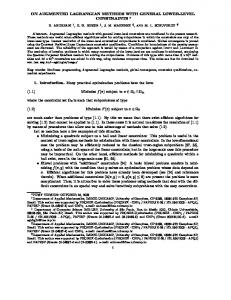
with r = 0.2. We may see the scalar field c2 as the spatial density of a consumer that grows at the expense of a resource whose density is c1 . The initial conditions are: c1 (x, y, 0) = cos2 (x/2), c2 (x, y, 0) = 10−4 . (4) We compute six solutions of this problem for progressively smaller diffusivities and correspondingly higher resolutions. The six meshes have 128 · 2k points in each direction, and the diffusivities are D1 = D2 = 10−3 · 2−2k , k = 0, . . . , 5. At each resolution, using substantially lower diffusivities would lead to severe oscillations and numerical instabilities. The solid lines in Figure 1A show the time evolution of the spatial average of c2 (that is, the mean consumer density). The dots show the same quantity computed by using the Lagrangian scheme (2), solved with the standard fourth–order Runge-Kutta integrator, augmented with one of the two diffusive couplers that will be presented in the following (namely, that of section 2.2). The six Lagrangian solutions all use just 1282 particles, and they differ only in the strength of the diffusive coupling. In this particular example, because of the quadratic nonlinearity, the same amount of resource c1 is consumed faster if it is spatially concentrated than if it is spread out on a larger surface but at lower concentrations. Thus smaller diffusivities, which better preserve the concentration peaks of the resource, yield a faster growth of the spatially averaged field c2 . In other words, they yield a higher productivity of the consumer. One might then be lead to hope that, just as unresolved turbulence can be usefully approximated by effective diffusion terms, in the same way effective reaction terms should be sought, representing the large–scale effects of the small– scale chemistry, with parameters tuned as a function of the resolution of the model. Here we give an example showing that this hope is unlikely to be fulfilled: we just change the initial conditions (4) with  x  y 4  x  y  c1 (x, y, 0) = sin sin , c2 (x, y, 0) = cos cos ,4 (5) 2 2 2 2 and repeat the same calculations described above. Because the resource and the consumer are now initially segregated into two nearly non–overlapping blobs, larger diffusivities bring in contact the resource and the consumer more quickly. As a result, we obtain the opposite effect as before: the growth of the spatially averaged consumer is fastest at the lowest resolution, and declines as the 6

0.4 0.3

0.28

128 256 512 1024 2048 4096

0.26

Average concentration

Average concentration

0.5

0.24 0.22 0.20

0.2

0.18

0.1 0.00

128 256 512 1024 2048 4096

20

40

Time

60

80

A

0.16 0.140

100

20

40

Time

60

80

B

100

Figure 1: Spatial average of the field c2 as a function of time. The solid lines are results obtained with a pseudo–spectral code, with progressively higher resolution and correspondingly lower diffusivity (see text). The dots are results obtained with a Lagrangian code using the coupler of sec. 2.2 with 1282 particles, where the strength of the diffusive coupling between particles is set as to match that of the pseudo–spectral computations. Panel A: calculations starting from the initial condition (4). Panel B: calculations starting from the initial condition (5).

227 228 229 230 231 232 233 234 235 236 237 238 239 240 241 242 243 244 245 246 247 248 249 250

resolution is increased (Figure 1B). Thus, hypothetical effective reaction terms intended to reproduce at low resolution the results obtained at highest resolution with the chemistry (3) should achieve the no small feat of adjusting the productivity that they yield not just to the resolution, but to the initial conditions, too. The diffusively–coupled Lagrangian scheme, having a diffusivity tunable independently of the resolution, is not affected by these problems, and reproduces fairly well with just 1282 particles the results of the pseudo–spectral code using the same strengths of the diffusive coupler as those used for Figure 1A. The four panels of Figure 2 show the field c2 at time t = 100 as computed by the pseudo–spectral scheme with 128 and 4096 grid points (panels A, B), and by the Lagrangian scheme (panels C, D) with diffusivities matching those of the pseudo–spectral calculations. The Lagrangian solutions are visualized by plotting partially overlapping colored squares centered at the particles’ positions, rather than by resampling the solution on a regular grid. This choice makes evident that the Lagrangian solution in panel D), reproduces the same range of fluctuations as the solution in the panel B), even though it obviously cannot resolve the fine structures created by the advective dynamics. The rest of the paper is organized as follows: in the following section we describe the diffusive couplers; in section 3 we compare the results obtained through our Lagrangian methods against known exact solutions or numerical solutions obtained with a pseudo–spectral code at much higher resolution; in section 4 we briefly discuss how to efficiently implement the methods; finally some concluding remarks are offered in section 5.

7

Figure 2: Field c2 at time t = 100. One quarter of the whole domain is shown. A) pseudo–spectral scheme on a 128 × 128 points grid. B) pseudo–spectral scheme on a 4096 × 4096 points grid. C) Lagrangian scheme with 1282 particles and a diffusion matching that of A). D) Lagrangian scheme with 1282 particles and a diffusion matching that of D). All cases use the initial conditions (5).

8

251

252 253 254 255 256 257 258 259 260 261 262 263 264 265 266 267 268

2

Diffusive couplers

We are not going to attempt a discretization of the Laplacian operator: evaluating the second derivatives of a field on a set of randomly distributed points and then devising a numerical scheme that satisfies mass conservation and the maximum principle would be quite challenging. Of the two methods that we propose, the first is the discrete counterpart of a convolution with the heat kernel; the second represents diffusive processes as exchanges of mass among nearby particles. Both methods have free parameters, which determine the strength of the diffusive effects. More precisely, they determine the rate at which the variance of a scalar field is dissipated. In section 3.1 we give an objective, quantitative way to attach an effective diffusivity to a given set of parameters. We feel that the first coupler has a more mathematically elegant formulation. However, it requires an iterative procedure to converge, which may make it slow. The second coupler is little more than a recipe to destroy variance, but its computational cost scales linearly with the number of particles. In order to make precise the notation that we shall use, let us recall that, given the smooth and bounded velocity field u which appears in equations (1), the system of ordinary differential equations x(t) ˙ = u(x(t), t)

269 270 271 272 273 274 275 276 277 278 279 280 281 282 283 284 285 286 287 288 289 290 291

(6)

defines a flow (e.g. [11, §2.1, p.18]) that links in a unique, smooth and invertible way the position a of a fluid particle at the initial time t0 to the position x(t; a) of the same particle at time t. By seeding the domain of interest with M particles initially at the positions ai , (i = 1, . . . , M ), and using the shorthand xi = x(t; ai ), and cl,i = cl (x(t; ai ), t), we may numerically solve the system of ordinary differential equations (2) in order to evaluate the solution at time t and positions xi of the equations (1), when the diffusivities D1 , . . . , Dn are all zero. The problem of introducing diffusive effects in this Lagrangian framework is greatly simplified if one takes a fractional step approach (e.g. [31, §17.1, p.377]). The reaction and advection terms are solved by integrating the ODEs (2) from time t to time t + τ , then a separate diffusive step, which solves the heat equation, is performed. During this diffusive substep the particles don’t move. Therefore, our methods for performing this step are more easily described in terms of the Eulerian coordinates xi of the particles, rather than in terms of their Lagrangian coordinates ai (which would be much harder). Even with this simplification, standard methods for solving the diffusion equation would be ill-suited for our purpose, because we cannot assume, in general, any regularity in the distribution of the particles. Here, for notational simplicity, we illustrate the methods for the case of a single scalar field c. Thus, we shall use the shorthands ci = c(xi , t) and ci (t + τ ) = c(xi , t + τ ). The generalization of the methods to the n scalar fields of the full PDEs (1) is straightforward.

9

292

293 294 295

2.1

First coupler

In place of a discretized form of the heat equation, we seek a discretized form of its solution; the latter, for a scalar field c, is given by the following convolution integral ˆ c(x, t + τ ) = k(x, y, τ )c(y, t) dy (7) Ω

296 297

298 299 300 301 302 303

where the kernel k is the fundamental solution of the heat equation in the domain Ω subject to the desired boundary conditions. In Rd the kernel is !  d2  2 kx − yk 1 exp − (8) k(x, y, τ ) = 4πDτ 4Dτ where D is the diffusion coefficient of the heat equation. Given M points x1 , . . . , xM in Ω, let Wij;τ be the elements of a matrix representing a discrete counterpart of the convolution (7) evaluated at the points xi , xj and across a time interval τ . By analogy with the properties of the kernel (8), we shall assume W to be a non–negative, symmetric matrix. The simplest discretization of the convolution (7) is given by ci (t + τ ) =

M X

Wij;τ cj

(9)

j=1 304

where we use the shorthands defined above. If M X

Wij;τ = 1,

(10)

j=1 305 306 307

that is, each column of W sums to 1, then the expression (9) is just a weighted average of all the concentration values {ci }. Therefore, it satisfies the maximum principle in the form: min {ci } ≤ ci (t + τ ) ≤

i=1,...,M 308

max {ci }.

i=1,...,M

(11)

If each row of W sums to 1, i.e. M X

Wij;τ = 1

(12)

i=1 309

then the expression (9) satisfies the conservation of mass in the form ! M M M M X X X X ci (t + τ ) = Wij;τ cj = cj . i=1

310 311 312

j=1

i=1

(13)

j=1

Thus, if the discrete kernel W is a doubly–stochastic matrix [32], i.e. it satisfies both (10) and (12), then the discrete model (9) obeys both the maximum principle and the conservation of mass. 10

313 314

315 316 317 318 319 320 321 322 323 324 325

Let us now describe how to construct such a discrete kernel W . Initially we define a crude discretization of the exact kernel (8) as follows   ( √ kx −x k2 , kxi − xj k < m 2Dτ exp − i4Dτj (14) Kij;τ = √ 0, kxi − xj k ≥ m 2Dτ where the nominal diffusivity D must be intended as a free parameter. The kernel K has a cut–off determined by m, also a free parameter, to avoid computing the negligible contribution of pairs of particles too far away from each other. Because K is not, in general, a doubly–stochastic matrix, we need to find a doubly–stochastic surrogate of K. The problem of rescaling a given matrix into a doubly–stochastic one is named balancing, and dates back to the 1930s. Since then, a large number of applications has been solved by resorting to the balance of matrices (see, e.g., [33] for a rich list of examples). We say that a matrix K can be balanced if there exist two diagonal matrices, diag(a) and diag(b), such that W = diag(a)K diag(b)

326 327 328

(15)

is doubly–stochastic. The fundamental theorem addressing this problem for non–negative matrices is due to Sinkhorn and Knopp [32]. Starting from any vector a0 with positive elements, they propose the following iteration:
−1 −1 bk+1 = K T ak ; ak+1 = (Kbk ) (16)

344

where the reciprocal is intended to be applied element–wise. Their theorem then states that the process converges to a doubly–stochastic matrix of the form (15) with a = limk→∞ ak , b = limk→∞ bk , if K has total support. A matrix K is said to have total support if every positive entry in K can be permuted into a positive diagonal with a column permutation. Under the conditions of the theorem the balancing is unique: K can be turned into one and only one doubly–stochastic matrix by means of multiplication by diagonal matrices (which are themselves unique up to a scalar factor). Our crude discretization of the Gaussian kernel, the matrix (14), has total support, because it is symmetric and has a positive main diagonal. Therefore, if Kij is a non–zero element, then the column permutation that swaps column i with column j brings to the main diagonal Kij , Kji , and no other element; the main diagonal thus remains positive. We can then define the discrete convolution kernel W that appears in (9) as the balancing of K. For our purposes it is important to note that K and W have the same pattern of zeros, therefore the particle pairs coupled by W are all and only those coupled by K.

345

2.2

329 330 331 332 333 334 335 336 337 338 339 340 341 342 343

346 347

Second coupler

A way to represent small-scale irreversible mixing processes is suggested by physical intuition, along the following heuristic argument, similar to those used 11

348 349 350 351 352 353 354

in [19, 22]. When two fluid particles happen to be close enough, they will exchange some portion of their mass, and, thus, of their advected scalars. Let qij ≥ 0 be the mass fraction exchanged between the i−th and the j−th particle, which are assumed to have the same mass. This fraction may be a function of the distance kxi − xj k and may be assumed to be zero when the distance exceeds some fixed threshold. Thus the concentration of the scalar c after a diffusion step at the position of the i−th particle will be ci (t + τ ) = ci −

M X

qij ci +

j=1 355 356 357

M X

(17)

where the first sum represents the losses to other particles, and the second sum represents the gains from other particles. The above expression can be re-arranged as     M M X X (18) ci (t + τ ) = 1 − qij  ci +  qij  ci j=1

358

qij cj

j=1

j=1

where the overline denotes the weighted average ci = 0≤

M X

PM

j=1 qij cj /

qij ≤ 1

PM

j=1 qij .

If

(19)

j=1 359 360 361 362 363

equation (18) shows that ci (t + τ ) is a linear interpolation between ci and ci , and therefore the maximum principle is satisfied. P P In addition, it is straightforward to verify that i ci , and i ci (t + τ ) = therefore the expression (17) conserves mass. As exchange fraction we shall use    √ kx −x k2 p  − i4Dτj , kxi − xj k < m 2Dτ d exp qij = (4πDτ ) 2 (20) √ 0, kx − x k ≥ m 2Dτ i

364 365 366 367 368 369 370 371 372 373 374 375

j

where p, D and m are free parameters and d is the dimensionality of the space. This particular choice is loosely suggested by the fact that if the scalar field carried by the i−th particle at time t were represented by a delta function, a diffusion process having diffusivity D, after a time τ would spread out the scalar with a resulting concentration proportional to  over the whole domain  2 exp − kxi − xj k /(4Dτ ) . The cut–off for large distances is also physically motivated: the small-scale, unresolved advective motions that this diffusion process is supposed to represent, cannot occur at an arbitrarily large speed; therefore, in a finite time τ only particles closer than some threshold length may exchange mass. Special care must be taken in choosing p small enough as to enforce the condition (19). A useful rule of thumb is: 1 p √ < , (4πDτ )d/2 N (m 2Dτ ) 12

(21)

377

where N (h) is the average number of particles that fall into a sphere of radius h.

378

2.3

376

379 380 381 382 383 384 385

Boundary conditions

So far we have discussed the diffusive couplers as if the computational domain were unbounded. When the domain is limited, any condition enforced along its boundaries is reflected in the kernel k appearing in the convolution solution (7), which ceases to be a simple Gaussian function. In the case of periodic boundary conditions, the kernel is an infinite sum of Gaussians, one for each of the periodic images. For example, on the segment [0, 2π) the kernel is ! 2 X (x − y + 2nπ) 1 √ . (22) exp − k(x, y, τ ) = 4Dτ 4πDτ n∈Z

386 387 388 389 390 391 392 393 394 395 396 397 398 399

400 401 402 403 404 405 406 407 408 409 410 411

√ If m 2Dτ < π, and we accept to approximate to zero the exponential when its argument is larger than or equal to m (as we do in (14) and in (20)), then only one term gives a non–zero contribution in the sum. This shows that the expressions (14) and (20) remain valid for periodic boundary conditions, provided that the norms kxi − xj k which appear in those expressions are considered as the minimum distance in the periodic domain between the particle i and the particle j. Another common boundary condition prescribes that the flux of tracers across any portion of the boundary has to be zero. When no particle is seeded outside of the domain, this condition is automatically enforced by both the diffusive couplers presented here. There is, however, a pitfall that needs to be brought to light. This is most easily illustrated in a one–dimensional domain. Let us consider the half–line [0, ∞). If we impose no–flux (a.k.a Neumann) boundary conditions at x = 0, then the heat kernel is " ! !# 2 2 1 (x − y) (x + y) k(x, y, τ ) = √ exp − + exp − . (23) 4Dτ 4Dτ 4πDτ This can be deduced by imposing an even symmetry to the initial condition which extends the problem to the whole line, and then restricting the solution back to the half–line. The even symmetry enforces the boundary condition. This implies that the points at x > 0 do exchange fluxes across the boundary with their mirror images at x < 0, but do so as to keep equal to zero the net flux at x = 0. If these virtual fluxes across the boundary are not taken into account, then, in proximity of the boundaries, the diffusivity of the scalar field is underestimated, even though the no–flux boundary condition is still correctly enforced. A solution to this problem might consist in using ghost particles strategically placed outside the domain so as to represent an even–symmetric field across it. In more than one dimension, this would be relatively straightforward only for straight boundaries, and would quickly escalate to a challenging problem for 13

423

boundaries of arbitrary shape. However, the √ contribution of the mirror images is important only within a distance of O( 2Dτ ) from the boundary. In high– Péclet number, under–resolved simulations, this distance would be comparable to or smaller than the inter–particle distance. We thus feel that attempting to fix this issue may not be worth the effort. In the following when we mention “no–flux boundary condition” we refer to the straightforward case in which no ghost particles are used. In the test cases we have not used the Dirichlet boundary condition. However we anticipate no difficulties in implementing this condition by distributing particles along the boundary and fixing their concentrations to a prescribed value. The same considerations about mirror images and ghost particles, subject to the appropriate symmetry, apply to this case as well.

424

3

425

3.1

412 413 414 415 416 417 418 419 420 421 422

426 427 428 429 430

431

432 433

Results Advection and diffusion

A first test for the diffusive couplers introduced in the previous section is to compare their performance for advection–diffusion problems in cases in which small–scale structures are progressively formed and eventually become under– resolved. An analytically–solvable, well–known, but non trivial test case is the following [34]: ∂c ∂c +y = D∇2 c (24) ∂t ∂x with initial condition c(x, y, 0) = cos(x). (25) In a domain vertically unbounded and horizontally periodic with period of 2π, the problem (24,25) has the exact solution c(x, y, t) = e

434 435 436 437 438

439 440 441 442 443

  3 −D t+ t3

cos (x − yt)

(26)

which develops arbitrarily high wavenumbers in the y−direction as times progresses due to the tipping over of the tracer streaks operated by the shearing flow (Figure 3). Multiplying (24) by c, averaging, and using (26) after an integration by parts, one finds the following explicit expression for the rate of dissipation of scalar variance     D E D
−2D t+ t33 d c2 2 − = D |∇c| = 1 + t2 e . (27) dt 2 2 Where the angular brackets denote a spatial average over one horizontal period and an arbitrary vertical length. In Figure 4 this expression is compared with the results obtained using the two couplers discussed in sec. 2. The numerical computations use the domain [0, 2π) × [−π, 3π], periodic in x and with no–flux boundary conditions in y. The

14

Figure 3: Numerical solution of (24,25) using the first coupler √ (§2.1). The parameters of the discretized kernel (14) are d = 2, m = 8, 2Dτ = π/512, τ = 0.1. The second coupler, with the parameters of Figure 4, produces visually indistinguishable results.

15

0.005

Coupler 1 Coupler 2 Exact Resolution-limited dissipation

2

0.003

d

−

dt




θ

2

0.004

0.002 0.001 0.000 0

50

100

Time

150

200

Figure 4: Rate of dissipation of scalar variance for the problem (24,25). Blue curve: results from the numerical simulation of Figure 3. Green curve:√ results using the second coupler (§2.2), with parameters p = 1.38·10−5 , m = 4, 2Dτ = π/256, τ = 0.1 for the exchange fraction (20). Red curve: expression (27) with D = 3.23 · 10−6 . Cyan curve: expression (27) with D = 10−3 ; the curve peaks off-scale at ≈ 0.0254. 444 445 446 447 448 449 450 451 452 453 454 455 456 457 458 459 460 461 462 463 464 465 466 467

number of particles is 128 × 256. The averages are computed in the central part of the domain, shown in Figure 3. The left–hand side of (27) is then computed from the particles’ concentrations. The value of the diffusivity D in the right– hand side of (27) is least–squares fitted to the numerical results. The fit extends from the beginning of the simulation up to the time of maximum dissipation. The value of the parameter p in the second coupler is tuned in order to match the fitted value of D = 3.23 . . . · 10−6 obtained with the first coupler with at least two significant digits. The match with the exact dissipation rate becomes inaccurate at later times, because when the stripes become under–resolved the tracer variance is aliased to lower wave numbers, and thus it is not damped as quickly as it should have been: obviously, an under–resolved computation does not perfectly reproduce the exact result. But the advantage of the Lagrangian approach should become clear by contrasting its results with those that could be attained by Eulerian methods. For example, with a pseudo–spectral code at a comparable resolution, the lowest diffusivity must be D ≈ 10−3 in order to avoid significant spurious oscillations. With that diffusivity one obtains the cyan curve in Figure 4: the dissipation rate peaks at time t ≈ 10 instead than t ≈ 70, by which time the streaks have all but disappeared. Thus, for a given resolution, when the diffusivity is as small as to make the computation under–resolved, with the Lagrangian approach we can obtain a dissipation curve that, albeit inaccurate, however peaks roughly at the right time and has roughly the correct dissipation strength; with pseudo–spectral or similar Eulerian methods we could obtain much more accurate shapes of the dissipation curves, but they would inevitably

16

Effective diffusion coefficient

10 -1 10 -2 10 -3

h = π8 h = 16π h = 32π h = 64π

10 -4 10 -5 10 -6 10 -7 -5 10

10 -4

10 -3

10 -2

Nominal diffusion coefficient

10 -1

Figure 5: Effective diffusivity D as a function of nominal diffusivity D for the first coupler (§2.1). Different symbols correspond to different values of the cut– off radius h. Different points with the same symbol correspond to different values of m. The nominal diffusivity is then given by (28). The black dashed line is the identity D = D.

468 469 470 471 472 473 474 475 476 477 478

correspond to diffusivity values determined by the resolution of the grid, which may be orders of magnitude larger than the physically relevant one. In fact, for each choice of the parameters, we can define the effective diffusivity of the method as the value D in the right-hand side of (27) that best fits the growing part of the numerical dissipation curve. This value, in general, does not coincide with the nominal diffusivity D, which appears in (14) and (20) and depends on the parameters as we shall discuss below. √Using the first coupler, in the discrete kernel (14) we set the cut–off radius m 2Dτ = h to be h = π/8, π/16, π/32, π/64. For each of these values we consider m = 3, 4, 6, 8, 12, 16. Fixing the value of the time step (we use τ = 0.1) the nominal diffusivity is then determined as D=

479 480 481 482 483 484 485 486 487 488 489

h2 . 2τ m2

(28)

Figure 5 shows the effective diffusivity as a function of the nominal diffusivity for the above values of h and m. Points that have the same h/m ratio yield nearly the same effective diffusivity. In other words, for fixed D, the effective diffusivity is fairly insensitive to the cut-off radius h, even when this is so small that only very few particles are involved: when h = π/64 only π particles, on average, fall within a disc of radius h. At high nominal diffusivities, the effective diffusivity nearly coincides with the nominal one: D(D) ≈ D. At low nominal diffusivities the effective diffusivity appears to be proportional to the square of the nominal one: D(D) ∝ D2 . Further tests suggest that the constant of proportionality scales as the square root of the particle density, and that the switch between the two regimes occurs 17

Effective diffusion coefficient

10 -2 10 -3 10 -4 10 -5

h = π8 h = 16π h = 32π h = 64π

10 -6 10 -7 10 -8 10 -5

10 -4

10 -3

10 -2

Nominal diffusion coefficient

10 -1

Figure 6: Effective diffusivity D as a function of nominal diffusivity D for the second coupler (§2.2). Symbols have the same meaning as in Figure 5. Blue markers refer to computations with p = 10−4 , red to p = 10−5 , green to p = 10−6 . The black dashed lines are the functions D = 10n D, with n = −5, −4, . . . , 0.

490 491 492 493 494 495 496 497 498 499 500 501 502 503 504 505 506 507 508 509 510 511

√ when the standard deviation 2Dτ of the discrete kernel (14) is of the same order of magnitude as the average distance between nearest particles. We did not further investigate the reasons of this change of slope and postpone an in-depth examination of the issue to a further work. Figure 6 shows the effective diffusivity obtained with the second coupler as a function of the coupler’s parameters appearing in the exchange fraction (20). The markers relative to h = π/64, m = 12, 16 are absent, because with those parameters the condition (19) does not hold: thus, the method violates mass conservation and blows up. The cut-off radius is determined as specified above for the first coupler, and the expression (28) for the nominal diffusivity still holds. As in that case, the effective diffusivity is fairly insensitive to the cut-off radius h when the ratio h/m is kept fixed. In contrast with the first coupler, the effective diffusivity appears to be roughly proportional to the nominal one across the whole range of diffusivities that we have tested. The effective diffusivity also appears to be roughly proportional to the parameter p. The effective diffusivity of the second coupler also depends on the density of the particles. If, keeping all other parameters the same, we double the average number of particles that fall within a disk of radius h, we find, from (17) and (20), that the average mass exchanged on a time step by each particle with its neighbors doubles. Thus the effective diffusivity is proportional to the particle density.

18

512

513 514 515 516 517 518 519 520 521 522

523 524 525 526 527 528 529 530 531 532 533 534 535 536 537 538 539 540 541 542 543 544 545 546 547 548 549 550 551 552 553 554

3.2

Reaction and diffusion

The methods described in the present work are designed for cases in which the Péclet numbers are extremely high. However, it cannot be excluded that some geophysical flows may, occasionally, be characterized by less extreme Péclet numbers. It is thus of interest to verify what may be the performance of the methods when the advection terms are not dominant over the diffusion ones. In the limit of zero Péclet numbers, the equations (1) reduce to reaction–diffusion equations. Even though we are not proposing our methods for this class of problems, we found informative to use one of them as a test case. Here we will consider the well-known Fisher–Kolmogorov–Petrovskii–Piskunov equation, namely ∂c = D∇2 c + c(1 − c). (29) ∂t For non-negative c, this equation describes the propagation of fronts joining a stable (c = 1) and an unstable (c = 0) region (e.g. [35] §13.2, √ p.439). There exist solutions with fronts propagating at any speed V ≥ 2 D. However, for a very large class of initial conditions, in particular those whose derivative √ has compact support, the propagation speed is the minimal one [36]: V = 2 D. When the function c assumes negative values the solution generally blows– up to minus infinity in a finite time. It is thus important to avoid numerical solution methods that generate spurious oscillations. In particular, this may be a problem when the diffusion √ coefficient is small, because the thickness of the front is also proportional to D. Thus, low diffusivities imply high gradients in the traveling front. We produce a numerical approximation of (29) by uniformly random seeding 1282 particles in the square [0, 2π] × [0, 2π]. We use no–flux boundary condition. Initially, all particles have a concentration of zero, except those having a coordinate x < 0.2, whose concentration is set to one. We then advance the solution with time steps of length τ = 0.1 by alternating one of the diffusive couplers of sec. 2 and the evaluation of the exact solution of the equation c˙ = c(1 − c). In Figure 7 we plot the propagation speed of the front as a function of the effective diffusivity of the method, evaluated as detailed in the previous subsection. The first coupler gives the best results, while the second coupler overestimates the speeds by about a factor 2.5. With both couplers the front propagation speed appears to be proportional to the square root of the diffusivity, as in the exact solution, except at very low diffusivities, where the front speed declines somewhat faster than the exact scaling. This excessive slow– down is in qualitative agreement with what was found in a stochastically forced version of equation (29). The primary effect of the random forcing was that of damping the leading tail of the propagating front, thus slowing it down [37]. We speculate that the random arrangement of the particles may play the role of the stochastic forcing. The front is well–resolved only at the lowest diffusivities. When D ≈ 10−3 the thickness of the front becomes comparable with the interparticle distance. Thus, most of the results of Figure 7 refer to runs in which the front is poorly

19

10 0

Front Speed

10 -1

h = π8 h = 16π h = 32π h = 48π

10 -2

10 -3 10 -7

10 -6

10 -5

10 -4

10 -3

10 -2

Effective diffusion coefficient

10 -1

Figure 7: Speed of propagation of the front in the solution of equation (29) as a function of the effective diffusivity. Symbols have the same meaning as in Figure 5. Blue markers refer to computations using the first coupler (sec.2.1) and the the green ones to computations using the second coupler (2.2) with p = 10−5 . √ The black dashed line is the theoretical speed V = 2 D.

555 556 557 558 559 560 561 562 563 564 565 566 567 568 569 570 571 572 573 574 575 576

resolved or not resolved at all. When the front is not resolved, the separation between the region where c = 1 and c = 0 appears as a jagged line, with meanders of characteristic size determined by the interparticle distance. We could not run this test case with a cut–off radius h = π/64, because this length results to be smaller than the percolation threshold: due to the random inhomogeneities in the distribution of the particles, after a short transient, no particle with concentration zero is found at a distance less than h from a particle with concentration higher than zero, thus the front stops propagating. In figure 7, we used h = π/48, instead. This elucidates the disadvantage of not having a velocity field stirring the particles: although Poissonian random gaps in the distribution of particles exist even in the presence of a stirring velocity field, they open and close as time progresses, rather than remaining static, and are thus far less damaging, as the results of the other tests should clearly illustrate. While we consider fitting the dissipation curve (27) as the best way to estimate the diffusivity of our proposed couplers when they are used for under– resolved flows at high Péclet number (that is, for their intended usage), it is nevertheless interesting to assess the performance of the couplers for approximating well–resolved diffusive processes. To this end, we seed the doubly–periodic domain [0, 2π)×[0, π/8) with 2500 particles, placed at uniformly random positions. We initially set the concentration of the i−th particle to ci = cos(kxi ), with integer k. We perform one step with each of the two couplers. For the coupler of section 2.1 we use h = π/8, m = 4.7, τ = 0.1; for the coupler of section 2.2 we

20

0.040

Exact BTCS Coupler 1 Coupler 2

0.035 0.030 0.025

Dk

0.020 0.015 0.010 0.005 0.000 0

20

40

60

Wavenumber

80

100

Figure 8: Diffusivity Dk (see eq. 30) for the exact solution of the heat equation (black horizontal line); for the BTCS finite difference discretization (red line); for the coupler of section 2.1 (blue squares); and for the coupler of section 2.2 (green circles). See text for parameters.

577

use h = π/16, m = 1, p = 10−3 , τ = 0.1. Then we compute σ(0) σ(τ ) k2 τ

log Dk = 578 579 580 581 582 583 584 585 586 587 588 589 590

591 592 593 594 595

(30)

where σ(0), σ(τ ) are, respectively the standard deviation of the concentration field at time t = 0 and t = τ . Using in the above expression the exact solution of the diffusion equation, ∂t c = D∇2 c, with initial condition c(x, 0) = cos(kx), one finds Dk = D for all k. However, for most numerical approximations of the heat equation Dk is a non–constant function of k. Figure 8 shows a comparison of the exact result, and of the approximations obtained by using our two couplers and one step of the BTCS (backward time, centered space) finite difference approximation with 200 equally–spaced nodes in [0, 2π), and a time step τ = 0.1. At low wavenumber, the above parameters are consistent with a diffusion coefficient D ≈ 0.035, although the random sampling of the domain produces a noticeable scatter between each wavenumber and the next. As a further test, we then use our couplers to produce numerical approximations of the solution of the following Turing instability problem [38]:        ∂ c1 1 −3 c1 D1 ∇2 c1 =q + . (31) c2 2 −5 c2 D2 ∇2 c2 ∂t A linear stability analysis of these equations is readily performed, and it shows that, with D1 = D2 /23 and D2 = 0.035, for q = 5 · 10−3 , only the wavenumber k = 1 is unstable, with a growth rate λ ≈ 0.0010 · · · ; for q = 5 · 10−2 , the wavenumbers k = 2, 3, 4 are unstable, and the fastest growing one is k = 3 with a growth rate λ ≈ 0.010 · · · ; for q = 5 · 10−1 , the wavenumbers k = 21

Standard deviation

A 10 2 10 1 10 0

10 -1 0 π/8 0

0

200

400

600

Time π

800

1000

1200

B 2π

C

π/8 0

0

π

2π

π

2π

D

π/8 0

0

Figure 9: Panel A: standard deviation of the numerical solution of equations (31) as a function of time; dashed lines refer to the coupler of section 2.1 and dotted lines to the coupler of section 2.2; solid lines are plotted for reference and have a slope corresponding to the growth rate of the maximally unstable wavenumber; red, green, blue lines refer, respectively, to q = 5 · 10−1 , 5 · 10−2 , 5 · 10−3 . Panel B: concentration field c1 at time t = 1000 in the calculation with q = 5 · 10−3 . Panel C: concentration field c1 at time t = 500 in the calculation with q = 5 · 10−2 . Panel D: concentration field c1 at time t = 100 in the calculation with q = 5 · 10−1 . The calculations of panels B, C, D refer to the coupler of section 2.2. For the other coupler the results are analogous.

22

609

5, . . . , 15 are unstable, and the fastest growing one is k = 10 with a growth rate λ ≈ 0.10 · · · . Perturbations along the y−direction are always damped when using these parameters in the domain of the previous test. The couplers use the same domain, number of particles and parameters as for the previous test, except that for the field c1 we set m = 17.5 when using the coupler of section 2.1, and p = 10−3 /23 when using the coupler of section 2.2. The initial concentrations of each particle are independently and randomly chosen with a Gaussian distribution with zero mean and unit variance. The results are summarized in Figure 9. In all cases Turing patterns emerge from the random initial conditions, and grow at a rate very close to that of the exact solution. The wavenumber that emerges is the correct one for q = 5 · 10−3 and for q = 5 · 10−2 . For q = 5 · 10−1 the pattern is a mixture of wavenumber k = 11 and k = 12. There are no appreciable differences neither in the patterns nor in the growth rate between the two couplers.

610

3.3

596 597 598 599 600 601 602 603 604 605 606 607 608

611

612 613 614 615 616

Advection, reaction and diffusion at different Damköhler numbers

We now return to the simple resource–consumer model (3) to test the performance of the Lagrangian couplers when the Damköhler number is changed. Here we do so by letting the reaction rate assume the values r = 0.04, 0.2, 1, 5, while keeping in all cases the same velocity field, which is defined by the following streamfunction ψ(x, y, t) = [(n mod 2) sin(x + φn ) − (1 − (n mod 2)) sin(y + φn )]

617 618 619 620 621 622 623 624 625 626 627 628 629 630 631 632 633 634 635 636

(32)

where n = btc (the largest integer smaller than t), “ mod ” denotes the remainder of the integer division, and φn is a uniformly random phase chosen in [0, 2π). This is an example of a “random renewing flow” (see e.g. [39] §11.1, p.320) which is very effective at mixing an advected scalar field. The characteristic spatial scale of this laminar flow is constant, but an advected field is subject to a continuous process of stretching and folding that produces a cascade of progressively smaller scales. Our benchmarks are numerical solutions of the problem (1) with the chemistry (3) and the velocity field induced by (32), solved on a uniform grid with 40962 nodes, on the doubly–periodic domain [0, 2π) × [0, 2π), with a Fourier– Galerkin pseudo–spectral code, and a diffusion coefficient D = 0.003/322 ≈ 2.9 · 10−6 . A slightly larger diffusivity was used than in the computations of Figure 1 at the same resolution, because at higher reaction rates the solution develops higher gradients in the concentration fields. We thus have tuned D so as to obtain a solution free of spurious oscillations at r = 5, and we have kept that value for all the reaction rates. We use both the uniform consumer initial condition (4) and the non overlapping blobs initial condition (5). Against the benchmark we compare the results obtained using the Lagrangian method with the couplers of section 2. For the first coupler we use a cut–off radius h = π/64 and m = 5.8. For the second coupler we use h = π/32, m = 4, 23

A

0.5

0.26

0.4

0.24 0.22

0.2

0.20

Mean

0.3

0.18

0.1 0.0 0 0.45

B

0.28

0.16 20

40

60

80

100

C

0.40

0.14 0

20

40

60

80

D

0.25

Standard Deviation

0.35

100

0.30 0.25

0.20

0.20 0.15

0.15

0.10 0.05 0.00 0

20

40

Time

60

80

100

0.10 0

r=0.04 r=0.2 r=1 r=5 20

40

Time

60

80

100

Figure 10: Mean (panels A,B) and standard deviation (panels C,D) of the consumer concentration field as a function of time using the chemistry (3) and the stirring field (32). Panels A,C refer to the initial conditions (4); panels B,D to the initial conditions (5). Different colors denote different reaction rates, as specified in the legend of panel D. Solid lines refer to results obtained with a pseudo–spectral code on a grid with 40962 nodes. Dotted and dashed lines refer to the Lagrangian method with 1282 particles and respectively, the coupler of section 2.1 and of section 2.2.

24

Figure 11: Consumer concentration field at time t = 50 for the numerical solutions of Figure 10 with r = 0.04 (panels A, B, C) and r = 5 (panels D, E, F), and initial conditions (5). Panels A, D are obtained with the pseudo–spectral code; panels B, E are obtained with the coupler of section 2.1; panels C, F are obtained with the coupler of section 2.2.

637 638 639 640 641 642 643 644 645 646 647 648 649 650 651 652 653 654 655 656 657

p = 10−5 . In both cases 1282 particles were used, the time step is τ = 0.1 and the ODEs (2) are solved with the standard fourth–order Runge–Kutta scheme. The results are summarized in Figure 10. Both Lagrangian methods reproduce very well the time evolution of the mean of the chemical fields, and reasonably well their standard deviation, even though the small–scale filaments produced by the stretching and folding dynamics of the flow are not resolved in the Lagrangian calculations. This is illustrated in Figure 11 which compares the consumer concentration field at time t = 50 for six of the numerical solutions summarized in Figure 10. Because the advecting flow is the same for all cases, solutions corresponding to the same reaction rate show the same large–scale pattern. Obviously, the delicate small–scale interleaving of filaments which is very well captured by the high–resolution pseudo–spectral calculations is missing in the low–resolution ones. The low–resolution computations severely undersample the filaments. However, owing to their Lagrangian nature, they do not produce any spurious mixing between nearby low– and high–concentration regions. Therefore they are able to reproduce almost exactly the same average and range of fluctuations observed in the fully–resolved, high–resolution calculations. Of course, the inability to resolve small scales inevitably produces undesirable side effects, so that a perfect match of the scalar statistics between resolved and unresolved calculations is impossible. In particular, if measured with the 25

670

criterion of section 3.1, the parameters used for the Lagrangian calculations yield an effective diffusivity slightly higher ( D ≈ 1.1 · 10−5 ) than the diffusivity of the pseudo–spectral code (the criterion suggests m ≈ 8 for the first coupler and m ≈ 7.5 for the second). When the effective diffusivity matches that of the pseudo–spectral code, in the later stages of the simulation the standard deviation remains too high and decays at a slower rate than in the pseudo–spectral benchmark. This occurs because, as stirring cascades the chemical tracers to unresolved small scales, the variance relative to those scales is aliased back to larger scales, where it is damped at an incorrect, lower rate. Using an ad-hoc higher effective diffusivity initially gives a slight underestimation of the standard deviation and, later on, a slight overestimation, while producing what we consider to be an acceptable approximation of a dynamics that requires a resolution 32 times higher to be fully resolved.

671

4

658 659 660 661 662 663 664 665 666 667 668 669

672 673 674 675 676 677 678 679 680 681 682 683 684 685 686 687 688 689 690 691 692 693 694 695 696 697 698 699 700

Implementation details

An efficient implementation of the diffusive couplers of section 2 requires a fast algorithm for finding all the particles falling within a distance h from any given particle. This fixed–radius near neighbors search is a classic problem in computational geometry. For arbitrary distribution of points, it can be solved by arranging the points in tree data structures such as quad–trees or Kd–trees (see e.g. [40] chap. 5, p.95). The use of trees leads to algorithms with a computational cost of O (M log(M )), where M is the number of points. When, as in our case, the particles are uniformly distributed, it is more convenient to use a lattice and hashing method, which has a computational cost of O(M ) [41]. The computational domain is overlaid with a regular lattice with square meshes of size h. To each mesh is assigned a unique index. For simplicity we use row–order indexing, although the Z–order indexing might improve cache efficiency. The particles are kept in a list, sorted according to the index of the mesh that contains each particle, which is easily computed from the particle’s position. The sorting is performed by means of the counting algorithm (e.g. [42] §8.2, p.194), which does not use pairwise comparisons, and has a complexity of O(M ). A hash table associates each mesh index with the first particle in the sorted list having that index. Thus, accessing all particles within the same mesh is an O(1) operation, because each mesh, on average, contains the same number of particles, due to their uniform distribution. To find all the particles within a distance h from a given one, one needs to compute the distance of the given particle from all the particles in the same mesh and in some of the adjacent meshes (three in 2D or four in 3D). After each time step, the particle list is sorted again, and the hash table is updated. If the size of the mesh h is decreased as the number of particles M increases in such a way as to maintain constant the average number of particles in each mesh, then the fixed–radius neighbor search problem is solved in O(M ) time. We did not attempt yet to produce a parallel version of our prototype code. However we don’t expect to face unusual difficulties or harsh performance penalties by pursuing a straightforward domain

26

713

partitioning strategy, in which each processor takes care of a contiguous block of meshes. In the case of the coupler of section 2.2, the computation of the exchange fraction (20) only increases the prefactor in the asymptotic scaling of the fixed– radius neighbor search. The overall algorithm is thus O(M ). In the case of the coupler of section 2.1, an analysis of the computational cost is more complicated, because it needs to take into account the cost of balancing the discrete kernel (14). The analysis of balancing algorithms is still an open problem, and we settled for the venerable Sinkhorn–Knopp algorithm only because it is extremely simple to implement. An assessment of the performances and of the relative merits of balancing algorithms, in particular on distributed– memory parallel architectures, is beyond the scope of this paper, and might become the subject of a future work.

714

5

701 702 703 704 705 706 707 708 709 710 711 712

715 716 717 718 719 720 721 722 723 724 725 726 727 728 729 730 731 732 733 734 735 736 737 738 739 740 741 742 743

Discussion and conclusions

In this paper we have investigated the viability of Lagrangian numerical methods to approximate the solution of advection–reaction–diffusion equations in cases where it is impossible to resolve all the scales of motion, as is commonplace for biogeochemical problems. The methods consist in alternating a purely Lagrangian step that solves the advection–reaction part of the equations with the method of characteristics, with a diffusive step that couples the particles moving along the characteristic lines of the advection–reaction problem. Two such couplers have been proposed. One amounts to a discrete version of the convolution with a Gaussian kernel, the other prescribes the exchanges between nearby particles of small portions of the mass carried by each. In both cases the resulting scheme conserves mass, respects the maximum principle and allows to tune the diffusivity down to zero, where the couplers have no effect, and the method of characteristics is recovered. We have carried several tests comparing the methods against exact solutions of advection–diffusion and reaction–diffusion problems, and against fully resolved numerical solutions of advection–reaction–diffusion problems obtained using a pseudo–spectral method run at significantly higher resolution than that of the Lagrangian code. In all cases the results have been fairly good, except in the case of the reaction–diffusion test, where the lack of an advection term that stirs the particles hampers the performance of the method. However, even in this unfavorable case, the methods are able to recover in a roughly correct way the main features of the solution and their scaling as a function of the diffusivity. Of course, when it is impossible to resolve all the spatial scales present in the solution, no method should be considered as completely satisfactory, and it is very likely that special cases could be found where it would perform far from well. For example, we don’t expect our Lagrangian method to perform brilliantly in reproducing the propagation of chemical fronts stirred by steady cellular flows. The speed of those fronts critically depends on an accurate description of the tails of the tracer distribution in proximity of the hyperbolic stagnation points at

27

781

the cell boundaries [43]. When the spatial structures are severely under resolved those tails are not reproducible, and the resulting speed is then unlikely to be correct. On the other hand, chemical fronts of that kind are not present in the oceans, and stagnation points, albeit present, are not steady; typical ocean mixing processes involve shearing, or stretching and folding dynamics, and in those cases our approach seems to be satisfactory. This paper does not suggest that our Lagrangian methods are competitive with, or even comparable to, a fully resolved numerical solution obtained with an Eulerian method, but rather that, by allowing to control the diffusivity independently of the resolution, the Lagrangian methods offer, when resolution can’t be further increased, a much better compromise than equally unresolved Eulerian methods. In this respect, diffusive couplers like those presented here could be seen more as a subgrid–scale parameterization of sorts, rather than as a discretization of a diffusion operator such as the Laplacian that appears in (1). While we believe that the present work is a successful proof–of–concept, some additional steps will be required in order to incorporate it into a realistic ocean circulation model. A first, necessary step is that of assessing the impact of interpolation schemes: here we conceded ourselves the luxury of using explicit expressions for the velocity fields and evaluate those at the position of each particle. A Lagrangian biogeochemistry module based on the schemes proposed here would need to acquire the velocity field from an Ocean Circulation Model. With probably the sole exception of the Lagrangian “Slippery Sacks” Model, this implies interpolating a velocity field known only on the nodes of an Eulerian grid. In addition, the current prototype implementation needs to be extended to three spatial dimensions and to distributed–memory parallel architectures. In the present form the couplers only represent homogeneous and isotropic diffusive processes. In ocean models, anisotropy is necessary, at least in the vertical direction, and the possibility to allow for spatially–dependent diffusivities is desirable. Finally, the existing Eulerian parameterizations for the sources and sinks of tracers, due to interactions with the bottom, with the air, and through river run–off must be adapted to the Lagrangian framework. These goals will probably be easier to achieve by modifying the coupler of section 2.2 where subgrid–scale fluxes are represented explicitly and locally as exchanges of mass between particles. They may be more demanding with the coupler of section 2.1, which requires the balancing of a matrix, a process that involves all particles simultaneously, even when the discretized kernel that couples them has a cut–off at a finite distance.

782

Acknowledgements

744 745 746 747 748 749 750 751 752 753 754 755 756 757 758 759 760 761 762 763 764 765 766 767 768 769 770 771 772 773 774 775 776 777 778 779 780

783 784 785 786

Part of this work was funded by Università del Salento through “Progetto 5xmille per la Ricerca”. We have benefited from discussions with Zouhair Lachkar, Olivier Paulis and Marcello Vichi. We are indebted to Clare Eayrs, Marina Levi and Shafer Smith who read and commented on earlier drafts of the paper.

28

787

788 789 790

791 792

793 794

795 796 797

798 799

800 801

802 803 804

805 806

807 808 809

810 811 812

813 814

815 816

817 818

819 820

821 822 823

References [1] Vichi, M., Pinardi, N., and S. Masina. “A generalized model of pelagic biogeochemistry for the global ocean ecosystem. Part I: theory.” Journal of Marine Systems, 64 (2007) 89–109. [2] Pasquero, C. "Differential eddy diffusion of biogeochemical tracers." Geophysical research letters, 32 (2005), L17603. [3] Mahadevan, A., and J. W. Campbell. "Biogeochemical patchiness at the sea surface." Geophysical Research Letters, 29 (2002), 32-1–32-4. [4] Richards, K. J., and S. J. Brentnall. "The impact of diffusion and stirring on the dynamics of interacting populations." Journal of theoretical biology, 238 (2006), 340–347. [5] Durran D. R. Numerical Methods for Fluid Dynamics: With Applications to Geophysics. Springer, 2nd edition, Berlin, 2010. [6] Brentnall, S. J., et al. "Plankton patchiness and its effect on larger-scale productivity." Journal of Plankton Research, 25 (2003), 121-140. [7] Lévy, M., A. Estublier, and G. Madec. "Choice of an advection scheme for biogeochemical models." Geophysical Research Letters, 28 (2001), 3725– 3728. [8] Lévy, M., et al. "Large-scale impacts of submesoscale dynamics on phytoplankton: Local and remote effects." Ocean Modelling, 43 (2012), 77–93. [9] Lévy, M., and A. P. Martin. "The influence of mesoscale and submesoscale heterogeneity on ocean biogeochemical reactions." Global Biogeochemical Cycles, 27 (2013), 1139–1150. [10] Martin, A. P., et al. "An observational assessment of the influence of mesoscale and submesoscale heterogeneity on ocean biogeochemical reactions." Global Biogeochemical Cycles, 29 (2015) 1421–1438. [11] Ottino, J. M. The kinematics of mixing: stretching, chaos and transport. Cambridge University Press (1989). [12] Samelson, R. M. and S. Wiggins. Lagrangian Transport in Geophysical Jets and Waves. Springer (2006). [13] Hockney, R. W., and J. W. Eastwood. Computer simulation using particles. Adam Hilger, Bristol, 1988. [14] Monaghan, J. J. "Smoothed particle hydrodynamics." Annual review of astronomy and astrophysics, 30 (1992), 543–574. [15] Cleary, P. W., and J. J. Monaghan. "Conduction modelling using smoothed particle hydrodynamics." Journal of Computational Physics, 148 (1999), 227–264. 29

824 825 826

827 828 829

830 831

832 833 834

835 836 837

838 839

840 841 842

843 844

845 846 847

848 849 850

851 852 853

854 855 856

857 858

859 860

[16] Degond, P., and S. Mas-Gallic. "The weighted particle method for convection-diffusion equations. I. The case of an isotropic viscosity." Mathematics of computation, 53 (1989) 485–507. [17] Degond, P., and F. J. Mustieles. "A deterministic approximation of diffusion equations using particles." SIAM Journal on Scientific and Statistical Computing, 11 (1990), 293–310. [18] Haertel, P. T., and D. A. Randall. "Could a pile of slippery sacks behave like an ocean?" Monthly weather review, 130 (2002): 2975–2988. [19] Haertel, P. T., L. Van Roekel, and T. G. Jensen. "Constructing an idealized model of the North Atlantic Ocean using slippery sacks." Ocean Modelling, 27 (2009), 143–159. [20] Bates M. L., S. M. Griffies, M. H. England. “A dynamic, embedded Lagrangian model for ocean climate models. Part I: Theory and implementation”. Ocean Modelling, 59–60 (2012) 41–59. [21] Koszalka, I., et al. "Plankton cycles disguised by turbulent advection." Theoretical population biology, 72 (2007), 1–6. [22] Bracco, Annalisa, Sophie Clayton, and Claudia Pasquero. "Horizontal advection, diffusion, and plankton spectra at the sea surface." Journal of Geophysical Research: Oceans, 114 (2009) C02001. [23] Edouard, S., et al. "The effect of small-scale inhomogeneities on ozone depletion in the Arctic." Nature, 384 (1996), 444–447. [24] Mariotti, A., et al. "The evolution of the ozone “collar” in the Antarctic lower stratosphere during early August 1994." Journal of the Atmospheric Sciences, 57 (2000) 402–414. [25] Hoffmann F., Y. Noh and S. Raasch. “The Route to Raindrop Formation in a Shallow Cumulus Cloud Simulated by a Lagrangian Cloud Model.” Journal of the Atmospheric Sciences, 74 (2017) 2125–2142. [26] Haertel, P., K. Straub and A. Fedorov. “Lagrangian overturning and the Madden– Julian Oscillation”. Quarterly Journal of the Royal Meteorological Society, 140 (2013) 1344–1361. [27] Haertel P., W. R. Boos, and K. Straub. “Origins of Moist Air in Global Lagrangian Simulations of the Madden–Julian Oscillation”. Atmosphere, 8 (2017) art.158. [28] Lin, J., et al. eds. Lagrangian modeling of the atmosphere. Geophysical Monograph Series Vol. 200. John Wiley & Sons, 2013. [29] Chorin A. J. and O. H. Hald. Stochastic Tools in Mathematics and Science. III ed. Texts in Applied Mathematics Vol. 58. Springer, 2013.

30

861 862

863 864 865

866 867

868 869

870 871 872

873 874

875 876

877 878 879

880 881

882 883

884 885 886

887 888 889

890 891

892 893 894

[30] Martin, A. P., et al. "Patchy productivity in the open ocean." Global Biogeochemical Cycles 16.2 (2002). [31] LeVeque, R. J. Finite volume methods for hyperbolic problems. Cambridge Texts in Applied Mathematics Vol. 31. Cambridge University Press, Cambridge (2002). [32] Sinkhorn, R., and P. Knopp. "Concerning nonnegative matrices and doubly stochastic matrices." Pacific Journal of Mathematics, 21 (1967) 343–348. [33] Knight, P. A., and D. Ruiz. "A fast algorithm for matrix balancing." IMA Journal of Numerical Analysis, 33 (2013), 1029–1047. [34] Rhines, P. B., and W. R. Young. "How rapidly is a passive scalar mixed within closed streamlines?." Journal of Fluid Mechanics, 133 (1983), 133– 145. [35] Murray J. D. (2007) Mathematical Biology I. An Introduction. Springer, Berlin, 3rd ed. [36] van Saarloos W. “Front propagation into unstable states”. Physics Reports 386 (2003), 29–222. [37] Doering C. R., Mueller C., and P. Smereka. “Interacting particles, the stochastic Fisher–Kolmogorov–Petrovsky–Piscounov equation, and duality.” Physica A 325 (2003) 243–259. [38] Turing A. M. “The chemical basis of morphogenesis”. Philosophical Transactions of the Royal Society of London B 237 (1952) 37–72. [39] Childress S. and A. D. Gilbert (1995) Stretch, Twist, Fold: The Fast Dynamo. Lecture Notes in Physics Monographs, Springer, Berlin. [40] de Berg, M., van Krefeld M., Overmars M., and O. Schwarzkopf (2008) Computational Geometry. Algorithms and Applications. Springer, Berlin, third edition. [41] Bentley J. L., Stanat D. F., and E. H. Williams Jr. “The complexity of finding fixed-radius near neighbors.” Information Processing Letters 6 (1977) 209-212. [42] Cormen, T. H., Leiserson C. E., Rivest R. L., and C. Stein (2009) Introduction to Algorithms. MIT press, Cambridge. [43] Tzella A. and J. Vanneste. “FKPP Fronts in Cellular Flows: The LargePéclet Regime.” SIAM Journal on Applied Mathematics 75 (2015) 1789– 1816.

31