Dec 10, 2005 - distribution for the case of rectangular correlation matrices. We il- .... The singular value decomposition (SVD) of this matrix answers the follow-.
arXiv:physics/0512090v1 [physics.data-an] 10 Dec 2005
Large dimension forecasting models and random singular value spectra Jean-Philippe Bouchaud1,2, Laurent Laloux1 M. Augusta Miceli3,1, Marc Potters1 February 2, 2008
1
Science & Finance, Capital Fund Management, 6 Bd Haussmann, 75009 Paris, France. 2 Service de Physique de l’Etat ´ Condens´e Orme des Merisiers – CEA Saclay, 91191 Gif sur Yvette Cedex, France 3 Universit` a La Sapienza, Piazzale Aldo Moro, 00185 Roma, Italy Abstract We present a general method to detect and extract from a finite time sample statistically meaningful correlations between input and output variables of large dimensionality. Our central result is derived from the theory of free random matrices, and gives an explicit expression for the interval where singular values are expected in the absence of any true correlations between the variables under study. Our result can be seen as the natural generalization of the Marˇcenko-Pastur distribution for the case of rectangular correlation matrices. We illustrate the interest of our method on a set of macroeconomic time series.
1
Introduction
Finding correlations between observables is at the heart of scientific methodology. Once correlations between “causes” and “effects” are empirically established, one can start devising theoretical models to understand the mechanisms underlying such correlations, and use these models for prediction 1
purposes. In many cases, the number of possible causes and of resulting effects are both large. For example, one can list an a priori large number of environmental factors possibly favoring the appearance of several symptoms or diseases, or of social/educational factors determining choices and tastes on different topics. A vivid example is provided by Amazon.com, where taste correlations between a huge number of different products (books, CDs, etc.) are sought for. In the context of gene expression networks, the number of input and output chemicals and proteins, described by their concentration, is very large. In an industrial setting, one can monitor a large number of characteristics of a device (engine, hardware, etc.) during the production phase and correlate these with the performances of the final product. In economics and finance, one aims at understanding the relation between a large number of possibly relevant factors, such as interest and exchange rates, industrial production, confidence index, etc. on, say, the evolution of inflation in different sectors of activity [1], or on the price of different stocks. Nowadays, the number of macroeconomic time series available to economists is huge (see below). This has lead Granger [2] and others to suggest that “large models” should be at the forefront of the econometrics agenda. The theoretical study of high dimensional factor models is indeed actively pursued [3, 4, 5, 6, 7, 1], in particular in relation with monetary policy [8, 1]. In the absence of information on the phenomenon under study, a brute force strategy would consist in listing a large number of possible explanatory variables and a large number of output variables, and systematically look for correlations between pairs, in the hope of finding some significant signal. In an econometric context, this is the point of view advocated long ago by Sims [9], who suggested to look at large Vector Autoregressive models, and let the system itself determine the number and the nature of the relevant variables. However, this procedure is rapidly affected by the “dimensionality curse”, also called the problem of sunspot variables in the economics literature [10]. Since the number of observations is always limited, it can happen that two totally unrelated phenomenon (such as, for example, stock prices and sunspots) appear to be correlated over a certain time interval T . More precisely, the correlation coefficient ρ, which would (presumably) be√zero if very long time series could be studied, is in fact of the order of 1/ T and can be accidentally large. When one tries to correlate systematically N input variables with M output variables, the number of pairs is NM. In the absence of any true correlation between these variables, the largest of these NM empirical correlation coefficients will be, for Gaussian variables, of order 2
q
ρmax ∼ 2 ln(NM)/T , which grows with NM. For example, ρmax ≈ 0.25 for N = M = 25 and T = 200. If the input and output variables are non Gaussian and have fat-tails, this number can be even larger: if two strongly fluctuating random variable accidentally take large values simultaneously, this will contribute a lot to the empirical correlation even though ρ should be zero for large T . In this paper we want to discuss how recent results in Random Matrix Theory [11, 12] allow one to alleviate this dimensionality curse and give a precise procedure to extract significant correlations between N input variables and M output variables, when the number of independent observations is T . The idea is to compare the singular value spectrum of the empirical rectangular M ×N correlation matrix with a benchmark, obtained by assuming no correlation at all between the variables. For T → ∞ at N, M fixed, all singular values should be zero, but this will not be true if T is finite. The singular value spectrum of this benchmark problem can in fact be computed exactly in the limit where N, M, T → ∞, when the ratios m = M/T and n = N/T fixed. As usual with Random Matrix problems [11, 12], the singular value spectrum develops sharp edges in the asymptotic limit which are to a large extent independent of the distribution of the elements of the matrices. Any singular value observed to be significantly outside these edges can therefore be deemed to carry some relevant information. A similar solution has been known for a long time for standard correlation matrices, for example the correlations of the N input variables between themselves that define an N × N symmetric matrix. In this case, the benchmark is known as the Wishart ensemble, and the relevant eigenvalue spectrum is given by the Marˇcenko-Pastur distribution [13, 14, 15]. Applications of this method to financial correlation matrices are relatively recent [16] but very active [17, 18]. Comparing the empirical eigenvalues to the correlation matrix to the theoretical upper edge of the Marˇcenko-Pastur spectrum allows one to extract statistically significant factors [16] (although some may also be buried below the band edge, see [17]). Similar ideas are starting to be discussed in the econometric community, in particular to deal with the problem of identifying the relevant factors in large dynamical factor models [19], and using them for prediction purposes (see also [6] for a different point of view). Here, we extend the Marˇcenko-Pastur result to general rectangular, non-equal time correlation matrices. We will first present a precise formulation of our central result, which we will then illustrate using an economically relevant data
3
set, and finally discuss some possible extensions of our work.
2
Mathematical formulation of the problem
We will consider N input factors, denoted as Xa , a = 1, ..., N and M output factors Yα , α = 1, ..., M. There is a total of T observations, where both Xat and Yαt , t = 1, ..., T are observed. We assume that all N + M time series are standardized, i.e., both X’s and Y ’s have zero mean and variance unity. The X and the Y ’s may be completely different, or be the same set of observables but observed at different times, as for example N = M and Yαt = Xat+1 . From the set of X’s and Y ’s one can form two correlations matrices, CX and CY , defined as: (CX )ab =
T 1X Xat Xbt T t=1
(CY )αβ =
T 1X Yαt Yβt . T t=1
(1)
In general, the X’s (and the Y ’s) have no reason to be independent of each other, and the correlation matrices CX and CY will contain information on their correlations. As alluded to above, one can diagonalize both these matrices; provided T > N, M – which we will assume in the following – all eigenvalues will, in generic cases, be strictly positive. In certain cases, some eigenvalues will however lie close to zero, much below the lower edge of the Marˇcenko-Pastur interval, corresponding to redundant variables which may need to be taken care of (see below). Disregarding this problem for the moment, we use the corresponding eigenvectors to define a set of uncorrelated, ˆ and output variables Yˆ . For example, unit variance input variables X X ˆ at = √ 1 X Vab Xbt , (2) T λa b where λa is the ath eigenvalue of CX and Vab the components of the correˆX ˆ T and C ˆ = Yˆ Yˆ T are sponding eigenvector. Now, by construction, CXˆ = X Y exactly identity matrices, of dimension, respectively, N and M. Using general ˆTX ˆ property of diagonalisation, this means that the T × T matrices DXˆ = X and DYˆ = Yˆ T Yˆ have exactly N (resp. M) eigenvalues equal to 1 and T − N (resp. T − M) equal to zero. ˆ Now, consider the M × N cross-correlation matrix G between the X’s and the Yˆ ’s: T X ˆ bt ≡ Yˆ X ˆT. Yˆαt X (3) (G)αb = t=1
4
The singular value decomposition (SVD) of this matrix answers the followˆ on ing question [20]: what is the (normalised) linear combination of X’s ˆ the one hand, and of Y ’s on the other hand, that have the strongest mutual correlation? In other words, what is the best pair of predictor and predicted variables, given the data? The largest singular value smax and its corresponding left and right eigenvectors answer precisely this question: the eigenvectors tell us how to construct these optimal linear combinations, and the associated singular value gives us the strength of the cross-correlation. One can now restrict both the input and output spaces to the N − 1 and M −1 dimensional sub-spaces orthogonal to the two eigenvectors, and repeat the operation. The list of singular values sa gives the prediction power, in decreasing order, of the corresponding linear combinations.
3
Singular values from free random matrix theory
How to get these singular values? If M < N, the trick is to consider the matrix M × M matrix GGT (or the N × N matrix GT G if M > N), which is symmetrical and has M positive eigenvalues, each of which being equal to the square of a singular value of G itself. The second observation is that the ˆTX ˆ Yˆ T are the same as those of the T × T non-zero eigenvalues of GGT = Yˆ X ˆTX ˆ Yˆ T Yˆ , obtained by swapping the position of Yˆ matrix D = DXˆ DYˆ = X ˆ and the Yˆ ’s are from first to last. In the benchmark situation where the X’s independent from each other, the two matrices DXˆ and DYˆ are mutually free [11] and one can use results on the product of free matrices to obtain the eigenvalue density from that of the two individual matrices, which are known. The general recipe [14, 11] is to construct first the so-called η−transform of the eigenvalue density ρ(u) of a given T × T non negative matrix A, defined as: Z 1 1 1 ηA (γ) = duρ(u) ≡ Tr . (4) 1 + γu T 1 + γA From the functional inverse of ηA , one now defines the Σ-transform of A as: ΣA (x) ≡ −
1 + x −1 η (1 + x). x A
(5)
Endowed with these definitions, one of the fundamental theorems of Free Matrix Theory [11] states that the Σ-transform of the product of two free 5
matrices A and B is equal to the product of the two Σ-transforms. [A similar, somewhat simpler, theorem exists for sums of free matrices, in terms of “Rtransforms”, see [11]]. Applying this theorem with A = DXˆ and B = DYˆ , one finds: ηA (γ) = 1−n+
n , 1+γ
n=
N ; T
ηB (γ) = 1−m+
m , 1+γ
m=
M . (6) T
From this, one easily obtains: ΣD (x) = ΣA (x)ΣB (x) =
(1 + x)2 . (x + n)(x + m)
(7)
Inverting back this relation allows one to derive the η−transform of D as: ηD (γ) =
q 1 1 − (µ + ν)γ + (µ − ν)2 γ 2 − 2(µ + ν + 2µν)γ + 1 2(1 + γ) �
�
(8) with µ = m − 1 and ν = n − 1. The limit γ → ∞ of this quantity gives the density of exactly zero eigenvalues, easily found to be equal to max(1 − n, 1 − m), meaning, as expected, that the number of non zero eigenvalues of D is min(N, M). Depending on the value of n + m compared to unity, the pole at γ = −1 corresponding to eigenvalues exactly equal to one has a zero weight (for n + m < 1) or a non zero weight equal to n + m − 1. One can re-write the above result in terms of the more common Stieltjes transform of D, S(z) ≡ η(−1/z)/z, which reads: q 1 SD (z) = z + (µ + ν) + (µ − ν)2 + 2(µ + ν + 2µν)z + z 2 . (9) 2z(z − 1) �
�
The density of eigenvalues ρD (z) is then obtained from the standard relation [11]: 1 1 1 ρD (z) = lim ℑ = lim ℑ [SD (z + iǫ)] , Tr ǫ→0 ǫ→0 π πT z + iǫ − D �
�
(10)
which leads to the rather simple final expression, which is the central result of this paper, for the density of singular values s of the original correlation ˆT: matrix G ≡ Yˆ X ρ(s) = max(1−n, 1−m)δ(s)+max(m+n−1, 0)δ(s−1)+
6
q
ℜ (s2 − γ− )(γ+ − s2 ) πs(1 − s2 )
(11)
,
0.8 m=0.4, n=0.2 m=n=0.3 m=0.7, n=1−m=0.3 m=n=0.8
ρ(s)
0.6
0.4
0.2
0
0
0.5 s
1
Figure 1: Continuous part of the theoretical random singular value spectrum ρ(s) for different values of n and m. Note that for n = m the spectrum extends down to s = 0, whereas for n + m → 1, the spectrum develops a (1 − s)−1/2 singularity, just before the appearance of a δ peak at s = 1 of weight n + m − 1.
7
where γ± are the two positive roots of the quadratic expression under the square root in Eq. (9) above, which read explicitely:1 q
γ± = n + m − 2mn ± 2 mn(1 − n)(1 − m).
(12)
This is our main technical result, illustrated in Fig. 1. One can check that in the limit T → ∞ at fixed N, M, all singular values collapse to zero, as they should since there is no true correlations between X and Y ; the allowed band in the limit n, m → 0 becomes: h√ √ √ √ i (13) s ∈ | m − n|, m + n . q
When n → m, the allowed band becomes s ∈ [0, 2 m(1 − m)] (plus a δ function at s = 1 when n + m > √ 1), while when m = 1, the whole band collapses to a δ function at s = 1 − n. When n + m → 1− , the inchoate δ-peak at s = 1 is announced as a singularity of ρ(s) diverging as (1 − s)−1/2 . Finally, when m → 0 at fixed√n, one finds that the whole band collapses again to a δ function at s = n. This last result can be checked directly in the case one has one output variable (M = 1) that one tries to correlate optimally with a set of N independent times series of length T . The result can q easily be shown to be a correlation of N/T . A plot of the SV density ρ(s) for values of m and n which will be used below is shown in Fig 2, together with a numerical determination of the SVD spectrum of two independent vector time series X and Y , after suitable diagonalisation of their empirical ˆ and Yˆ . correlation matrices to construct their normalised counterparts, X The agreement with our theoretical prediction is excellent. Note that one could have considered a different benchmark ensemble, where the independent vector time series X and Y are not diagonalized and ˆ and Yˆ before SVD. The direct SVD spectrum in that transformed into X case can also be computed as the Σ-convolution of two Marˇcenko-Pastur distributions with parameters m and n, respectively (noted MP 2 in Fig. 2). The result, derived in the Appendix, is noticeably different from the above prediction (see Fig. 1). This alternative benchmark ensemble is however not well suited for our purpose, because it mixes up the possibly non trivial correlation structure of the input variables and of the output variables themselves 1
One can check that γ+ ≤ 1 for all values of n, m < 1. The upper bound is reached only when n + m = 1, in which case the upper edge of the singular value band touches s = 1.
8
2
Theory (MP ) Theory (Standardized) Simulation (Random SVD)
ρ(s)
0.3
0.2
0.1
0
0
0.2
0.4
0.6
0.8
1
s
Figure 2:
Random Singular Value spectrum ρ(s) for m = 35/265 and n = 76/265. We show two possible theoretical calculations, corresponding either to bare random vectors X and Y , for which the singular value spectrum is related to the ‘square’ (in the free convolution sense) of the Marˇcenko-Pastur distribution ˆ and Yˆ , obtained after diagonalizing the empirical M P 2 , or standardized vectors X correlation matrices of X and Y . We also show the results of a numerical simulation of the standardized case with T = 2650.
9
1000 Gaussian X t−1Yt XtYt
P(ρ)
100
10
1 −0.75
−0.5
−0.25
0 ρ
0.25
0.5
0.75
Figure 3: Histogram of the pair correlation coefficient ρ between X’s and Y ’s, both at equal times and with one month lag. Note the ‘island’ of correlations around ≈ 0.6 for one-month lagged correlations, which corresponds to correlations between oil prices and energy related CPI’s one month later. We also show a Gaussian of variance 1/T , expected in the absence of any correlations. with the issue at stake here, namely the cross-correlations between input and output variables.
4
Application: inflation vs. economic indicators
We now turn to the analysis of a concrete example. We investigate how different groups of US inflation indexes can be explained using combinations of indicators belonging to different economic sectors. As “outputs” Y , we use 34 indicators of inflation, the monthly changes of the Composite Price Indexes (CPIs), concerning different sectors of activity including and excluding commodities. These indexes were not selected very carefully and some are very redundant, since the point of our study is to show how the proposed method 10
is able to select itself the relevant variables. As explanatory variables, “inputs” X, we use 76 different macroeconomic indicators from the following categories: industrial production, retail sales, new orders and inventory indexes of all available economic activity sectors, the most important consumer and producer confidence indexes, new payrolls and unemployment difference, interest rates (3 month, 2 and 10 years), G7 exchange rates against the Dollar and the WTI oil price itself. The total number of months in the period June 1983-July 2005 is 265. We want to see whether there is any significant correlation between changes of the CPIs and of the economic indexes, either simultaneous or one month ahead. We also investigated two-month lag correlations, for which we found very little signal. We first standardized the time series Y and X and form the rectangular correlation matrix between these two quantities, containing 34 × 76 numbers in the interval [−1, 1]. The distribution of these pair correlations is shown in ˆ ′ and for one-month lagged Yˆt X ˆ T correlaFig. 3, both for equal time Yˆt X t t−1 tions, and compared to a Gaussian distribution of variance T −1 . We see that the empirical distributions are significantly broader; in particular an ‘island’ of correlations around ≈ 0.6 appears for the one-month lagged correlations. These correspond to correlations between oil prices and energy related CPIs one month later. The question is whether there are other predictable modes in the system, in particular, are the correlations in the left and right flanks of the central peak meaningful or not? This question is a priori non trivial because the kurtosis of some of the variables is quite high, which is expected to ‘fatten’ the distribution of ρ compared to the Gaussian. Within the period of about thirty years covered by our time series, three major rare events happened: the Gulf War (1991-92), the Asian crisis (1998), and the Twin Towers Attack (2001). The kurtosis of the CPIs is the trace of the corresponding outliers, such as the food price index and its ‘negative’, the production price index excluding food, which are strongly sensitive to war events. Among economic indicators, the most responsive series to these events appear to be the inventory-sales ratio, the manufacturing new orders and the motor and motor parts industrial production indexes. In order to answer precisely the above question, we first turn to the analysis of the empirical self-correlation matrices CX and CY , which we diagonalize and represent the eigenvalues compared to the corresponding MarˇcenkoPastur distributions in Fig. 4, expected if the variables were independent (see the Appendix for more details). Since the both the input and output variables are in fact rather strongly correlated at equal times, it is not surpris11
ing to find that some large eigenvalues λ emerge from the Marˇcenko-Pastur noise band: for CX , the largest eigenvalue is ≈ 15, to be compared to the theoretical upper edge of the Marˇcenko-Pastur distribution 2.358, whereas for CY the largest eigenvalue is ≈ 6.2 to be compared with 1.858. But the most important point for our purpose is the rather large number of very small eigenvectors, much below the lower edge of the Marˇcenko-Pastur distribution (λmin = 0.215 for CX , see Fig. 4). These correspond to linear combinations of ˆ ˆ redundant (strongly √ correlated) indicators. Since the definition of X and Y include a factor 1/ λ (see Eq. (2)), the eigenvectors corresponding to these small eigenvalues have an artificially enhanced weight. One expects this to induce some extra noise in the system, as will indeed be clear below. Havˆ and ing constructed the set of strictly uncorrelated, unit variance input X ˆT. output Yˆ variables, we determine the singular value spectrum of G = Yˆ X If we keep all variables, this spectrum is in fact indistinguishable from pure ˆ precedes Yˆ by one month, and only one eigenvalue emerges noise when X ˆ and Yˆ are si(smax ≈ 0.87 instead of the theoretical value 0.806) when X multaneous. If we now remove redundant, noisy factors that correspond to, say, λ ≤ λmin/2 ≈ 0.1 both in CX and CY , we reduce the number of factors to 50 for ˆ and 16 for Yˆ 2 . The cumulative singular value spectrum of this cleaned X problem is shown in Fig. 5 and compared again to the corresponding random benchmark. In this case, both for the simultaneous and lagged cases, the top singular values smax ≈ 0.73 (resp. smax ≈ 0.81) are very clearly above the theoretical upper edge sue ≈ 0.642, indicating the presence of some true correlations. The top singular values smax rapidly sticks onto the theoretical edge as the lag increases. For the one-month lagged case, there might be a second meaningful singular value at s = 0.66. The structure of the corresponding eigenvectors allows one to construct a linear combination of economic indicators explaining a linear combinations of CPIs series. The combination of economic indicators corresponding to the top singular value evidences the main economic factors affecting inflation indicators: oil prices obviously correlated to energy production increases and electricity production decreases that explain the CPIs indexes including oil and energy. The second factor includes the next important elements of the economy: employment (new payrolls) affects directly the “core” indexes and the CPI indexes 2
The results we find are however weakly dependent on the choice of this lower cut-off, provided very small λ’s are removed.
12
ρ(λ)
30
20
10
0
0
2
4 λ
6
8
Figure 4: Eigenvalue spectrum of the N × N correlation matrix of the input variables CX , compared to the Marˇcenko-Pastur distribution with parameter n = 76/265. Clearly, the fit is very bad, meaning that the input variables are strongly correlated; the top eigenvalues λmax ≈ 15 is in fact not shown. Note the large number of very small eigenvectors corresponding to combinations of strongly correlated indicators, that are pure noise but have a small volatility. excluding oil. New economy production (high tech, media & communication) is actually a proxy for productivity increases, and therefore exhibits a negative correlation with the same core indexes. We have also computed the inverse participation ratio of all left and right eigenvectors with similar conclusions [16]: all eigenvectors have a participation ratio close to the informationless Porter-Thomas result, except those corresponding to singular values above the upper edge. Since Yt−1 may also contain some information to predict Yt , one could also study, in the spirit of general Vector Autoregressive Models [3, 5, 1], the case where we consider the full vector of observables Z of size 111, obtained ˆ by merging together X and Y . We again define the normalised vector Z, remove all redundant eigenvalues of Zˆ Zˆ ′ smaller than 0.1, and compute the T singular value spectrum of Zˆt Zˆt−1 . The size of this cleaned matrix is 62 × 62, 13
1
P(s’ 0, one introduces a second auxiliary variable Γ: √ Γ = f2 (z) − ∆, 17
(22)
to compute ρ2 (z): πρ2 (z) = −
Γ1/3 f1 (z) + . 24/3 31/2 z 22/3 31/2 Γ1/3 z
(23)
Finally, the density ρ(s) is given by: ρ(s) = 2sρ2 (s2 ).
(24)
References [1] for a review, see: J. H. Stock, and M. W. Watson, Implications of dynamical factor models for VAR analysis, working paper, June 2005. [2] C. W. J. Granger, Macroeconometrics, Past and Future, Journal of Econometrics, 100, 17 (2001). [3] J. Geweke The Dynamic Factor Analysis of Economic Time Series in D.J. Aigner and A.S. Goldberger eds. Latent Variables in Social Economic Models, North Holland: Amsterdam (1997). [4] J. H. Stock, M. W. Watson, Forecasting Inflation, Journal of Monetary Economics, 44, 293-335 (1999), Macroeconomic forecasting using diffusion indexes, Journal of Business and Economic Statistics, 20, 147-162 (2002), Forecasting using principal components from a large number of predictors, Journal of the American Statistical Association, 97, 1167-1179 (2002). [5] M. Forni, M. Hallin, M. Lippi and L. Reichlin, The Generalized Dynamic Factor Model: Identification and Estimation, The Review of Economic and Statistics, 82, 540-554 (2000); The Generalized Dynamic Factor Model: Consistency and Rates, Journal of Econometrics, 119, 231-255 (2004), The Generalized Dynamic Factor Model: One-Sided Estimation and Forecastings, mimeo (1999). [6] J. Bai, Inferential theory for factor models of large dimensions, Econometrica, 71, 135-171 (2003). [7] J. Bai, and S. Ng (2002) Determining the number of factors in approximate factor model, Econometrica, 70, 191-221 (2002). [8] B. Bernanke, J. Boivin, Monetary policy in a data rich environment, Journal of Monetary Economics, 50 525 (2003).
18
[9] C. A. Sims, Macroeconomics and Reality, Econometrica, 48, 1-48 (1980). [10] see, e.g. M. Woodford, Learning to believe in sunspots, Econometrica, 58, 277-307, (1990); see also M. Wyart, J.P. Bouchaud, Self referential behaviour, overreaction and conventions in financial markets, to appear in JEBO, (2005). [11] for a recent review, see: A. Tulino, S. Verd` u, Random Matrix Theory and Wireless Communications, Foundations and Trends in Communication and Information Theory, 1, 1-182 (2004). [12] A. Edelman, N. Raj Rao, Random Matrix Theory, Acta Numerica, 1-65 (2005). [13] V. A. Marˇcenko and L. A. Pastur, Distribution of eigenvalues for some sets of random matrices, Math. USSR-Sb, 1, 457-483 (1967). [14] J. W. Silverstein and Z. D. Bai, J On the empirical distribution of eigenvalues of a class of large dimensional random matrices, Journal of Multivariate Analysis, 54 175 (1995). [15] A. N. Sengupta and P. Mitra, Distributions of singular values for some random matrices, Phys. Rev. E 80, 3389 (1999). [16] L. Laloux, P. Cizeau, J.-P. Bouchaud and M. Potters, Noise dressing of financial correlation matrices, Phys. Rev. Lett. 83, 1467 (1999); L. Laloux, P. Cizeau, J.-P. Bouchaud and M. Potters, Random matrix theory and financial correlations, Int. J. Theor. Appl. Finance 3, 391 (2000): M. Potters, J.-P. Bouchaud and L. Laloux, Financial Applications of Random Matrix Theory: Old laces and new pieces, Acta Physica Polonica B, 36 2767 (2005). [17] Z. Burda, A. G¨ orlich, A. Jarosz and J. Jurkiewicz, Signal and Noise in Correlation Matrix, Physica A, 343, 295-310 (2004). [18] see the proceedings of the conference on Applications of Random Matrix Theory, published in Acta Physica Polonica B, 36 2603-2838 (2005). [19] G. Kapetanios, A new Method for Determining the Number of Factors in Factor Models with Large Datasets, mimeo Univ. of London (2004). [20] see, e.g., W. H. Press, B. P. Flannery, S. A. Teukolsky, W. T. Vetterling, Numerical Recipes in C : The Art of Scientific Computing, Cambridge University Press (1992).
19
[21] J. Baik, G. Ben Arous, and S. Peche, Phase transition of the largest eigenv alue for non-null complex sample covariance matrices, http://xxx.lanl.gov/abs/math.PR/0403022, to appear in Ann. Prob. [22] N. El Karoui, Recent results about the largest eigenvalue of random covariance matrices and statistical application, Acta Physica Polonica B, 36 2681 (2005).
20