Department of Computer Science and Engineering. Michigan State ... We then propose a dynamic Hamming distance range query algorithm ... To simplify notation in the rest of this paper, we use static problem and ...... Stated another way,.
Large Scale Hamming Distance Query Processing Alex X. Liu, Ke Shen, Eric Torng Department of Computer Science and Engineering Michigan State University East Lansing, MI 48824, U.S.A. {alexliu, shenke, torng}@cse.msu.edu
Abstract—Hamming distance has been widely used in many application domains, such as near-duplicate detection and pattern recognition. We study Hamming distance range query problems, where the goal is to find all strings in a database that are within a Hamming distance bound k from a query string. If k is fixed, we have a static Hamming distance range query problem. If k is part of the input, we have a dynamic Hamming distance range query problem. For the static problem, the prior art uses lots of memory due to its aggressive replication of the database. For the dynamic range query problem, as far as we know, there is no space and time efficient solution for arbitrary databases. In this paper, we first propose a static Hamming distance range query algorithm called HEngines , which addresses the space issue in prior art by dynamically expanding the query on the fly. We then propose a dynamic Hamming distance range query algorithm called HEngined , which addresses the limitation in prior art using a divide-and-conquer strategy. We implemented our algorithms and conducted side-by-side comparisons on large real-world and synthetic datasets. In our experiments, HEngines uses 4.65 times less space and processes queries 16% faster than the prior art, and HEngined processes queries 46 times faster than linear scan while using only 1.7 times more space.
I. I NTRODUCTION A. Background Given two equal length strings α and β, the Hamming distance between them, denoted HD(α, β), is the number of positions where the two strings differ. For example, HD(100, 111) = 2. Several classic similarity search problems are defined for Hamming distance. In particular, there is the Hamming distance range query problem, which was first posed by Minsky and Papert in 1969 [22], where the goal is to find all strings in a database that are within a Hamming distance bound k from a query string. A related problem is the K nearest neighbor (KNN) problem, where the goal is to find the K nearest neighbors in a given database with respect to Hamming distance to a given query string. Although these problems are extremely simple and natural problems, finding fast and space efficient algorithms for solving them remains a fundamental open problem where new results are still emerging. One reason these problems are widely studied is that they have meaning in a wide variety of domains such as nearduplicate detection, pattern recognition, virus detection, DNA sequence and protein analysis, error correction, and document classification. Hamming distance range query problems are especially useful in domains that deal with discrete data. For example, Manku et al. proposed a solution to the nearduplicate detection problem in Web crawling [19] that includes
978-1-4244-8960-2/11/$26.00 © 2011 IEEE
a new solution to the Hamming distance range query problem. The basic idea is to hash each document into a 64-bit binary string, called a fingerprint or a sketch, using the simhash algorithm in [11]. Simhash has the following property: if two documents are near-duplicates in terms of content, then the Hamming distance between their fingerprints will be small. Similarly, Miller et al. proposed a scheme for finding a song that includes a given audio clip [20], [21]. They proposed converting the audio clip to a binary string (and doing the same for all the songs in the given database) and then finding the nearest neighbors to the given binary string in the database to generate candidate songs. Similar applications have been used for image retrieval and iris recognition [15], [26]. B. Problem Statement In this paper, we focus on two variants of the Hamming distance range query problem. In a Hamming distance range query problem, we have a database T of binary strings, where the length of each string is m, and a query (α, k) where α is a binary string of length m and distance bound k is an integer that is at most m. The goal is to return the set of strings HD(T, α, k) = {β | β ∈ T and HD(α, β) 6 k}. Let n = |T |, the number of strings in T . We assume that T is fixed which means that we will process many distinct queries (α, k) with the given database T . We assume a solution preprocesses the database T in order to minimize the query processing time; that is, the time required to identify HD(T, α, k) for any query (α, k). We evaluate a solution to this problem using four criteria: its query processing time, the space it needs to store the preprocessed T , the time it needs to preprocess T , and the time it needs to update T when small changes to T are made. Our two variants of the problem differ in only one aspect. In the first variant, which we call the static Hamming distance range query problem, the Hamming distance bound k is fixed; that is, all queries will use the same value k and thus we can optimize the preprocessing of T for k. In the second variant, which we call the dynamic Hamming distance range query problem, the distance bound k is not fixed; that is, different queries may use different values of k and thus we cannot optimize the preprocessing of T for a particular k. Any solution to the dynamic bound problem is also a solution to the static bound problem, but the reverse is not true. To simplify notation in the rest of this paper, we use static problem and dynamic problem as shorthand for the two variants of the Hamming distance range query problem.
553
ICDE Conference 2011
C. Limitations of Prior Art For the static problem, most prior work focuses on the special case of k = 1. For arbitrary but small k, Manku’s algorithm in [19] represents the state-of-the-art. However, it uses an extensive amount of memory due to its aggressive replication of the database. In many applications, solutions for small k are all that is needed. For example, in the nearduplicate Web page detection system in [19], solutions for k = 3 are sufficient. For arbitrary but large k, two solutions have been proposed in [12], [13]; however, they are inefficient for problems with small k. For the dynamic problem, as far as we know, there is no space and time efficient solution for arbitrary databases. Existing solutions that use a trie [4], [5] are sensitive to the string length. However, in practice, long strings (e.g. 64-bits) are common. Other solutions assume that the strings in the database can be clustered and are therefore not suitable to databases with arbitrary strings [23]. D. Our Approach We focus on both the static and dynamic problems with arbitrary but small k red(i.e., k 6 10). For the static problem, we address the space issue in prior art by dynamically expanding the query on the fly. This “query expansion” greatly reduces the number of database replicas needed. We use Bloom filters to quickly identify and eliminate most unsuccessful queries. The end result is that we not only save space but also achieve faster query processing than prior art. We use HEngines (s standing for “static”) to denote our algorithm for the static problem. For the dynamic problem, we address the string length issue in prior art using a divide-and-conquer strategy. For a given Hamming distance range query instance, if the distance bound k exceeds a given threshold, we divide the query string in half, all the strings in T in half, and k in half and then recursively solve the resulting smaller Hamming distance query instances. Thus, our algorithm’s query processing time grows with the logarithm of string length. We use HEngined (d standing for “dynamic”) to denote our dynamic Hamming distance range query algorithm. Most modern microprocessors such as current 64-bit x86 processors have a popcount(s) instruction that returns the number of ones in a bit string s. Thus, the hamming distance between two bit strings α and β of length no more than 64 can be calculated by only two instructions: s = α ⊕ β and HD(α, β) =popcount(s). Thus, our query processing time roughly grows as a function of m/64. For moderate m, we can assume query processing time is independent of m. E. Summary of Experimental Results We implemented our HEngine algorithms in Java 1.6. To perform a side-by-side comparison, we also implemented Manku’s algorithm in Java 1.6. We evaluated them using a large real-world dataset as our database T and randomly generated queries. In our experiments, HEngines uses 4.65 times less memory and is 16% faster in query processing, 4.15
times faster in preprocessing, and 4.53 times faster in handling data updates. We also perform an ‘unfair” comparison of HEngined with Manku’s algorithm; the comparison is unfair because Manku’s algorithm cannot handle dynamic Hamming distance range queries. In our experiments, HEngined uses 6.12 times less memory and is 50.7% slower in query processing, 13.35 times slower in preprocessing, and 2.28 times faster in handling data updates. More preprocessing and query processing time is the price that HEngined pays for its flexibility in handling varying k. In our experiments, HEngined processes queries 46.42 times faster than linear scan using only 1.7 times more space. F. Key Contributions We make three key contributions. First, we propose an algorithm for the static problem that uses less memory but processes queries more quickly than prior art. redSecond, we propose an efficient algorithm for the dynamic problem that works with long strings (e.g. 64-bits). Last, we implemented our algorithms and conducted extensive experiments on both real and synthetic datasets. The rest of this paper proceeds as follows. We first discuss related work in Section II. Then, we present HEngines and HEngined in Sections III and IV, respectively. We report our experimental results in Section V. We conclude the paper in Section VI. II. R ELATED W ORK In this section, we first discuss prior work on the static and dynamic problems. Then, we review prior work that converts similarity search problems in other distance metrics to similarity search problems in Hamming space. A. Static Hamming Distance Range Query We classify prior work on the static problem into three categories based on bound k: (a) k = 1, (b) k is small but k > 1, (c) k is large. k = 1: Yao and Yao proposed an algorithm with O(m log log n) query time and O(nm log m) space [27]. Yao’s algorithm first cuts the query string and each string in the database in half, and then it finds exact matches in the database for the left and right halves of the query string; for each match, Yao’s algorithm recursively applies this cutting strategy until the query string is just 1 bit. This recursive cutting is the fundamental strategy used in several subsequent algorithms for the static problem including ours, although Yao and Yao only focused on the k = 1 case. In [9], Brodal and Ga¸sieniec proposed a trie-based solution with O(m) query time and O(nm) space. Brodal and Venkatesh proposed an algorithm with O(1) query time (assuming that m fits within one memory word) and O(mn log m) space that finds a string in the database that differs by at most 1 from the query string using perfect hash functions [10]. Unfortunately, we cannot leverage this algorithm in our work because we need to find all strings in the database that differ by at most 1 from the query string.
554
k is small but k > 1: This problem was mainly investigated in Manku et al.’s seminal work [19]. Manku et al. proposed an algorithm for small k (up to 7) using a cluster of machines. They generalized Yao’s algorithm by cutting database strings and the query string into k + 1 segments (k > 2). This method is based on the observation that if two string are within Hamming distance k, then at least one of the k + 1 segments are exact matches for the two strings. This algorithm achieves high throughput for large databases. Its main drawback is high memory consumption due to extensive replication of the database. This algorithm needs to replicate the database k + 1 times and for each copy, sort the strings based on one of the k + 1 segments. This limits the scalability of the approach for large databases or large k. For this reason, Manku et al. developed a distributed implementation where tables are stored on a farm of machines. Our algorithm generalizes Yao’s and Manku’s algorithm in the following way. Their algorithms reduce to exact matching algorithms in the base case. Our algorithm reduces to an approximate matching algorithm in the base case (i.e., two segments are within a certain Hamming distance z). This generalization gives us more flexibility to trade query time for storage space. As z increases, our algorithm uses less space but requires more query time. This adaptability allows our algorithm to be used for applications with varying space and query time requirements. In our experiments, our algorithm HEngines for the static problem with z = 1 uses 4.65 times less memory than Manku’s algorithm while being 16% faster. k is large: Two solutions have been proposed in [12], [13]; however, both are inefficient for problems where k is small. B. Dynamic Hamming Distance Range Query In the theory community, Arslan and Eˇgecioˇglu proposed a simple solution using tries [5]. Its query processing complexity is O(mk+2 ) and its space complexity is given by the space occupation of the trie plus additional space to store O(mk+1 ) trie nodes. Later, Arslan proposed another trie-based algorithm with query processing complexity O(m(log 4/3 n − 1)k (log2 n)k+1 ) [4]. No experimental results were given in [5] and [4]. Because the trie processes the query string bit-by-bit, the query processing time of the trie approach is sensitive to string length m. In contrast, the query processing time of our dynamic Hamming distance range query algorithm HEngined grows with the logarithm of string length assuming that all strings fit within a memory word. In the database community, Qian et al. proposed a solution using a dynamic indexing technique called ND-tree [23]. They cluster the database and build the tree from the clusters. A Hamming distance range query is processed from the root node pruning away any nodes that are out of the query bound until we find the leaf nodes containing the desired data. This algorithm’s performance depends on whether the database strings can be well clustered. In contrast, our algorithm for the dynamic problem HEngined works reasonably well even on synthetic randomly generated data sets.
C. Set Similarity Join Problem Similarity join is a common problem in near-duplicate detection and document clustering [3], [7], [16], [25]. It is a generalization of the well-known nearest neighbor problem. Two sets are joined to form all pairs of objects whose similarity score is above a threshold. When the two sets are identical, it is a self-join problem. The similarity join problem differs from Hamming distance range queries in that the focus in similarity joins is to find all the similar pairs from two given sets. In Hamming distance range queries, the focus is to preprocess the database that is repeatedly queried. Thus, for Hamming distance range queries, preprocessing time is relatively unimportant whereas query time is important. For similarity join, there is no separation of preprocessing time and query time. In [3], Arasu et al. proposed a similarity join algorithm called PartEnum, which is in essence a non-recursive version of Manku’s algorithm. In our experiments, our static problem algorithm HEngines outperforms PartEnum. III. S TATIC H AMMING D ISTANCE R ANGE Q UERIES In this section, we present our static problem algorithm HEngines. Because k is fixed, we refer to the query as just the string α. We first present the theoretical foundation of HEngines. Second, we describe how HEngines preprocesses the database and processes queries. Third, we discuss a recursive implementation of HEngines as well as how to efficiently update the database when small changes to T are made. Then, we describe how we improve query processing time using Bloom filters. Further, we give the space and time analysis of HEngines . We show that theoretically HEngines requires significantly less memory space and less preprocessing time than the prior art. A. Overview of HEngines Algorithm There are three straightforward solutions for solving the static problem: linear scan, query expansion, and table expansion. Linear scan uses little space but query processing is slow. Table expansion uses a lot of space but query processing is fast. Query expansion uses the same amount of space as linear scan and can be much faster than linear scan depending on the values of k, m, and n, but it is much slower than table expansion. With linear scan, each string in T is compared to the query string α to find all strings that are within Hamming distance k of α. This requires a total of n string comparisons. Query expansion computes all strings that are within Hamming distance k of the query string α (including α itself). P For any� binary string α of length m, there are a total of kb=0 m b strings that are within Hamming distance k of α, denoted α1 , · · · , αPk (m) . Query expansion generates all of these b=0 b strings and does an exact match search within T for each of these strings. Since we are doing an exact match search, we can use binary � assuming we sort T first. This requires Pk search, a total of b=0 m b log n string comparisons, which can be much fewer than n. Table expansion requires a preprocessing step. For each binary string β in T , one first precomputes all the strings whose Hamming distance from β is less than or
555
equal to k (including β P itself). For � any binary string β of length k m, there are a total of b=0 m b strings that are within Hamming distance k, denoted δ1 , · · · , δPk (m) . Preprocessing b=0 b concludes by storing the pairs (δ1 , β), · · · , (δPk (m) , β) in a
finding all strings β in T that satisfy the signature match property of Theorem 3.2 and then verify which of these strings actually are within Hamming distance k of α.
new database denoted as T in sorted order. Query processing involves finding all pairs of strings in T k whose first string is α and returning the second string of each such pair. Because T k is sorted, these strings will appear in consecutive locationsP and the � entire range can be efficiently found in k O(log n( b=0 m b )) string comparisons using binary search. s HEngine balances storage space and processing time by carefully expanding the database so that a Hamming distance query can be processed by an efficient combination of selected query expansion and linear scans. The theoretical foundation of HEngines is captured in the following results. To formally state these results, we define the following notation. Definition 3.1: For a length m string β, we define r-cut(β) to be the process of splitting β into r substrings (β1 , . . . , βr ) where the first r − (m mod r) substrings have length ⌊m/r⌋ and the last m mod r substrings have length ⌈m/r⌉. We overload notation and use r-cut(β) to also denote (β1 , . . . , βr ). Theorem 3.1: For any two binary strings β and γ such that HD(β, γ) 6 k, consider r-cut(β) and r-cut(γ) where r > ⌊k/2⌋+ 1. It must be the case that HD(βi , γi ) 6 1 for at least q = r − ⌊k/2⌋ different values of i. Proof: We prove the theorem by showing that HD(βi , γi ) > 2 for at most ⌊k/2⌋ different values of i. Observe that ⌊k/2⌋ + 1 > k/2 + 1/2; equality holds when k is odd. Suppose HD(βi , γi ) > 2 for ⌊k/2⌋ + 1 values of i. This would imply HD(β, γ) > 2( k2 + 21 ) > k + 1 > k contradicting the fact that HD(β, γ) 6 k. Thus the result follows. Theorem 3.1 implies that all β with HD(α, β) 6 k must satisfy a signature match property that is formally expressed in Theorem 3.2. Definition 3.2: For any length m string β and r > ⌊k/2⌋ + 1, a signature of β, denoted β-signature, is any choice of q = r − ⌊k/2⌋ substrings from r-cut(β). We define the choice vector of β-signature as (i1 , i2 , . . . , iq ) where 1 6 i1 < i2 · · · < iq 6 r represents the q substrings chosen from r-cut(β). � Any string β has rq signatures. Definition 3.3: For any two length m strings α and β and r > ⌊k/2⌋ + 1, we say that two signatures α-signature and β-signature are compatible if their choice vectors are identical. We say that compatible signatures α-signature and β-signature match if HD(αij , βij ) 6 1 for 1 6 j 6 q. That is, each of the q substrings from α-signature is within Hamming distance 1 of the corresponding substring from β-signature. Theorem 3.2: Consider any string β ∈ T such that HD(α, β) 6 k. Given any r > ⌊k/2⌋ + 1, it follows that at least one signature β-signature matches its compatible signature α-signature. The basic idea of HEngines is to preprocess T to facilitate
We preprocess a database T given Hamming distance bound k �and segmentation factor r > ⌊k/2⌋ + 1 by constructing r q duplicates of T , one for each signature. We call this set of tables the signature set of T for distance bound k and segmentation factor r; we call each table in the signature set a signature table. We begin by computing r-cut(β) for all β ∈ T . In each signature table, each string β is permuted so that the q chosen substrings are moved to the front of the string. In each permuted string, the original order among the q chosen substrings is maintained. Likewise, the original order among the r − q other substrings is also maintained. Finally, we sort the permuted strings in each table to enable efficient binary searches. The pseudocode of the above signature set construction procedure (the preprocessing phase of HEngines) is shown in Algorithm 1. We use B(i) to denote the i-th element in set B and a|b to denote the concatenation of substrings a and b.
k
b=0
b
B. HEngines Preprocessing
Algorithm 1: HEngines preprocessing algorithm Input: (1) Database T in which the length of each string is m. (2) Hamming distance bound k. (3) Segmentation factor r. Output: The signature set of T based on distance bound k and segmentation factor r. 1 2 3 4 5 6 7 8 9 10 11 12
13 14 15 16 17 18 19 20 21 22 23 24 25
Function build (T , k, r) begin RS := ∅; � for i := 1 to rq do Ti := ∅; foreach β ∈ T do PS = permute (β, � k, r); for i := 1 to rq do insert PS (i) into Ti ; for i := 1 to
� r r−⌊ k ⌋ 2
do
insert Ti into RS; return RS;
Function permute (β, k, r) begin PS := ∅; Compute r-cut(β). � for i := 1 to rq do IS :=nextChoice (r, q); front := “”; back := “”; foreach x ∈ IS do front := front|βx ; foreach y ∈ [1, r] − IS do back := back|B(y); insert front|back into PS; return PS;
We illustrate the HEngines preprocessing in Fig. 1. Here we have m = 64, k = 4, r = 3 and q = 1. The lengths of the� three substrings will be 21, 21, and 22. We construct the r q = 3 tables by moving q = 1 different substrings to the left in each table. These 3 tables constitute the signature set of T based on distance bound 4 and segmentation factor 3.
556
5! $!%!&
$"
$#
$!%"&
$"
$#
$!%""&
$"
$#
$"%!&
$!
$#
$"%"&
$!
$#
Algorithm 2: HEngines query processing algorithm Input: (1) Query string α of m bits. (2) The signature set S of T based on distance bound k and segmentation factor r. Output: All the binary strings in T that are within Hamming distance k from α.
!
$!
5"
!
"
#
$"%""& $!
23.343-),5
#
3 4
$!
$#
$!
$"
$#%"&
$!
$"
$#%"#& $!
$"
$"
$#
5 6 7
$# $#%!&
$!
'()*+,-.*/01,$
$#
5#
1
$#
2
$"
"
$"
$!
$"
8 9 10 11 12 13 14
Fig. 1: Illustration of HEngines Storage and Query Schemes
15 16 17 18 19
C. HEngines Query Processing
20
HEngines processes query string α as follows. First, we compute r-cut(α) using the same r we used� to construct the signature set for T . Second, for each of the rq signature tables T, we compute the corresponding permuted string αT from the substrings of r-cut(α). Third, we search for the candidate strings β ∈ T such that β-signature matches α-signature; that is, those strings whose first q substrings are each within Hamming distance 1 from the corresponding substring in αT . We find such candidate strings using a sequence of query expansion searches on each corresponding substring of αT with Hamming distance bound 1. That is, we generate all possible substrings s that are within Hamming distance 1 of the first substring of αT and then perform an exact match query on this substring in T using binary search. For all the strings in T whose first substring is equal to s, we repeat the above procedure for the second substring. This process continues until there are no matches or we have completed the signature matching process. Finally, we perform a linear scan on all strings in T that match the signature to exclude the ones that do not satisfy the query. redAlthough we perform linear scan here, the candidate set containing all strings in T that match the signature is generally very small. In case that the candidate sets are not small enough, we can recursively apply HEngines to further reduce their sizes. Recursive application of HEngines is discussed in Section III-D. The final query result is the union of the query results from each signature table. The pseudocode of the above query processing algorithm is shown in Algorithm 2. We illustrate the query scheme of HEngines in Fig. 1. Given a query string α, we first compute r-cut(α). Second, for each signature table Ti (1 6 i 6 3), we generate the corresponding permutation of α. For example, for signature table T1 , the corresponding permutation of α is α1 |α2 |α3 . Third, for each signature table and corresponding permuted α string, we perform query expansion on the first substring of the permuted α string to find the strings in Ti that satisfy the given signature. We then do a linear scan on these strings to
21 22 23
24 25 26 27 28
29
Function query (α, S, r) RS := ∅; Compute r-cut(α). � for i := 1 to rq do IS := nextChoice (r, q); foreach x ∈ IS do front := front|αx ; foreach y ∈ [1, r] − IS do back := back|αy ; αi := front|back; P := {“”}; L := Ti ; foreach x ∈ IS do L′ := ∅; P′ := ∅; R := the set of all substrings within Hamming distance 1 from αx ; foreach a ∈ P do foreach b ∈ R do p := a|b; Compute set Y of all strings in L that start with p by binary search; if Y 6= ∅ then ′ insert p into S P; L′ = L′ Y ; P := P′ ; L := L′ ; foreach γ ∈ L do if γ is within Hamming distance k from α(i) then insert γ into RS return RS;
determine if these strings belong in the final query result. For example, on signature table T1 , we generate all 22 substrings (namely α1 (1), α1 (2), · · · , α1 (22)) that are within Hamming distance 1 from substring α1 including α1 itself. For each such substring α1 (j) (1 6 j 6 22), we perform binary search on T1 to find all strings in T1 that start with α1 (j). Then, we perform a linear scan on all such strings in T1 that start with α1 (j) to only return those that are within Hamming distance 4 from α. The above process repeats for signature tables T2 and T3 (using α2 and α3 , respectively). The final query result is the union of the query results from all 3 signature tables. D. Recursive Application of HEngines We can apply HEngines recursively. Recall that we construct each signature table by choosing q substrings and moving them to the left. Actually, we can apply the same table construction process to the substring formed by the remaining ⌊ k2 ⌋ columns. That is, instead of performing a linear scan, we search for a new signature match on the remainder of the string. The benefit of this recursion is faster query processing because it reduces the number of linear scans that need to be performed. The cost of this recursion is the increase in storage space plus the time costs of query expansion with Hamming distance 1. Carefully choosing the depth of the recursion helps us to trade off between storage space and query efficiency. We use HEnginesn to denote the non-recursive version of HEngines
557
and HEnginesr to denote the recursive version of HEngines . We can implement this recursion as follows. For Algorithm 1, in line 25, instead of inserting front|back into PS, we generate all permutations of back by calling permutate(back, k, r), prepending each of them by front, and inserting them into PS. The number of signature �h tables constructed is now rq where h is the depth of the recursion. For Algorithm 2, instead of a linear scan on all the identified candidate strings (lines 26–28), we process the remaining substrings� of α by searching for those strings that match one of the rq signatures until we reach the base case, at which time we perform linear scan.
G. Analysis of Storage Space of HEngines � The storage space of HEnginesn is nm rq bits since each signature table requires nm bits, the size of the database T . Here n = |T | and m is the � string length. Since we typically choose r = ⌊ k2 ⌋ + 1, nm rq = (nm⌊ k2 ⌋ + 1). This is essentially half the of the nm(k + 1) space used by the nonrecursive version of Manku’s algorithm [19]. The storage space of HEnginesr is (nm⌊ k2 ⌋ + 1)h bits where h is the recursion depth. This again is essentially half the nm(k+1)h space used by the recursive version of Manku’s algorithm [19], assuming the same recursion depth. H. Analysis of Query Processing Time of HEngines
E. Handling Database Updates Occasionally, database T may need to be updated. We consider three types of updates: insertion, deletion and modification. redAll the three update types can be handled efficiently without rerunning the preprocessing algorithm. � To insert a new string β into T , we generate all rq permutations of β and then insert each permutation into its corresponding signature table maintaining the sorted order of the signature table. The processing cost of a�insertion is the sum of the cost of string permutation and rq times the cost of inserting one string into a sorted array. To delete a string β from T , we generate all the permutations of β, then delete them from the signature tables. The processing cost of deleting� a string is the sum of the cost of string permutation and rq times the cost of deleting one string from a sorted array. redTo modify a string β from T to β1 , we generate all the permutations of β and β1 , then change all the permutations of β in the signature tables to the corresponding permutations of β1 . We also move the strings in each permutation table to keep it sorted. The processing cost of modifying a string to another is the sum of the cost of two string permutations and the cost of modifying one string from a sorted array. F. Bloom Filter Optimization We propose to use Bloom filters [8], an efficient data structure for set membership queries, to reduce the cost of query expansion. redA Bloom filter can quickly decide whether an item is in a set with no false negatives and a very small probability of false positive. This is much faster than a hash table. Specifically, we can reduce the number of binary searches performed, which we call the number of probes. For each signature table and for each of the first r − q substrings, we build a Bloom filter. Before we perform equality queries by binary searches, we query the corresponding Bloom filters. If the Bloom filter query result is negative, we skip the binary search; otherwise, we perform the binary search. The storage overhead of Bloom filters is small (about 4 bits per string in T with a false positive rate of 14.6%). This optimization technique dramatically reduces the cost of query expansion by significantly reducing the number of binary searches. Our experimental results show that it reduces the query processing time of HEngines by 57.8% on average.
Our time analysis focuses on the maximum number of required probes (i.e., binary searches) in query expansions and the maximum number of required string comparisons in linear scans. Since we are dealing with binary strings, which can be represented by integers in memory, it is reasonable to use the string comparisons as the basic operation. For ease of analysis, we assume that n is a power of 2, log2 (n) = d, and m is divisible by r. We also assume that the strings in T are truly random. Our experimental results imply that our algorithms work well even for strings that are not truly random. 1) Maximum Number of Probes: In HEnginesn, the maximum number of probes in one table is (m/r + 1)q . The m/r + 1 term comes from the query expansion of a length m/r substring with Hamming distance bound 1. The q term arises because we may have�to perform query expansion for q substrings. As we have rq signature tables, the maximum � r q number of probes in HEnginesn is ( m r + 1) · q . We now analyze the maximum number of probes in HEnginesr . The key observation is that if x is the total number of bits that need to be processed at level i, then xr ⌊ k2 ⌋ bits remain to be processed at level i + 1 (ignoring the fact that r may not divide x perfectly). For example, initially there are m bits to be processed. If we recurse one level, this means only ⌊k/2⌋ length m/r substrings remain to be processed at k the next level for a total of m r ⌊ 2 ⌋ bits. In general, there are m k i r i ⌊ 2 ⌋ bits remaining to be processed at recursion level i where i = 0 is the initial level.� We can then replace m in r q the above formula ( m r + 1) · q by this value to determine the maximum number of probes that might occur at each level of recursion. Finally, assuming the worst case where each probe is successful, we simply multiply the terms from each level together to get a maximum number of probes of � Qh−1 r h k i 1 q ((m(⌊ ⌋) · + 1) ) · . i=0 2 r i+1 q 2) Maximum Number of Hamming Distance Comparisons in Linear Scans: We first make a worst case assumption that every probe produces at least one match. Stated another way, each possible signature that can produce a match does produce a match. We then apply our assumption that the strings are random to compute the expected number of strings in the database that have each signature pattern. In HEnginesn , the signature will consist of qm/r bits. Given that there are a total of 2d strings, we expect 2d−(qm)/r strings to possess this
558
� d− qm r q r signature. This leads to ( m as our bound. r + 1) · q · 2 For HEnginesr , we computed above that the remaining bits to be processed after h iterations is rmh ⌊ k2 ⌋h . This means that the signature after h iterations contains m(1 − ⌊ k2 ⌋h r1h ) bits and the expected number of strings to match any signature k h 1 is 2d−m(1−⌊ 2 ⌋ rh ) giving a total number of linear scans � k h 1 Q r h k i 1 q 2d−m(1−⌊ 2 ⌋ rh ) · h−1 i=0 ((m(⌊ 2 ⌋) · r i+1 + 1) ) · q . I. Generalization to z > 1 In our definition of compatible signatures, we use z = 1. This can be generalized to any z such that 0 6 z 6 k. That is, for a query string α, we find those strings whose first q substrings are each within Hamming distance z from the corresponding substring in every permutated string of α. When z = 0, HEngines reduces to Manku’s algorithm. When z = k, HEngines reduces to query expansion. The chose of z affects the number of probes and number of Hamming distance comparisons in linear scans. For m = 64, we observe in our experiments that z = 1 is the best chose. A larger z will result in too many probes, thus reduces query processing speed. We will perform a detailed analysis of the query processing time with respect to varying z in the future. IV. DYNAMIC H AMMING D ISTANCE R ANGE Q UERIES In this section, we present our dynamic problem algorithm HEngined. Because k is no longer fixed, the query is now (α, k). We first present the basic idea of HEngined. Second, we describe how HEngined preprocesses the database and processes queries. Third, we discuss how we can efficiently update the database. Finally, we give the time and space analysis of HEngined. A. Overview of HEngined We wish to again use signatures to solve the dynamic Hamming distance range query problem. However, unlike the static problem where we can preprocess T knowing k, we must now preprocess T without knowing k. This means we cannot optimize our segmentation factor r for k, and we cannot build signature tables that depend on k. Thus, HEngined uses a simpler signature scheme than HEngines. The intuition behind HEngined is that the dynamic problem is easier to solve when the bound k is smaller. HEngined uses a divide-and-conquer strategy where it recursively divides the problem into subproblems with smaller k and solves each subproblem separately. To create a generic divide-and-conquer solution that applies to any k, HEngined uses a segmentation factor of 2 and thus recursively applies a series of 2-cuts on α and all the strings in T . HEngined is based on Theorem 4.1, which can be proved by contradiction. Theorem 4.1: For any two strings α and β such that HD(α, β) 6 k, consider 2-cut(α) and 2-cut(β). It must be the case that HD(α1 , β1 ) 6 ⌊k/2⌋ or HD(α2 , β2 ) 6 ⌊k/2⌋. With recursion, HEngined essentially generates all segmentation factors that are powers of 2 up to some bound. The base case for a particular range query with bound k occurs for t = 2⌊log2 k⌋+1 . Intuitively, HEngined uses a segmentation
factor of t (with log2 t levels of recursion) to cut each string into t length m/t substrings. The base case signature is that one pair of the t resulting pairs of substrings from t-cut(α) and t-cut(β) must be identical in order for HD(α, β) 6 k. B. HEngined Preprocessing We first introduce some notations that facilitate the description of HEngined. Suppose we apply 2-cut to T . We use TL to denote the set of left substrings of T (i.e., TL = {β1 |β ∈ T }) and TR to denote the set of right substrings of T (i.e., TR = {β2 |β ∈ T }). For any string u ∈ TL , let AT,u = {v | uv ∈ T }. Similarly, for any string u ∈ TR , let BT,u = {v | vu ∈ T }. HEngined preprocess T as follows. Given a database T , we first make a replica of T , denoted as T ′ . Second, we apply 2-cut to all the strings in both T and T ′ dividing all the strings in T and T ′ into two substrings and generating TL and TR . Third, we sort the strings in T using β1 β2 while we sort the strings in T ′ using β2 β1 . The purpose of sorting T and T ′ is to group the strings in T into blocks based on the substrings in TL and group the strings in T ′ into blocks based on the substrings in TR . We further apply these three steps recursively to TL and TR , respectively. Because neither TL nor TR has repetitive strings, TL and TR potentially have fewer strings than T . To facilitate efficient query processing, we associate each string u ∈ TL with the index of the first string β ∈ T such that β1 = u. Similarly, we also associate each string v ∈ TR with the index of the first string β ∈ T ′ such that beta2 = v. We store these indexes in two separate arrays, which we call index arrays. The index arrays for T and T ′ are empty. The recursive splitting of tables continues until the string length in a table reaches a given threshold denoted λ. We call this set of signature tables the signature set of T based on threshold λ. Fig. 2 illustrates this process until the table width is reduced to 4.
559
d>
d ϬϬϬϭ ϬϭϭϬ ϬϬϭϭ ϬϬϭϬ ϭϬϬϭ ϭϬϬϭ ϭϬϬϭ ϭϭϭϬ ϬϬϬϭ ϬϭϭϬ
ϭϬϬϭ ϭϭϭϬ
Ϭϭ
Ϭ
ϬϬ
ϭϭ
ϭ
ϭϬ
Ϭϭ
Ϯ
ϬϬ
Ϭϭ
Ϭ
ϭϬ
Ϭϭ
Ϯ
ϬϬ
ϭϭ
ϭ
ϬϬ
ϭϭ
Ϭ
Ϭϭ
ϭϬ
ϭ
ϭϬ
Ϭϭ
Ϯ
ϭϭ
ϭϬ
ϯ
ϭϬ
Ϭϭ
Ϯ
ϬϬ
ϭϬ
Ϭ
Ϭϭ
ϭϬ
ϭ
ϭϭ
ϭϬ
ϯ
d͛>
ƐŽƌƚĞĚ dZ
ϬϬϭϭ ϬϬϭϬ ϭϬϬϭ ϭϬϬϭ
ϬϬ
d͛ ϬϬϭϭ ϬϬϭϬ ϬϬϬϭ ϬϭϭϬ ϭϬϬϭ ϭϬϬϭ ϭϬϬϭ ϭϭϭϬ ƐŽƌƚĞĚ
d͛Z
Fig. 2: HEngined Storage Scheme
The pseudocode of the HEngined preprocessing algorithm
is in Algorithm 3. This procedure runs offline and runs only once regardless of k.
linear scan of the current signature table. The pseudocode of the HEngined query algorithm is in Algorithm 4.
Algorithm 3: HEngined preprocessing algorithm
Algorithm 4: HEngined query processing algorithm
Input: (1) Database T where the length of each string is m. (2) Table splitting threshold λ. Output: The signature set of T based on threshold λ. 1 2 3 4 5 6 7 8 9 10 11 12 13 14 15 16 17 18 19 20 21 22 23 24 25 26 27 28 29 30 31
Input: (1) Query string α of m bits. (2) The signature table set of T based on threshold λ. (3) Hamming distance bound k. Output: All strings in T within Hamming distance k from α.
Function build (T , λ) begin RS =∅; if width(T ) = λ then sort T ; insert T into RS; else
1 2 3 4 5
Function query (k, T , α) begin if k = 0 then if α ∈ T then return {α}; else
6
T ′ := T ; apply 2-cut to all strings in T and T ′ ; sort T based on β1 β2 ; sort T ′ based on β2 β1 ; TL := ∅; TR := ∅; for i := 0 to sizeof (T )−1 do let T [i] be uv; if u ∈ / TL then insert u into TL ; associate u with the index i;
return ∅;
7 8 9 10 11 12 13 14 15
for i := 0 to sizeof (T ′ )−1 do let T ′ [i] be uv; if v ∈ / TR then insert v into TR ; associate v with the index i;
else RS =∅ Compute 2-cut(α) = (α1 , α2 ); L = query(⌊k/2⌋, TL , α1 ) ; foreach µ ∈ L S do RS = RS linearscan(AT ,µ , α, k);
18
R = query(⌊k/2⌋, TR , α2 ) ; foreach ω ∈ RS do RS = RS linearscan(BT ,ω , α, k);
19
return RS;
16 17
insert T into RS; insert T ′ into RS; L=build (TL , λ); foreach table t ∈ L do insert t into RS;
if length(α) = λ then return linearscan(T , α, k);
D. Handling Database Updates
R=build (TR , λ); foreach table t ∈ R do insert t into RS; return RS;
C. HEngined Query Processing Given a query (α, k), we process the query using a recursive divide-and-conquer strategy. First, we compute 2-cut(α) = (α1 , α2 ). Second, we search for all strings in TL within Hamming distance ⌊k/2⌋ of α1 , and we search for all strings in TR within Hamming distance ⌊k/2⌋ of α2 . That is, we solve a subproblem in TL and TR with bound ⌊k/2⌋. Theorem 4.1 ensures that any string we are searching for must match have a substring in TL or TR within the required bound of α1 or α2 . Consider any substring µ that is found within TL (we handle substrings found in TR analagously). We then locate the first string in T whose left substring is µ using the index associated with µ, and we linearly scan all strings whose left substring is µ to find the strings that satisfy the query. In other words, we linearly scan AT,µ to find strings within Hamming distance k from α. Since T is sorted based on its left substring, all the strings in AT,µ are located consecutively in T . To search for the strings in TL and TR , we recursively use the same query process. We have two termination conditions. The first is when the Hamming distance bound is 0, in which case we simply perform a binary search in the current signature table to find the query string. The second is when the length of the query string reaches λ, in which case we perform a
Similar to HEngines , we consider three types of database updates: insertion, deletion and modification. In HEngined, all the update operations can be handled efficiently without running preprocessing again. To insert a new string β into T , we first compute 2-cut(β) = (β1 , β2 ). Second, we insert β into T and we insert β into T ′ based on β2 β1 . We update all appropriate index arrays. We then recursively apply the same process to insert β1 into TL and β2 into TR . This recursion continues until the string length reaches the threshold λ. The processing cost of inserting a binary string is the number of signature tables times the cost of inserting one string in a sorted table. Deleting a string β from T is the reverse process of inserting a string into T . First, we compute 2-cut(β) = (β1 , β2 ). Second, we delete β from both T and T ′ . We update all appropriate index arrays. We then recursively apply the same process to delete β1 into TL and β2 from TR . This recursion continues until the string length reaches the threshold λ. The processing cost of deleting a string is the number of signature tables times the cost of deleting one string from a sorted table. redTo update a string β to γ, we first compute 2-cut(β) = (β1 , β2 ) and 2-cut(γ) = (γ1 , γ2 ). Second, we change β to γ in both T and T ′ . We move the strings in T and T ′ to keep them sorted. We update all appropriate index arrays. We then recursively apply the same process to update β1 in TL and β2 in TR . If β1 = γ1 , we do not need to update TL . If β2 = γ2 , we do not need to update TR . This recursion continues until the string length reaches the threshold λ. The upper bound of the processing cost of updating a string is the number of
560
signature tables times the cost of updating one string from a sorted table.
2d
t(k, m, d) =
E. Analysis of Storage Space of HEngined Theorem 4.2: The space complexity of the HEngined algorithm is O(nm log m). Proof: We use s(n,m) to denote the storage space of HEngined for a database of size n and width m. For simplicity, we assume that m is a power of 2. Suppose the storage cost of storing n sorted strings of length m along with the indices associated with them is cnm where c > 1 is a positive constant. Clearly, s(n,m) follows the following recurrence m relation: s(n, m) 6 2cnm + s(|TL |, m 2 ) + s(|TR |, 2 )). Next, we prove the following inequality by induction, which is obviously true for the base case of n = 1 or m = 1. s(n, m) 6 2cnm(1 + log2 m)
(1)
The proof of the inductive step is:
=
m m ) + s(|TR |, ) 2 2 m m 2cnm + 2c(|TL | + |TR |) (1 + log2 ) 2 2 m 2cnm + 2cnm(1 + log2 ) 2 2cnm + 2cnm log2 m
=
2cnm(1 + log2 m)
s(n, m) 6 6 6
2cnm + s(|TL |,
(2)
This proves (1), which further proves Theorem 4.2. F. Analysis of Query Processing Time HEngined Our time analysis focuses on the maximum number of (Hamming distance) comparisons in linear scans performed in HEngined. For simplicity, we assume that the strings in the database are uniformly distributed and m is a power of 2. We call a linear scan in one signature table a probe. Let d = log2 (n). Let t(k, m, d) denote the maximum number of comparisons for a given table of size 2d and width m under Hamming constraint k. In the root level signature table, the average number of strings that share the same left or m right substring is 2d− 2 . Based on Algorithm 4, the recursion relation (3) holds. k m d m t(k, m, d) = 2t( , , )2d− 2 2 2 2
m
is 2 ζ − ζ . Combined with equation (3), we can deduce the expression of t(k, m, d) as follows.
(3)
Next, we analyze the base case for Hamming distance comparisons where k = 1 (we perform only binary search and no Hamming distance comparisons when k = 0). Because in each recursion level we reduce k by at least a factor of 2, the number of recursion levels for the bound to reach 1 is ⌊log2 k⌋ + 1. Furthermore, the number of signature tables when the bound reduces to 1 is ζ = 2⌊log2 k⌋+1 . Thus, when m d k = 1, the maximum number of comparisons is 2 ζ − 2ζ for one probe. Since we have two probes (left and right substrings), the maximum number of comparisons in one signature table
=
k m d m 2t( , , )2d− 2 2 2 2 k m d d m m 22 t( , , )2 2 − 4 2d− 2 4 4 4 d
m
2
d ζ 2
=
ζ22 ζ − ζ 2
=
2⌊log2 k⌋+1 2
−m ζ 2
m
. . . 2d− 2
(2d−m)(1−
1 2⌊log2 k⌋+1
)
(4)
V. E XPERIMENTAL R ESULTS A. Results on Real-world Dataset 1) Dataset: The dataset used in our experiments consists of about 0.46 million Web pages and is drawn from the summary version of the WEBSPAM-UK2007 collection [1], which is based on a Web crawl of the .uk domain conducted in May 2007. We apply the simhash algorithm in [11] to each Web page to get a 64-bit fingerprint of the Web page. The fingerprints have the property that if two documents are near-duplicates, then the Hamming distance between their fingerprints is small [19]. The data set is not uniformly distributed. We tested uniformity by estimating the average Hamming distance distribution from a random query. We estimated this distribution by randomly selecting 30 query fingerprints and using their average distance distributions to approximate the Hamming distance distribution. The normalized histogram appears to be a normal distribution centered at Hamming distance 28 and 29 rather than 32 and 33 for uniformly distributed data set. 2) Performance Evaluation: We now report our experimental results on the preprocessing, storage space, query time, and database update time of our HEngine algorithms. Note that all the figures reporting performance results are in log scale. We implemented both HEngines and HEngined using Java 1.6. redFor HEngines , the choice of r is based on the theoretical analysis on the number of probes and number of number of Hamming distance comparisons in linear scans in Sections III. Since we observe that the number of probes affects query processing time more in our datasets, we chose the smallest value of r = k/2 + 1 for all experiments. As Manku’s algorithm [19] represents the state-of-the-art static Hamming distance range query algorithm, we also implemented Manku’s algorithm using Java 1.6 in order to conduct a side-by-side comparison of HEngines with Manku’s algorithm. Given the size of the database, we did not use recursion for either HEngines or Manku’s algorithm. We also implemented the PartEnum algorithm in [3] with k1 = k/2 and k2 = 2. With these settings, PartEnum is essentially a two-level nonrecursive version of Manku’s algorithm that uses less storage space but has slower query processing time than Manku’s algorithm. Finally, we implemented the linear scan algorithm, denoted LS, as the baseline. Our experiments were carried out on a quad-core Windows Server running Microsoft Windows Server 2003 with 8GB memory and quad 2.6Ghz AMD Opteron processors.
561
Storage Space Cost: Fig. 3 shows the storage space cost of the five algorithms: HEngines , HEngined, Manku’s algorithm, PartEnum and LS. Linear scan has the lowest storage space cost since it only holds the original database strings. In our experiments, HEngines uses on average 4.65 times less space than Manku’s algorithm and 3.39 times less space than PartEnum. Furthermore, HEngines uses the same data structure and thus has the same cost for k = 2i and k = 2i + 1 for i > 1. HEngined uses on average 1.7 times more space than LS uses, 25.4% less space than HEngines uses when k exceeds 3, and 6.12 times less space than Manku’s algorithm uses.
2
Query time(ms)
10
0
10
HEngines Manku’s algorithm d HEngine LS PartEnum
−2
10
−4
10
2
3 4 5 6 Hamming distance bound k
4
s
3
10
2
Fig. 4: Query processing time
HEngine Manku’s algorithm d HEngine LS PartEnum
1000
10
Number of query strings
Memory cost(MB)
10
1
10
0
10
2
3 4 5 6 Hamming distance bound k
7
7
Fig. 3: Storage space cost
100
10
1
0
5
10 15 Matches
20
>=25
Fig. 5: Histogram of number of query strings that match a given number of database strings
PartEnum’s. HEngines is significantly faster than Manku’s algorithm in the preprocessing phase because HEngines generates fewer duplicated tables. Although the preprocessing process can be done off-line, in some applications such as
562
Average query time(ms)
Query Processing Cost: Fig. 4 shows the average query processing time for the five algorithms. In our experiments, we randomly generate 1000 query strings and record the query time of each algorithm for each string. We varied k from 2 to 7. This figure shows that HEngines is faster than Manku’s algorithm except for k = 2 and k = 4. We also observe that the query processing time of Manku’s algorithm grows faster than that of HEngines . Our experiment results show that on average, HEngines is 16% faster than Manku’s algorithm and 2.0 times faster than PartEnum. On average, as expected, HEngined is 62.2% slower than HEngines and 50.7% slower than Manku’s algorithm, but it is 91.12 times faster than LS for k 6 3 and 24.33 times faster than LS for k > 3. Because we randomly generate query strings, the queries are likely to have no matches in the database, particularly when k is small. We show a histogram of the number of the number of query strings that match a given number of database strings for k = 2, 4, and 7 in Fig. 5. As the number of matched database strings increases, the average query processing time increases as would be expected. We show the average query processing time for specific values of matched database strings for k = 7 for our algorithms in Fig. 6. Preprocessing Cost: Fig. 7 shows the preprocessing time of the two HEngine algorithms, Manku’s algorithm and the PartEnum algorithm. In our experiments, HEngines’s preprocessing algorithm is, on average, 4.15 times faster than Manku’s preprocessing algorithm and 6.7 times faster than
k=2 k=4 k=7
1e5 1e4 1000
s
HEngine Manku’s algorithm d HEngine LS PartEnum
100 10 1
0
1
10 100 Matches
500
Fig. 6: Average query time versus number of matched database strings
the “batch query” application described in [19], it is a nonnegligible factor to be considered. Efficient preprocessing is also important for applications that require a periodic flush of the database [19]. In our experiments, HEngined’s preprocessing algorithm is, on average, 58.49 times slower than HEngines ’s preprocessing algorithm and 13.35 times slower than Manku’s preprocessing algorithm. HEngined uses more preprocessing time because it has more replicas of the database and it needs to sort each of them. But once the sorting is done, database updates can be efficiently processed.
each string is equally likely to appear in the data set, the average Hamming distance distribution from a query is the normal distribution centered at Hamming distances 32 and 33. The experimental results are shown in Fig. 9– Fig. 12. These figures have the same trend as those on the real-world dataset, though the query processing time advantage of HEngines is reduced. In particular, we see that HEngines performs at least as well as Manku’s algorithm for all but k = 5 and k = 7, and HEngines is 2.6% faster than Manku’s algorithm and 1.79 times faster than PartEnum on average. 4
s
HEngine Manku’s algorithm d HEngine LS PartEnum
6
10
Memory cost(MB)
Preprocessing time (ms)
10
4
10
s
HEngine Manku’s algorithm HEngined PartEnum
2
10
2
3 4 5 6 Hamming distance bound k
3
10
2
10
1
10
0
7
10
2
3 4 5 6 Hamming distance bound k
7
Fig. 7: Preprocessing time Fig. 9: Synthetic storage space cost
Database Update Cost: Fig. 8 shows the database update time of the two HEngine algorithms, Manku’s algorithm, and the PartEnum algorithm. In our experiments, we randomly generated 1000 strings to insert or delete and then updated the storage data structure. For database updates, our experiment results show that on average, HEngines is 4.53 times faster than Manku’s algorithm and 17 times faster than PartEnum; HEngined is 2.28 times faster than Manku’s algorithm and 9.64 times faster than PartEnum. The performance gain of our algorithms grows monotonically with k.
2
Query time(ms)
10
0
10
−2
10
Database update time(ms)
s
6
10
HEngine Manku’s algorithm d HEngine LS PartEnum
−4
10
2
HEngines Manku’s algorithm d HEngine LS PartEnum 3 4 5 6 Hamming distance bound k
7
Fig. 10: Synthetic query processing time
4
10
VI. C ONCLUSION
2
10
2
3 4 5 6 Hamming distance bound k
7
Fig. 8: Database update time
B. Results on Synthetic Dataset We randomly generated 0.5 million 64-bit binary strings and evaluated the algorithms on this synthetic dataset. Since
We made three key contributions in this paper. First, we proposed a static Hamming distance range query algorithm called HEngines, which uses 4.65 times less memory and is 16% faster than the prior art Manku’s algorithm in our experiments. Second, we proposed a dynamic Hamming distance range query algorithm called HEngined, which is 46.42 times faster than linear scan while using only 2 times more memory in our experiments. Last, we implemented both static and dynamic Hamming distance range query algorithms as well as Manku’s algorithm using the same programming language. Side-by-side
563
8
Preprocessing time (ms)
10
[12] D. Dolev, Y. Harari, N. Linial, N. Nisan, and M. Parnas. Neighborhood preserving hashing and approximate queries. Journal on Discrete Mathematics, 15:73–85, 2002. [13] D. Greene, M. Parnas, and F. Yao. Multi-index hashing for information retrieval. In Proc. 35th FOCS, volume 0, pages 722–731, 1994. [14] E. Kushilevitz, R. Ostrovsky, and Y. Rabani. Efficient search for approximate nearest neighbor in high dimensional spaces. SIAM Journal on Computing, 30(2):457–474, 2000. [15] J. Landr´e and F. Truchetet. Image retrieval with binary hamming distance. In Proc. 2nd VISAPP, 2007. [16] M. D. Lieberman, J. Sankaranarayanan, and H. Samet. A fast similarity join algorithm using graphics processing units. In Proc. 24th ICDE, Cancun, Mexico, April 2008. [17] Q. Lv, M. Charikar, and K. Li. Image similarity search with compact data structures. In Proc. 13th CIKM, pages 208–217, 2004. [18] Q. Lv, W. Josephson, Z. Wang, M. Charikar, and K. Li. Ferret: a toolkit for content-based similarity search of feature-rich data. In Proc. 1st ACM SIGOPS/EuroSys European Conference on Computer Systems, 2006. [19] G. S. Manku, A. Jain, and A. D. Sarma. Detecting nearduplicates for web crawling. In Proc. 16th WWW, May 2007. [20] M. L. Miller, M. A. Rodriguez, and I. J. Cox. Audio fingerprinting: Nearest neighbor search in high-dimensional binary space. In MMSP, 2002. [21] M. L. Miller, M. A. Rodriguez, and I. J. Cox. Audio fingerprinting: nearest neighbor search in high dimensional binary spaces. Journal of VLSI Signal Processing, Springer, 41(3):285–291, 2005. [22] M. Minsky and S. Papert. Perceptrons. MIT Press, Cambridge, MA, 1969. [23] G. Qian, Q. Zhu, Q. Xue, and S. Pramanik. The nd-tree: A dynamic indexing technique for multidimensional non-ordered discrete data spaces. In Proc. 29th VLDB, 2003. [24] Z. Wang, W. Dong, W. Josephson, Q. Lv, M. Charikar, and K. Li. Sizing sketches: A rank-based analysis for similarity search. In Proc. 2007 SIGMETRICS, San Diego, CA, USA, June 2007. [25] C. Xiao, W. Wang, X. Li, and J. X. Yu. Efficient similarity joins for near duplicate detection. In Proc. 17th WWW, 2008. [26] H. Yang and Y. Wang. A LBP-based face recognition method with hamming distance constraint. In Proc. Fourth ICIG, 2007. [27] A. C. Yao and F. F. Yao. Dictionary look-up with one error. Journal of Algorithms, 25:194–202, 1997.
6
10
4
10
s
HEngine Manku’s algorithm HEngined PartEnum
2
10
2
3 4 5 6 Hamming distance bound k
7
Fig. 11: Synthetic preprocessing time 6
Database update time(ms)
10
s
5
10
HEngine Manku’s algorithm d HEngine LS PartEnum
4
10
3
10
2
3 4 5 6 Hamming distance bound k
7
Fig. 12: Synthetic database update time
comparison on both real-world and synthetic datasets showed clear advantages in terms of storage space, query processing, preprocessing, and database update costs. R EFERENCES [1] Yahoo! research, web collection uk-2007. http://barcelona.research. yahoo.net/webspam/datasets/. Crawled by the Laboratory of Web Algorithmics, University of Milan. URL retrieved in April 2009. [2] A. Andoni and R. Krauthgamer. The computational hardness of estimating edit distance. In Proc. 48th FOCS, 2007. [3] A. Arasu, V. Ganti, and R. Kaushik. Efficient exact set-similarity joins. In Proc. 32nd VLDB, 2006. [4] A. N. Arslan. Efficient approximate dictionary look-up over small alphabets. Technical report, University of Vermont, 2005. ¨ [5] A. N. Arslan and Omer Eˇgecioˇglu. Dictionary look-up within small edit distance. In Proc. 8th COCOON, pages 127–136, 2002. [6] Z. Bar-Yossef, T. S. Jayram, R. Krauthgamer, and R. Kumar. Approximating edit distance efficiently. In Proc. 45th FOCS, 2004. [7] R. J. Bayardo, Y. Ma, and R. Srikant. Scaling up all pairs similarity search. In Proc. 16th WWW, 2007. [8] B. Bloom. Space/time trade-offs in hash coding with allowable errors. Communications of ACM, 13(7):422–426, 1970. [9] G. S. Brodal and L. Ga¸sieniec. Approximate dictionary queries. In Proc. 7th CPM, pages 65–74, 1996. [10] G. S. Brodal and S. Venkatesh. Improved bounds for dictionary look-up with one error. Information Processing Letters, 75:57–59, 2000. [11] M. Charikar. Similarity estimation techniques from rounding algorithms. In Proc. 34th STOC, 2002.
564