ISPRS Annals of the Photogrammetry, Remote Sensing and Spatial Information Sciences, Volume IV-2, 2018 ISPRS TC II Mid-term Symposium “Towards Photogrammetry 2020”, 4–7 June 2018, Riva del Garda, Italy
LAYOUT SLAM WITH MODEL BASED LOOP CLOSURE FOR 3D INDOOR CORRIDOR RECONSTRUCTION Ali Baligh Jahromia, Gunho Sohna, Jaewook Junga, Mozhdeh Shahbazib, Jungwon Kanga a GeoICT Laboratory, Department of Earth, Space Science and Engineering, York University, 4700 Keele Street, Toronto, Ontario, Canada M3J 1P3 - (baligh, gsohn, jwjung, jkang99)@yorku.ca b Department of Geomatics Engineering, University of Calgary, 2500 University Dr NW, Calgary, Alberta, Canada T2N 1N4 -
[email protected]
Commission II, WG IV
KEY WORDS: SLAM, Extended Kalman Filter, Layout Estimation, 3D Indoor Reconstruction, Model-based Matching, Loop Closure
ABSTRACT: In this paper, we extend a recently proposed visual Simultaneous Localization and Mapping (SLAM) techniques, known as Layout SLAM, to make it robust against error accumulations, abrupt changes of camera orientation and miss-association of newly visited parts of the scene to the previously visited landmarks. To do so, we present a novel technique of loop closing based on layout model matching; i.e., both model information (topology and geometry of reconstructed models) and image information (photometric features) are used to address a loop-closure detection. The advantages of using the layout-related information in the proposed loopclosing technique are twofold. First, it imposes a metric constraint on the global map consistency and, thus, adjusts the mapping scale drifts. Second, it can reduce matching ambiguity in the context of indoor corridors, where the scene is homogenously textured and extracting sufficient amount of distinguishable point features is a challenging task. To test the impact of the proposed technique on the performance of Layout SLAM, we have performed the experiments on wide-angle videos captured by a handheld camera. This dataset was collected from the indoor corridors of a building at York University. The obtained results demonstrate that the proposed method successfully detects the instances of loops while producing very limited trajectory errors.
1. INTRODUCTION Simultaneous localization and mapping (SLAM) is the ensemble of techniques for building the globally consistent map of the environment and localizing the moving platform within that environment. Two other approaches namely visual odometry and optical/scene flow, have similar objectives to SLAM. The main difference between SLAM and visual odometry is that the reconstructed map of the environment is used and updated over an extended period with the aim of loop closing. Also, in SLAM, the ego-motion of the platform is continuously estimated as opposed to the scene flow technique which is only concerned with motions at any pixel. The sensors used to perform SLAM are multiple. The most popular ones include: i) 2D/3D laser scanners (range and bearing sensors); ii) perspective cameras in form of monocular, stereo, omnidirectional vision (bearing-only sensor); iii) sonar and radio frequency beacons (range-only); and iv) depth (RGBD) cameras (range and bearing). The focus of this paper is on visual SLAM (VSLAM) implemented using monocular vision. Compared to range sensors, monocular cameras have the benefit of gathering denser visual information from the environment using cheaper and lighter sensors. Also, real-time detection and recognition of objects are less challenging using images compared to sparse point clouds. As such, visual SLAM is extensively applied in indoor mapping, augmented reality and robotics applications. However, the main drawback of a monocular camera is its inability to perceive range directly; determining the 3D location of observed points requires at least two views as well as the knowledge of the relative motion of the camera between the views. Inability to measure range also
results in scale ambiguity; that is, the built map will be defined up to an arbitrary scale. The true scale can only be recovered using auxiliary sensors or external measurements from the scene (Engel et al., 2014). Another critical issue is the sensitivity of VSLAM to irregular camera motions. For instance, if a camera is rotated substantially, tracking assumptions used in conventional VSLAM will not hold true anymore. In our recent work (Baligh et al., 2017), we introduced a new technique based on orthogonal vanishing points to provide monocular VSLAM with the ability to handle rapid motions of the camera. In the case the camera rotates largely between two successive frames, a new part of the scene might be captured that has no overlap with the immediately previous frames. This necessitates the generation of a new part of the map and linking it to the previous parts. The “linking” element is essential to ensure the global map consistency and allows associating new measurements with old “landmarks”; it is realized through loop closing. Another objective of loop closing is reducing uncertainty, suppressing locally accumulated errors in a global way, and improving localization and mapping accuracy. In general, loop-closure detection techniques are based on the principles of place recognition and can be divided into three different categories (Williams et al., 2009): i) image to image; ii) image to map; and iii) map to map. The following paragraphs shortly review some of the most common techniques of visual place recognition. Readers are referred to Lowry et al. (2016) for a comprehensive survey of visual place recognition techniques and their applications in SLAM loop closing. Image to image (appearance based) techniques are mainly based on visual bag-of-features models (Ho et al., 2006; Cummins et
This contribution has been peer-reviewed. The double-blind peer-review was conducted on the basis of the full paper. https://doi.org/10.5194/isprs-annals-IV-2-25-2018 | © Authors 2018. CC BY 4.0 License.
25
ISPRS Annals of the Photogrammetry, Remote Sensing and Spatial Information Sciences, Volume IV-2, 2018 ISPRS TC II Mid-term Symposium “Towards Photogrammetry 2020”, 4–7 June 2018, Riva del Garda, Italy
al, 2008). A visual vocabulary is first built from previous keyframes (reference images). Constructing the vocabulary consists of three main procedures: extracting features and their descriptors from reference images, clustering the descriptors, and filling the vocabulary with the centroids of these clusters as visual words. Then, the features of the new image (query image) are matched against the visual words in the vocabulary and a histogram is built from the matching outcomes. The peak of the histogram determines the place correspondence. To make these techniques more robust to appearance and viewpoint changes, advanced techniques such as burstiness weighting (Sattler et al., 2016), spatial matching (Philbin et al., 2007), and convolutional neural networks (Sunderhauf et al., 2015) are proposed. Image to map techniques perform 2D to 3D matching to identify the correspondences of the query image in the existing map (Williams et al. 2008). Loop-closure validation can also be performed through RANSAC. As a result, these techniques deliver the relative 3D similarity transformation between two parts of the map (new part and old landmarks). To retrieve the scale, the camera is tracked for a while in both map parts (Fischler and Bolles, 1981). Map to map techniques are actually extended versions of appearance-based techniques, where the relative geometric (spatial) distance between features is considered as additional constraints to make the matching procedure robust (Clemente et al., 2007). Once the corresponding features are identified from two sub-maps, the maps can be transformed to one another using a rigid body transformation. According to (Clemente et al., 2007), using five common features from different sub-maps is sufficient for closing a large loop. When a loop closure is successfully detected and validated (at the SLAM front-end), it means that the camera has captured a part of the scene which was previously observed from a different perspective. Once this occurs, a pose-graph optimization or bundle adjustment (at the SLAM back-end) must be applied to adjust the accumulated errors of camera poses and map landmarks (Grisetti et al., 2010; Schneider et al., 2013).
In the front-end of our SLAM algorithm, the scene layout is initialized by detecting and reconstructing structural corner points (scene layout corners). Then, this layout is progressively improved and expanded through Extended Kalman Filtering (EKF). The state vector of our system comprises the camera state and the feature state. More specifically, the camera state vector (xv) includes: the 3D position of the perspective center (rw), unit quaternions representing the camera rotation w.r.t. to the object space coordinate system (qwc), camera’s linear velocity vector (vw) and its angular velocity vector (𝜔 w). The superscripts w and c represent the world and the camera frames, respectively. The feature state vector (y) includes: the 3D position of identified key points, which include both visual features and layout structural corner points. Normal visual features are extracted and tracked by the original method of Davison (2003). However, layout structural corner points are extracted and matched using additional constraints such as the local image orientations and global cues of indoor structures. The benefits of using layout-specific features are twofold. First, the layout corner points are robustly detectable even in textureless environments; cases where most visual feature detection algorithms naturally fail. Second, the amount of relative rotation between two consecutive frames is calculated directly by measuring and matching vanishing directions on the Gaussian sphere. In conventional monocular SLAM, the success in tracking visual features highly depends on the linearity and smoothness of motion prediction. If tracking the features fails, then updating the camera pose will fail and vice versa. This issue is of great concern when the camera abruptly rotates in between two frames. Our orientation prediction algorithm using vanishing points, addresses this problem smartly (Baligh et al., 2017).
In this paper, we propose a new loop closure detection method, which relies on top-down knowledge of corridor layout, i.e., spatial decomposition of corridor face topology graph, for making a keyframe matching performance robust. This modelbased loop closure detection method allows a global adjustment of indoor corridor model parameters generated by our previous Layout SLAM method (Baligh et al., 2017).
2. LAYOUT SLAM OVERVIEW Layout SLAM (Baligh et al., 2017) is EKF-based SLAM pipeline, which aims to continuously generate and update 3D indoor maps with Manhattan World constrained models. Layout SLAM employed the principles of state-vector configuration as well as the filtering procedure (feature prediction and updating) from Davison (2003) and Civera et al. (2010). However, we made substantial modifications to the initialization, feature selection, and feature matching schemes compared to their original visual SLAM algorithm. In order to stay away from self-repetition, the details of these procedures are not addressed in this paper, and readers are referred to our previous publication (Baligh et al., 2017). The following paragraphs summarize the core concepts of our previous work. Figure 1 shows the overall workflow of our current Layout SLAM.
Figure 1. The pipeline of Layout SLAM with model-based loop closing.
The main issues that challenge the mapping consistency with Layout SLAM include: i) the lack of a robust loop closure detection technique in order to identify parts of the scene that are previously observed by the camera; and ii) the lack of global adjustment at the back-end of SLAM to apply the loop closure information for re-adjusting the map and the trajectory. The former is specifically a very difficult task in texture-less corridors since the images do not produce adequately distinguished features. Therefore, conventional visual place recognition techniques will fail to detect loop closures successfully. As such, in this paper, a model-based technique is proposed to address this specific challenge. The details of this technique are presented in Section 3.
This contribution has been peer-reviewed. The double-blind peer-review was conducted on the basis of the full paper. https://doi.org/10.5194/isprs-annals-IV-2-25-2018 | © Authors 2018. CC BY 4.0 License.
26
ISPRS Annals of the Photogrammetry, Remote Sensing and Spatial Information Sciences, Volume IV-2, 2018 ISPRS TC II Mid-term Symposium “Towards Photogrammetry 2020”, 4–7 June 2018, Riva del Garda, Italy
3. MODEL-BASED LOOP CLOSING The proposed loop closure detection algorithm enables adjusting errors associated with indoor models generated by Layout SLAM by robustly detecting a global loop closure. The proposed loop closure method comprises three steps: 1) selecting a keyframe which contains sub-corridors, 2) generating a corridor topological graph, spatially decomposing a keyframe with wall faces, and 3) matching paired keyframes for detecting a global loop closure. 3.1 Side Corridor Model Generation One of key elements of Layout SLAM is to generate multiple cuboid models representing not only a main corridor, but also side corridors, which intersect the main corridor if the presence of side corridors is recognized in a given image frame. The presence of the side corridors is identified in the image space by comparing the geometric features of the estimated indoor corridor layout to the ones detected in the current image. A significant amount of differences between two geometric spaces will trigger a side corridor model generation process. Measuring a degree of visibility of side corridors from a given image frame is one of factors to govern an objective function for selecting a keyframe. In this section, a side corridor model generation is discussed, while the contribution of this process to the keyframe selection will be explained in the next section. The side corridor model generation process was adopted by our previous work (Baligh and Sohn, 2016). With given image frame, two appearance cues are extracted, where visual cues indicate orientation context of planar wall surface driven in a supervised learning manner, while geometric cues measure the same orientation context, but using lines extracted from the image. If a combinatory integration of these two cues from an image frames indicates their excessive presences beyond coverage of a single corridor, a model generation process to represent a secondary corridor is initiated; this process continues to generate multiple side corridors until a certain termination condition is met.
Figure 2. The orientation map of the projected scene layout compared to the current image orientation map to identify side corridors.
Figure 2 shows the workflow of side corridor generation for each image. First, the extracted edges in the current frame will
be grouped into straight line segments considering their parallelism, orthogonality, and convergence to common vanishing points. Second, the orientation map will be generated from the grouped straight line segments. Third, another orientation map will be generated using the straight line segments of the current indoor corridor layout. Forth, the two generated orientation maps will be overlaid to identify the regions which have orientation conflict. The orientation conflict is counted in pixels and the number of pixels must be more than a predefined threshold chosen intuitively. Fifth, if these regions of conflict reside on the right or left side walls of the estimated major indoor corridor layout, then cubic side corridor layouts will be generated by intersecting structural planes which are created using vanishing points and line segments of different directions. It should be noted that the best fitted side corridor layout will be generated by volume maximization and also considering the orthogonality of the created side corridor layouts to the estimated major corridor layout. The same rational has been applied in (Baligh and Sohn, 2015). The success of the side corridor generation method is highly dependent on the detection of orthogonal vanishing points which contribute to creation of the side corridor layouts. Therefore, considering the Manhattan rule assumption in the image space will play a great role in the success of this method. The applied method intends to simplify the scene layout by considering it to be formed of integrated cubical structures. Hence, this method only intends to form key structural planes in the image space and identify a cubical structure in right or left sides of the major corridor layout by intersecting orthogonal lines originated from vanishing points. 3.2 Finding Keyframes As mentioned above, the presence of a side corridor can be examined in the image space by comparing the geometrical features of both current video frame and the back projected layout from the previous video frame. As the camera moves forward in an indoor corridor scene, side corridors may appear gradually in many of the captured video frames. Side corridors are providing additional topological information to the current layout. Obviously, using all of the captured video frames for pinpointing a side corridor is not optimal. Also, identifying the optimal video frames for benchmarking the Layout SLAM trajectory would be very important for loop closing. Here, this optimal video frame is called the keyframe. In order to handle loop closing instances, we propose choosing keyframes which reduce the possibility of matching ambiguity and increase the efficiency of the structural point features detection. In other words, an optimal subset of reference video frames must be selected as keyframes which together they can approximate the whole corridor space. Obviously, the selected video frames must contain as many salient structural point features as possible while having normal point features uniformly distributed in the scene as well. Here, the problem is defined as following: given 𝑛 number of video frames which side corridors are appeared in them 𝐼 = {𝐼𝑖 |𝑖 = 1, 2, 3, … 𝑛} , the optimal keyframe set 𝐹 = {𝐼𝑘 |𝑘 = 1, 2, … 𝑚} must be computed that minimizes the cost function defined as 𝐶(𝐹, 𝐼) . Here, the proposed cost function includes two terms: 𝐶𝑐 (𝐹) which is modeling the completeness of the indoor corridor layout and 𝐶𝑣 (𝐹) which is modeling the visibility of the same layout. Hence, the following equation can be defined:
This contribution has been peer-reviewed. The double-blind peer-review was conducted on the basis of the full paper. https://doi.org/10.5194/isprs-annals-IV-2-25-2018 | © Authors 2018. CC BY 4.0 License.
27
ISPRS Annals of the Photogrammetry, Remote Sensing and Spatial Information Sciences, Volume IV-2, 2018 ISPRS TC II Mid-term Symposium “Towards Photogrammetry 2020”, 4–7 June 2018, Riva del Garda, Italy
𝐶(𝐹, 𝐼) = 𝛼 × 𝐶𝑣 (𝐹) + 𝐶𝑐 (𝐹)
(1)
In the above equation, α is the weight value. Here, the visibility term is introduced to identify the optimum view of the side corridors in the video frames under question. The visibility term can be simply defined by comparing the number of pixels covering a side corridor 𝑃𝑆 in the image space to the total 𝑃 number of pixels 𝑃𝑇 ; 𝐶𝑣 (𝐹) = 1 − 𝑆 . When the number of 𝑃𝑇
pixels covering a side corridor goes higher, the visibility of this area would be more as well. The completeness term is introduced to guarantee that the chosen keyframes contain the maximum number of structural point features (indoor layout corner points) and normal point features (Harris corner points) as possible. In order to improve the performance of the proposed Layout SLAM system, these features must appear in different video frames which lead to accurately localizing these features in 3D space. Here, the features which are matched during the data capturing procedure are grouped. The incoming feature groups can be denoted as 𝑌, which represents a series of matched features in various frames; 𝑌 = {𝑦𝑖 |𝑖 ∈ 𝑔(𝑌)} where 𝑔(𝑌) represents the reference video frame set with respect to 𝑌. If |𝑔(𝑌)| = 0, this means an initialized feature in one frame does not have any corresponding match in the other frames. Hence, a threshold is defined to guarantee that the selected features were appeared in at least a minimum number of video frames: |𝑔(𝑌)| ≥ 35. Considering this fact, the saliency of a feature 𝑆(𝑦) can be defined as the match count of this feature in the other video frames |𝑔(𝑌)| divided by the number of times |𝑔(𝑌)| the feature is predicted by EKF: |𝑝(𝑦)|; 𝑆(𝑦) = . Finding |𝑝(𝑦)|
insufficient matches for a feature may result to unreliable positioning of this feature in the environment. Hence, the other factor which can be considered here is the distribution of features in the image space which affect the quality of feature real time tracking in the proposed Layout SLAM. Density of a feature 𝑑(𝑦𝑗 ) can be defined by considering each pixel 𝑥 in the image 𝑗. The density of a feature can be related to its position in the image space, examined by the number of pixels which are residing in a predefined window while the feature is at the center. If the feature is fully surrounded by image pixels in the predefined window, then the value of the respective density would be one, and zero otherwise. The size of this window can be adopted by considering the size of video frames (here window size is 61×61). Hence, we can define the density of a feature set as: 𝑑(𝑌) =
1 𝑛 × |𝑔(𝑌)|
𝑛
∑
𝑗∈𝑔(𝑌)
𝑑(𝑦𝑗 ) ,
where 𝑑(𝑦𝑗 ) expresses the density of a feature 𝑦 in image 𝑗 and 𝑛 is the number of features in a set. Eventually, the completeness term can be defined as:
𝐶𝑐 (𝐹) = 1 − (
𝑆(𝑌) + 𝑑(𝑌) 2+𝛾 𝑆(𝑌) + 𝑑(𝑌) ∑𝑌∈𝐼 2
∑𝑌∈𝐹
)
(2)
Here γ controls the sensitivity to feature saliency and density. Also F and I denote the keyframe set and the video frame set, respectively. The exact solution to the selection of keyframes would be an exhaustive search of all possible subsets of 𝐼 in the reference video frames considering the above equation. However, in the case of Layout SLAM this approach would be computationally expensive. It should be noted that a constraint
can be applied here, which bounds the maximum number of keyframes in a set. The maximum number is equal to the number of detected side corridors in the whole scene. For the selection of keyframe set, the procedure starts with an empty set and then the frames will be added progressively. At each step, a new keyframe will be added to the set if it produces the less cost for the system, and consequently it will be added to the keyframe set. The process stops when the incoming cost cannot be reduced any longer. Following this scenario, the complexity of the computations will be reduced to some extent. Considering the incoming results, keyframe based feature matching is possible which is essential for Layout SLAM loop closure algorithm. 3.3 Loop Closure Detection Loop closure detection is one of the main features of any SLAM system which makes it distinctive of the other similar systems such as visual odometry. Loop closure detection in visual SLAM systems is a big challenge especially in robotics applications, since camera is the only sensor in these systems. The classical loop closure problem can be defined as recognising when the SLAM system has visited a previously mapped environment. In such cases, two parts of the map are found to belong to the same environment. However, these two map parts may have incompatible position and orientation even by considering the map uncertainty estimate. Therefore, the SLAM system has to apply the appropriate transformation which is required to align these two map parts and allegedly close the loop. In this paper, both model information (topology and geometry of reconstructed model in image space) and image information (radiometry) are used to address loop closure detection. In order to ease the problem of loop closing in the proposed Layout SLAM architecture, independent local maps were generated after detecting and closing each individual loop. The idea of hierarchical map creation by integration of independent local maps is proposed by Estrada et al. (2005). Since the back-end section of the proposed layout SLAM system is based on EKF, dividing the whole map of the environment into several local sub-maps provides benefits to both front-end and the back-end sections. One of the major benefits is related to EKF update processing time which increases when the number of map features increases too. The other benefit comes by limiting EKF cumulative linearization errors within the local map which happens through poor data association and leads to overconfident state estimates. The only issue arises here is the scale problem which is not observable through monocular vision. Hence, various local maps may have inconsistent scales which can be handled through a scale invariant matching scheme. Here the main influential factor is to build accurate sub-maps after identifying and closing the loops for all corridors and then matching local sub-maps which may contain high or low localization uncertainty. To apply the aforementioned method, once the camera enters a previously visited corridor and the loop closing is accomplished, the current map freezes and the next local map will be initialized. The next local map will use the last camera location as its initialization position. Here, the previous sub-map features which are currently visible in the scene should be initialized in the new sub-map through their image locations. These features will be common in adjacent sub-maps and they can provide information for integrating submaps. Through these common features the scale variations between adjacent sub-maps can be handled. It should be noted
This contribution has been peer-reviewed. The double-blind peer-review was conducted on the basis of the full paper. https://doi.org/10.5194/isprs-annals-IV-2-25-2018 | © Authors 2018. CC BY 4.0 License.
28
ISPRS Annals of the Photogrammetry, Remote Sensing and Spatial Information Sciences, Volume IV-2, 2018 ISPRS TC II Mid-term Symposium “Towards Photogrammetry 2020”, 4–7 June 2018, Riva del Garda, Italy
that for preserving the statistical independence among submaps, no other information will be inserted from the previous sub-map to the current sub-map. 3.4 Keyframe Matching In the previous sections, the generation of side corridors and selection of keyframes were presented. These two tasks can play a great role in the proposed loop closing algorithm. Hence, the best solution would be matching a test frame to the set of available keyframes for examining the occurrence of a loop closure. It should be noted that the test frame itself is a keyframe and it would be the last keyframe created on the run. In order to examine the possibility of matching an individual test frame to any of the previously created keyframes, some specific definitive terms must be introduced first.
the main corridor. Figure 3 shows a test frame with its specified corridors in the image space, and its respective corridor topological graph for the model. It should be noted that the subcorridor numbering always start at the furthest position with respect to the camera. Therefore, the same sub-corridors would have similar numbering for their graph representation in the other keyframes. In order to examine the possibility of having a match between a test frame and the selected keyframe, the first step is to geometrically transform the test frame into the keyframe in the image space. Here, the 6 parameters affine transformation is applied as following: X = 𝑎0 + 𝑎1 𝑥 + 𝑎2 𝑦
(3)
Y = 𝑏0 + 𝑏1 𝑥 + 𝑏2 𝑦
(4)
In the above equations, X and Y represent the image coordinates of the indoor corridor layout specified vertices on the key frame while x and y represent the same layout vertices coordinates on the test frame. Also, a0 , a1 , a2 , b0 , b1 and b2 are the affine transformation parameters. These parameters are calculated using the least square method. In order to identify the corresponding vertices between the test frame and the keyframe, we first compare two corridor topological graphs derived from those models. If faces of one corridor topological graph match ones of the other graph, the vertices belonging to the faces are considered as corresponding left vertices. For example, Csub1 of the test frame is always left left corresponds to Csub1 of the keyframe and not to Csub2,..,n . Therefore, the corresponding vertices are used to estimate the affine transformation parameters using the least square method. After transforming the test frame indoor corridor layout into the selected keyframe through the affine transformation, a newly designed scoring function is used to evaluate the optimal match. Here, the proposed scoring function includes three terms which are measuring the resemblance of the two indoor corridor layouts by considering their topology, geometry, and radiometric similarities. The proposed scoring function is as following: 𝑆𝑐𝑜𝑟𝑒 = (𝑤𝑇 × 𝑆𝑇 ) + (𝑤𝐺 × 𝑆𝐺 ) + (𝑤𝑅 × 𝑆𝑅 ) Figure 3. Top: The image of a test frame with all of its specified corridors; Bottom: The respective corridor topological graph of the same test frame.
Considering the indoor corridor environments, a model M can be denoted as a set of corridors M = {Ci |i = 1, 2, … n} with n number of corridors. Each corridor consists of m numbers of faces C = {Fj |j = 1, 2, … m} representing front, left, right, top and bottom sides of a Manhattan type cubical corridor. It should be noted that the main corridor (major corridor) is always represented by five faces Cmain = {Ffront , Fleft , Fright , Ftop , Fbottom } while sub-corridor left (side corridor) has three faces Csub = {Fleft , Ftop , Fbottom } or right
Csub = {Fright , Ftop , Fbottom } . Here, left and right are determined based on the attached position of the sub-corridor to
(5)
where ST , SG , and SR represent topological similarity, geometry similarity and radiometric similarity, respectively. wT , wG , and wR are weight parameters for ST , SG and SR respectively. These weight parameters are considered as equal in the experiments (𝑤𝑇 = 𝑤𝐺 = 𝑤𝑅 = 1⁄3). Based on the generated topological graphs, the topological similarity 𝑆𝑇 (𝑡, 𝑘) is calculated by comparing the number of common faces 𝐹𝑡 ∩ 𝐹𝑘 between a test frame and a keyframe as follows:
𝑆𝑇 (𝑡, 𝑘) =
𝑛𝑢𝑚(𝐹𝑡 ∩𝐹𝑘 ) 𝑛𝑢𝑚(𝐹𝑡 ∪𝐹𝑘 )
(6)
The geometric similarity 𝑆𝐺 (𝑡, 𝑘) is calculated by measuring distances between the corresponding vertices belonging to common faces. If the measured distance 𝑑𝑡𝑘 between two corresponding vertices 𝑉𝑡 ∩ 𝑉𝑘 is less than a predefined threshold (𝑇1 =100 pixel in this paper), indicator function 𝛿𝐺 for the geometric similarity is one, and zero otherwise.
This contribution has been peer-reviewed. The double-blind peer-review was conducted on the basis of the full paper. https://doi.org/10.5194/isprs-annals-IV-2-25-2018 | © Authors 2018. CC BY 4.0 License.
29
ISPRS Annals of the Photogrammetry, Remote Sensing and Spatial Information Sciences, Volume IV-2, 2018 ISPRS TC II Mid-term Symposium “Towards Photogrammetry 2020”, 4–7 June 2018, Riva del Garda, Italy
𝑆𝐺 (𝑡, 𝑘) =
∑𝑉𝑡 ∩𝑉 𝛿 𝑘
𝐺
∑𝑉𝑡 ∩𝑉 1 𝑘
1 , 𝛿𝐺 = { 0
𝑖𝑓 𝑑𝑡𝑘 ≤ 𝑇1 (7) 𝑖𝑓 𝑑𝑡𝑘 > 𝑇1
The radiometric similarity 𝑆𝑅 (𝑡, 𝑘) is calculated by comparing average colour values of corresponding faces 𝐹𝑡 ∩ 𝐹𝑘 . For each individual layout face, the average values of pixels in three different bands (R, G, B) are calculated and assigned to the selected layout face. If the sum of colour differences in the three bands 𝑟𝑡𝑘 between 𝐹𝑡 and 𝐹𝑘 is less than a predefined threshold (𝑇2 =50 in this paper), indicator function 𝛿𝑅 would be one and zero otherwise as follows:
𝑆𝑅 (𝑡, 𝑘) =
∑𝐹𝑡 ∩𝐹 𝛿 𝑘
𝑅
∑𝐹𝑡 ∩𝐹 1 𝑘
, 𝛿𝑅 = {
1 0
𝑖𝑓 𝑖𝑓
𝑟𝑡𝑘 ≤ 𝑇2 (8) 𝑟𝑡𝑘 > 𝑇2
After scores for all keyframes are calculated, the optimal keyframe for the test frame is determined by selecting a keyframe which maximize the scoring function as following:
𝑀∗ = 𝑎𝑟𝑔 𝑚𝑎𝑥∀𝑀𝑘 𝑆𝑐𝑜𝑟𝑒(𝑀𝑘 )
Figure 4. Camera trajectory schematic view accompanied with selected keyframes and a test frame in red.
(9)
If the maximum score is less than a user-defined threshold (𝑇3 =0.9 in this paper), the test frame is considered not to be matched with keyframes. Note that in this paper, thresholds values, weights and control parameters are chosen empirically, and how the algorithm will work in other conditions will be examined in future works. 3.5 Updating Layout after Loop Closing Detection In the previous section, the matching of a test frame to a keyframe is explained which provides the base for associating the current measurements in the system with the previously built components of the map at an earlier time. Once the appropriate match is found, the loop closure would be possible. Here, we followed Newman and Ho (2005) to handle this issue. Since the back-end section of the proposed Layout SLAM system is built on EKF framework, the loop closing issue could be handled through robust data association in the system. If the data association can be performed accurately, then the indoor layout update would be possible through EKF update procedure.
Since the captured images from the camera have significant distortion, MATLAB calibration toolbox is used to perform camera calibration and undistort the incoming images. The Ross Building video dataset was captured at the rate of 24 frames per second while applying a stabilization technique. In this study, the experiments were performed on video sequences of the highest resolution (3840×2160 pixels). This data set was used for examining the key frame matching and loop closing techniques.
In other words, the implementation of the Layout SLAM algorithm provides the opportunity of loop closing in an easy way. Once the system finds the corresponding layout structural point features in both the test frame and the selected keyframe, the current features 𝐹𝑐 in the state vector can be related to the previously estimated features 𝐹𝑝 (perhaps at the beginning of the run). Since the whole structural point features were stored in the state vector during the run, all of their states will be adjusted with respect to their uncertainty. It should be noted that the orthogonality of the scene layout structural planes may not preserve after implementing this loop closing scenario. Hence, the orthogonality constraint is applied for the estimated indoor corridor layout. 4. EXPERIMENTS To evaluate the performance of Layout SLAM algorithm, we prepared an indoor corridor test dataset. We chose our own dataset over the other available benchmarks due to the chance of evaluating generated indoor layouts in future experiments. Our dataset was collected with GoPro HERO5 camera over Ross Building at York University in Toronto, Canada.
Figure 5. Test frame layout (bottom image) and keyframe layout (top images) matching. Here, layouts are projected on original (distorted) images.
This contribution has been peer-reviewed. The double-blind peer-review was conducted on the basis of the full paper. https://doi.org/10.5194/isprs-annals-IV-2-25-2018 | © Authors 2018. CC BY 4.0 License.
30
ISPRS Annals of the Photogrammetry, Remote Sensing and Spatial Information Sciences, Volume IV-2, 2018 ISPRS TC II Mid-term Symposium “Towards Photogrammetry 2020”, 4–7 June 2018, Riva del Garda, Italy
A 356s video covering 7 integrated corridors at Ross Building was selected from the prepared dataset. From the selected video, the first 3627 video frames exploring the first loop are considered for testing. The first loop covers 6 integrated corridors. The hand held camera started recording while residing at the first corridor and after crawling 5 other corridors, it visited the first corridor again. Figure 4 shows the schematic view of the camera trajectory along with the selected keyframes. In this paper, experiments were performed in offline mode and real time processing will be experimented in the future.
𝑆𝐺
𝑆𝑇
𝑆𝑅
𝑆𝑐𝑜𝑟𝑒
#0221
0.941
1.000
1.000
0.980
#0690
0.143
0.600
0.000
0.248
#0914
0.000
0.500
1.000
0.500
#1822
0.000
0.600
0.750
0.450
#2621
0.000
0.833
0.000
0.278
#3217
0.333
0.833
0.000
0.389
Test Frame #3375
Key Frame
Table 1 presents the scores of matching a test frame (#3375) to the selected key frames on the first loop. Here the threshold 𝑇3 (𝑆𝑐𝑜𝑟𝑒 ≥ 𝑇3 = 0.9) is applied for accepting a match between two frames. As mentioned before, the proposed Layout SLAM method is tested on the prepared dataset and compared to the original Mono SLAM method of Civera et al., (2010) for trajectory evaluation. Here, the incoming trajectory results of both Layout SLAM and Mono SLAM methods are plotted together with the same starting point to make the qualitative assessment possible. The incoming trajectory results are shown in Figure 6. As it can be seen in this figure, the proposed Layout SLAM method produces small orientation errors. However, the position and scaling errors along the first loop are considerable which necessitates the implementation of a loop-closing algorithm.
Table 1. Quantitative assessment of matching a test frame (#3375) to the selected keyframes.
One of the major contributions of this paper is the introduction of a new method for matching test frames to a collection of keyframes for loop closure. The proposed keyframe matching method was applied by transforming the test frame indoor layout into the selected keyframe and then by calculating matching score based on the newly designed score function. Figure 5 shows the transformed test frame layout (blue lines) overlaid with the selected keyframe layouts (red lines) while test 1 shows the corresponding matching scores. As shown in Table 1, key frame #0221 is well matched with a test frame #3375 showing 0.98 of matching score. The scoring function considers topology, geometry, and radiometric similarities for evaluating the possible frame matches.
Figure 7. Generated layout top view for first loop (unit meter). Top: estimated layout with no loop closing. Bottom: adjusted layout through loop closing.
Figure 6. Trajectory results produced by Layout SLAM (unit meter) with no loop closing (red), and Mono SLAM (blue).
In addition to the above camera trajectory comparison, the generated layouts before and after implementing the proposed loop closing algorithm are presented here. Figure 7, shows the successful implementation of this algorithm for closing the first loop. It should be noted that after the EKF update phase is completed for updating all structural layout point features in the state vector, the estimated structural planes of the generated layout is no longer orthogonal. Therefore, the layout
This contribution has been peer-reviewed. The double-blind peer-review was conducted on the basis of the full paper. https://doi.org/10.5194/isprs-annals-IV-2-25-2018 | © Authors 2018. CC BY 4.0 License.
31
ISPRS Annals of the Photogrammetry, Remote Sensing and Spatial Information Sciences, Volume IV-2, 2018 ISPRS TC II Mid-term Symposium “Towards Photogrammetry 2020”, 4–7 June 2018, Riva del Garda, Italy
orthogonality constraint is applied to the generated floor plan in 2D space to adjust the incoming results. Once the layout floor plan is adjusted in 2D space, the 3D layout can be retrieved by considering the average heights of the adjusted structural points on the ceilings.
5. CONCLUSIONS In this paper, we presented a modified version of our recently proposed Layout SLAM algorithm. The main focus of Layout SLAM updated architect is on loop closure. Loop closure detection is necessary in visual SLAM framework due to the high possibility of errors accumulation during the run. Correct data association of the previously visited landmarks can play a great role in implementing a loop closure technique. Here, a new loop closure technique is presented which makes use of topology, geometry and image information of reconstructed indoor corridor layouts for accurate data association. The unique way of keyframe selection and matching distinct the newly designed architect from the state of the art techniques. The proposed technique is examined on the newly prepared dataset. The incoming results show the ability of this technique to successfully identify video frames taken from the same environment at different times and detect loop closure instances. Using the proposed loop closure technique enables the Layout SLAM algorithm to produce very limited mapping errors.
Cummins, M. and Newman, P., 2008. FAB-MAP: Probabilistic localization and mapping in the space of appearance. The International Journal of Robotics Research, 27(6), pp.647-665. Davison, A. J., 2003. Real-Time Simultaneous Localisation and Mapping with a Single Camera. In: International Conference on Computer Vision. Vol. 3, pp. 1403-1410. Engel, J., Sturm, J. and Cremers, D. 2014. Scale-aware navigation of a low-cost quadrocopter with a monocular camera. Robotics and Autonomous Systems, 62(11), 16461656. Estrada, C., Neira, J. and Tardós, J.D., 2005. Hierarchical SLAM: Real-time accurate mapping of large environments. IEEE Transactions on Robotics, 21(4), pp.588-596. Fischler, M.A. and Bolles, R.C., 1981. A Paradigm for Model Fitting with Applications to Image Analysis and Automated Cartography (reprinted in Readings in Computer Vision, ed. MA Fischler,". Comm. ACM, 24(6), pp.381-395. Grisetti G, Kümmerle R, Stachniss C, and Burgard W. 2010. A tutorial on graph-based slam. Intell Transp Syst Mag IEEE 2(4):31–43. Ho, K.L. and Newman, P., 2006. Loop closure detection in SLAM by combining visual and spatial appearance. Robotics and Autonomous Systems, 54(9), pp.740-749. Lowry, S., Sünderhauf, N., Newman, P., Leonard, J.J., Cox, D., Corke, P. and Milford, M.J., 2016. Visual place recognition: A survey. IEEE Transactions on Robotics, 32(1), pp.1-19.
ACKNOWLEDGEMENTS This research was supported by the Ontario government through Ontario Trillium Scholarship, NSERC Discovery, and York University. In addition, the authors wish to extend gratitude to Mr. Kivanc Babacan who consulted on this research.
REFERENCES Baligh Jahromi, A. and Sohn, G., 2015. Edge Based 3D Indoor Corridor Modeling Using a Single Image. ISPRS Annals of the Photogrammetry, Remote Sensing and Spatial Information Sciences, Volume II-3/W5, pp. 417–424. Baligh Jahromi, A. and Sohn, G., 2016. Geometric Context and Orientation Map Combination for Indoor Corridor Modeling Using a Single Image. International Archives of the Photogrammetry, Remote Sensing & Spatial Information Sciences, 41. Volume XLI-B4, pp. 295–302. Baligh Jahromi, A., Sohn, G., Shahbazi, M. and Kang, J. 2017. A PRELIMINARY WORK ON LAYOUT SLAM FOR RECONSTRUCTION OF INDOOR CORRIDOR ENVIRONMENTS. ISPRS Annals of Photogrammetry, Remote Sensing & Spatial Information Sciences, 4. Civera, J., Grasa, O. G., Davison, A. J., and Montiel, J. M. M., 2010. 1-Point RANSAC for extended Kalman filtering: Application to real-time structure from motion and visual odometry. Journal of Field Robotics, 27(5), pp. 609-631. Clemente, L.A., Davison, A.J., Reid, I.D., Neira, J. and Tardós, J.D., 2007, June. Mapping Large Loops with a Single HandHeld Camera. In Robotics: Science and Systems (Vol. 2, No. 2).
Newman, P. and Ho, K., 2005. SLAM-loop closing with visually salient features. In Robotics and Automation. ICRA 2005. Proceedings of the 2005 IEEE International Conference on (pp. 635-642). IEEE. Philbin, J., Chum, O., Isard, M., Sivic, J. and Zisserman, A., 2007. Object retrieval with large vocabularies and fast spatial matching. In Computer Vision and Pattern Recognition, 2007. CVPR'07. IEEE Conference on (pp. 1-8). IEEE. Sattler, T., Havlena, M., Schindler, K. and Pollefeys, M., 2016. Large-scale location recognition and the geometric burstiness problem. In Proceedings of the IEEE Conference on Computer Vision and Pattern Recognition (pp. 1582-1590). Schneider, J., Läbe, T. and Förstner, W., 2013. Incremental realtime bundle adjustment for multi-camera systems with points at infinity. ISPRS Archives of Photogrammetry, Remote Sensing and Spatial Information Sciences, XL-1/W2: 355-360. Sunderhauf, N., Shirazi, S., Jacobson, A., Dayoub, F., Pepperell, E., Upcroft, B. and Milford, M., 2015. Place recognition with convnet landmarks: Viewpoint-robust, condition-robust, training-free. Proceedings of Robotics: Science and Systems XII. Williams, B., Cummins, M., Neira, J., Newman, P., Reid, I. and Tardós, J., 2008, September. An image-to-map loop closing method for monocular SLAM. In Intelligent Robots and Systems, 2008. IROS 2008. IEEE/RSJ International Conference on (pp. 2053-2059). IEEE. Williams, B., Cummins, M., Neira, J., Newman, P., Reid, I., and Tardós, J. 2009. A comparison of loop closing techniques in monocular SLAM. Robotics and Autonomous Systems, 57(12), 1188-1197.
This contribution has been peer-reviewed. The double-blind peer-review was conducted on the basis of the full paper. https://doi.org/10.5194/isprs-annals-IV-2-25-2018 | © Authors 2018. CC BY 4.0 License.
32