Lazy Binary-Splitting: A Run-Time Adaptive Work-Stealing Scheduler

Lazy Binary-Splitting: A Run-Time Adaptive Work-Stealing Scheduler Alexandros Tzannes

George C. Caragea

Rajeev Barua

University of Maryland, College Park [email protected]

University of Maryland, College Park [email protected]

University of Maryland, College Park [email protected]

Uzi Vishkin University of Maryland Institute for Advanced Computer Studies [email protected]

Abstract We present Lazy Binary Splitting (LBS), a user-level scheduler of nested parallelism for shared-memory multiprocessors that builds on existing Eager Binary Splitting work-stealing (EBS) implemented in Intel’s Threading Building Blocks (TBB), but improves performance and ease-of-programming. In its simplest form (SP), EBS requires manual tuning by repeatedly running the application under carefully controlled conditions to determine a stop-splittingthreshold (sst) for every do-all loop in the code. This threshold limits the parallelism and prevents excessive overheads for finegrain parallelism. Besides being tedious, this tuning also over-fits the code to some particular dataset, platform and calling context of the do-all loop, resulting in poor performance portability for the code. LBS overcomes both the performance portability and easeof-programming pitfalls of a manually fixed threshold by adapting dynamically to run-time conditions without requiring tuning. We compare LBS to Auto-Partitioner (AP), the latest default scheduler of TBB, which does not require manual tuning either but lacks context portability, and outperform it by 38.9% using TBB’s default AP configuration, and by 16.2% after we tuned AP to our experimental platform. We also compare LBS to SP by manually finding SP’s sst using a training dataset and then running both on a different execution dataset. LBS outperforms SP by 19.5% on average. while allowing for improved performance portability without requiring tedious manual tuning. LBS also outperforms SP with sst=1, its default value when undefined, by 56.7%, and serializing work-stealing (SWS), another work-stealer by 54.7%. Finally, compared to serializing inner parallelism (SI) which has been used by OpenMP, LBS is 54.2% faster. Categories and Subject Descriptors D.3.4 [Programming Languages]: Processors—Compilers, Run-time environments General Terms

Algorithms, Performance, Languages

Permission to make digital or hard copies of all or part of this work for personal or classroom use is granted without fee provided that copies are not made or distributed for profit or commercial advantage and that copies bear this notice and the full citation on the first page. To copy otherwise, to republish, to post on servers or to redistribute to lists, requires prior specific permission and/or a fee. PPoPP’10, January 9–14, 2010, Bangalore, India. c 2010 ACM 978-1-60558-708-0/10/01. . . $10.00 Copyright

Keywords work stealing, load balancing, thread scheduling, dynamic scheduling, nested parallelism

1. Introduction Efficient dynamic (run-time) scheduling of fine-grain nested parallelism on shared-memory multiprocessors has been a popular topic lately [4, 12, 15, 18, 20, 24]. The goal is to allow the programmer to express all the available parallelism, no matter how fine-grained, and let the run-time system execute the program efficiently, possibly by coarsening very fine-grain parallelism to reduce overheads. But all existing approaches have limitations as to how fine-grained parallelism can be without incurring significant performance loss or requiring programmer input for determining the parallelism granularity, so the ideal of relieving the programmer from granularity considerations has not been achieved yet. Parallelism arises broadly in two ways on MIMD multicores1 : i.) as parallel do-all loops, where each iteration can be executed in parallel, and ii.) as parallel function calls (or futures) where the result of some computation is not needed until later and can be done in parallel. Most recent work on dynamic scheduling has focused on the second type of parallelism, but we will focus on the first, parallel do-all loops, because it enables crucial compiler optimizations, as will be discussed below, and is arguably a natural way to express parallelism for an important number of applications. Motivation for Dynamic Scheduling Static scheduling of doall loops is easy: the number of iterations can be divided by the number of processors at run-time to yield how many iterations each processor should execute. While this works well when the iterations of the do-all loop perform approximately the same amount of work, such as for several regular affine (dense-matrix) scientific codes, it results in load imbalance and poor performance when the iterations of the do-all loop perform unpredictable and differing amounts of work. For example, Figure 1 shows a do-all loop where each iteration calls function foo which, depending on the input, may perform vastly different amounts of computation in different iterations. Here a dynamic scheduler is likely to achieve better load-balance and perform better because it will allocate work to processors at run-time when they are free. Any dynamic scheduling method must handle both non-nested do-all loops (e.g., Figure 1), and nested do-all loops. Nested do-all 1 SIMD

and ILP parallelism are beyond the scope of this paper.

spawn ( low , h i g h ) { A[ $ ] = f o o ( $ ) ; }

Figure 1: Non-nested do-all loop in XMTC. spawn is the do-all loop and it starts iterations with IDs $ ∈ N : low ≤ $ ≤ high. loops arise not only in simple syntactic nesting (not shown), but in recursive parallelism as well. For example, Figure 2 shows the parallel code for quicksort. The quicksort routine shown sorts the array in the range start to end. First the partition procedure chooses a pivot value from the subarray [start, end], places all the elements less than the pivot before it, and all the other elements after it, and returns the position of the pivot. Next, it calls quicksort recursively in parallel on both subarrays defined by the pivot. Deeply nested parallelism arises in quicksort because each recursive invocation introduces a new do-all loop level. v o i d q u i c k s o r t ( i n t A [ ] , i n t s t a r t , i n t end ) { i n t p i v o t = p a r t i t i o n (A, s t a r t , end ) ; spawn ( 0 , 1 ) { i f ( $ ==0) q u i c k s o r t ( A, s t a r t , p i v o t ) ; else q u i c k s o r t ( A, p i v o t +1 , end ) ; } }

Figure 2: Recursively nested do-all loops: Quicksort in XMTC. The two parallel iterations sort the two subarrays defined by the pivot. Our goal is to support natural programming idioms and ease of programming, and let the scheduler deliver good performance on any code the programmer happens to write. Indeed, the most natural and succinct way of writing quicksort is using recursively nested parallelism, which our scheduler supports. Many divideand-conquer (and other) algorithms are also written most naturally with recursively nested parallelism, and should be supported. Of course, one can argue that sorting (or other divide-and-conquer algorithms) can be rewritten iteratively, or that scheduling in such codes can be handled by the programmer. Unfortunately both options tend to greatly increase the burden on the programmer. Supporting nested parallelism (and not just outer parallelism) is essential for performance for the following reasons. First, the outer parallelism – parallelism created by the original (serial) thread – might not create enough threads. In quicksort the outer parallelism only creates one additional thread, which in most cases is not enough to feed all processors. Second, the outer parallelism might contain vastly different amounts of computation and harm load-balance. In quicksort, depending on the pivot found by the partition procedure, the two outer threads might sort arrays of vastly different sizes, so if inner parallelism is serialized the potential for load-imbalance and an insufficient number of threads is lurking. Conversely, supporting nested parallelism enables creating more threads and with dynamic scheduling it leads to better load balance and ultimately better performance. Third, a successful programming language should have modularity to allow the programmer to write a function once and be able to call it from serial or parallel contexts alike; thus supporting nested parallelism (through function calls) is needed for modularity. These reasons make a compelling case for the need of nested-parallelism. Existing Work Stealing Dynamic parallel scheduling by Work Stealing [9] has gained popularity in academia and industry for its good performance, ease of implementation and theoretical bounds on space and time. The basic idea of work stealing is for each processor to place work when it is discovered in a local deque (a work-pool data structure), greedily perform that work from its local deque, and “steal” work from the deques of remote processors when the local deque is empty.

Several implementations and variants of work stealing have been proposed [2, 3, 4, 9, 18, 12, 23], but have focused on parallelism introduced by parallel function calls, not do-all loops. Unlike parallel function calls that create one new parallel work unit at a time, do-all loops allow creating multiple iterations simultaneously which allows for crucial optimizations: all the iterations can be packed into a single Task Descriptors (TD) by specifying their range, and the work can be distributed to processors as needed by splitting the TD. Thereafter the scheduler can decide at run-time when to stop splitting TDs to avoid unnecessary and expensive deque operations2 . The compiler can also estimate the cost of very short iterations and decide to combine them into fewer longer iterations, avoiding overheads again. Using parallel function calls hides the (logically) simultaneous creation of parallelism from the compiler and the runtime system and disables the above optimizations, partly leaving the programmer responsible for keeping parallelism somewhat more coarse-grained to reduce the scheduling overheads. Do-all loops also deserve direct support because recreating a do-all loop with parallel function calls is inconvenient and inefficient. To do so, the programmer must either write a sequential loop with a parallel function call in its body, or code the creation of parallelism recursively, using a divide-and-conquer approach. The first approach leads to serialized creation or parallelism – the performance will be very poor for short iterations because the overheads of creation and scheduling will overwhelm the parallelism. The second approach leads to parallel (fast) creation of parallelism in a binary tree, but is tedious and error-prone for the programmer. A work-stealer for do-all loops should automate the second solution (divide-and-conquer) and not hide the simultaneous parallelism creation in do-all loops from the compiler. TBB [1, 27] and Cilk++ [21] are the only work-stealing approaches we are aware of that explicitly support do-all loops3 and they both implement Eager Binary Splitting (EBS). In EBS, all the iterations created by a do-all loop are initially placed in a single task descriptor (TD). Thereafter the TD’s range of iterations is equally split in two TDs. When the resulting TDs are themselves split, conceptually the result is that the initial range is split into sub-ranges found at the leaves of a binary tree, while the intermediate nodes of the tree represent split operations. EBS is eager because splitting proceeds regardless of run-time conditions such as load. An important concern for performance in EBS is when to stop splitting. While splitting TDs to create enough parallelism and to load-balance is crucial, excessive splitting induces unnecessary overheads which can hurt performance. It can be preferable to coarsen parallelism by stopping the splitting of TDs before they contain a single iteration and execute all the iterations in the coarser TDs serially. Finding this stop-splitting-threshold is hard because it depends on several factors such as the number of available hardware threads (processors), the number of iterations of each do-all loop (which can be a function of the size of the input), and the calling context of a do-all. TBB offers two options for controlling when to stop the splitting: simple partitioner (SP), and auto partitioner (AP). Figure 3 shows SP, where a TD is split if the number of iterations in its sub-range is above a stop-splitting-threshold (sst), referred to as grain-size in TBB’s manual [1]. The programmer is responsible to manually follow a detailed series of repeated experiments to find good sst values for each do-all loop using a training dataset and platform, and then use that value for all datasets. If an sst is not specified, it defaults to 1.

2 Deque

operations typically require expensive memory-fences approaches that support do-all loops but not work-stealing are discussed in the related work section.

3 Other

Figure 3: Processing a TD with Simple Partitioner EBS (SP).

A problem with SP is that any static choice of sst (chosen by the programmer as suggested, or even by an automatic compile-time method) is only optimal for a given loop, a given dataset, a given number of processors, and a given calling context of that loop. Unfortunately that optimal choice will not remain optimal when a different loop is considered; hence there is no fixed optimal sst for the whole program and the programmer is left with the arduous task of finding a good threshold for each loop separately. Further, the optimal choice of sst will not remain optimal even for the same loop when the code for the loop is run on a different number of cores, dataset or context than in the training dataset and platform. This execution dataset and platform may be very different from the training dataset and platform. This leads to a sub-optimal nonadaptive choice of sst and results in poor performance portability across datasets, number of cores and context. TBB’s other option for controlling splitting, Auto-Partitioner (AP), splits TDs into T sub-ranges, regardless of the number of iterations in the range. AP was recently chosen as TBB’s default scheduler because it relieves the programmer from manually picking the sst while delivering good performance. AP has two fixed parameters, K and V , as well as an additional TD field chunks (called n in [27]). AP’s goal is to split do-all iterations into K × P TDs, where P is the number of hardware threads (processors), and potentially split them further if thefts occur. When executing a doall loop and creating its TD, chunks is initialized to K × P . Every time the TD is split, chunks is also halved, and when a TD is stolen chunks is forced to be at least V , which gives AP some limited run-time granularity adaptivity. A TD is not split further if chunks ≤ 1. K and V are set to four in [27]. While AP overcomes the performance portability issues of SP related to differing datasets and number of processors by initializing the number of chunks to K × P which depends on the number of processors but not the number of iterations of a do-all, it fails to adapt to different calling contexts. Although the initial value of chunks (K × P ) is good for outer do-all loops, it will cause excessive splitting with nested do-alls: (K × P )i chunks for i levels of nesting. Given that K is a small constant, the excessive splitting will become a noticeable problem for a large number of threads P . Cilk++[21] does not mention combining iterations to coarsen parallelism. Therefore, we assume that the TDs are split all the way down to single iterations at which point they are executed (i.e. Figure 3 with sst=1). We will show that this approach is very inefficient for very fine-grain iterations. Cilk++ has a mechanism inherited from Cilk for reducing parallelism overheads by creating two versions of functions and choosing at run-time which one to execute: one for fast local and serialized execution with simplified synchronizations, or one for true parallel execution. This mechanism is orthogonal to our approach which focuses on scheduling so we believe that combining the two approaches would be beneficial.

Improving SP and AP The lack of performance portability in the best existing schedulers (SP and AP) is a serious issue for generalpurpose mainstream computing because not only do we want code to run efficiently for different input sets and and contexts, but we also want it to run faster on a variety of different existing and future parallel platforms with different numbers of cores. Ease-ofprogramming is also a crucial consideration: freeing the programmer from manually determining a fixed threshold for each do-all loop will shorten their development cycle and make them more productive. While AP does not require manual tuning, we will show that in cases with nested fine-grain parallelism its performance degrades, and picking an sst to further reduce splitting would help. We present a new dynamic scheduling algorithm for parallel do-all loops called the Lazy Binary Splitting (LBS) scheduler. It overcomes the above drawbacks related to performance portability in SP and AP by not using any statically determined threshold to decide when to stop splitting. Instead, it uses run-time conditions alone in deciding when to stop splitting. To understand LBS’s approach, consider our first insight: it is unlikely to be profitable for a processor to split and create more task descriptors (TDs) for other processors to steal if the other processors are themselves busy with other work. In such a situation, it is better for the processor to first execute some iterations from its current TD without splitting, and then check again whether to split the remaining TD. In this way, unnecessary splitting (and its overhead) is avoided, but splitting is done when other cores are looking for work. Directly implementing LBS to follow the above intuition will be slow, however, since checking whether other processors are busy requires remote accesses in the multi-processor. Here the second insight which LBS relies on is used: we can check whether the local deque for the current processor is empty as an approximation to whether other processors are likely to be busy. This is because if the local deque is not empty, it means no other processor has stolen its work yet, which is a very good indication that most or all other processors are busy. Conversely, if the local deque is empty, then there is a fair chance that other processors are looking for work, and splitting a TD to create such work will be profitable. LBS thus checks if the local deque is empty and only then splits the current TD. Figure 4a shows how LBS works including a deque-is-empty check for the reasons described above. Unlike deque transactions that require expensive memory-fences, a deque-check doesn’t and is therefore a very cheap operation. Figure 4a shows an additional improvement in LBS – that it also stops splitting when the number of iterations in the TD is equal or below a statically-determined profitable-parallelism-threshold (ppt). This is present because creating very small amounts of parallel work is never profitable regardless of number of cores, datasets, or context, since the the overheads of parallelism creation and synchronization will negate any gain from parallelism. Because ppt is is relatively independent of number of cores, datasets or context and depends only on the work per iteration and the architectural cost of creating parallelism, it can can be easily statically determined for each do-all loop by the compiler without sacrificing performance portability. The performance portability comes from the deque-is-empty check which ensures that enough but not too much parallelism is created for good load-balancing by adapting to runtime conditions. In some cases, when the do-all loop contains longrunning code such as other nested do-alls, loops, or recursive calls, then LBS sets the profitable-parallelism-threshold to 1. Figure 4b shows the equivalent decision-diagram in this case. Summary of Results We compare the performance achieved by different schedulers on a set of 8 benchmarks. Fist we compare LBS to SP. Our first goal is to show that LBS can equal or nearly equal the performance of SP, but without the manual tuning required in SP. Indeed, we do better – our results shows that LBS

2. Work Stealing Background Since our approach is based on work-stealing scheduling, in this section we present background on work-stealing, then present serializing work-stealing, and Eager Binary Splitting with Simple Partitioner (SP) and Auto Partitioner (AP) which are work-stealing schedulers in TBB, and outline some serious pitfalls that our LBS scheduler overcomes. 2.1 Work Stealing

(a) Processing a TD with Lazy Binary Splitting (LBS). The profitable parallelism threshold (ppt) is statically chosen by the compiler (see Section 3.2).

(b) Equivalent decision-diagram when the ppt is set to 1. One such case is when the iterations contain a nested do-all loop.

Figure 4: Processing of a TD with LBS.

(which needs no tuning) does 3.8% better than SP, even when SP is manually tuned and executed on the same data set (SPex/ex ) using the procedure the TBB manual [1] recommends. This shows that LBS accomplishes its first goal of freeing the programmer from manual tuning without any loss in performance even compared to the ideal (and unrealistic) case for SP. However this situation is completely unrealistic and gives SP too much credit, since in typical use the training and execution data sets are different. (Indeed, there is no point having the same execution set as the training set since the training data set is repeatedly executed during tuning and its answer is known!) In typical use, SP is tuned on a training data set and executed on different data sets (SPtr/ex). In this realistic scenario LBS does significantly better, outperforming SPtr/ex by 19.5% on average, only falling behind on one benchmark (by 2.2%), and doing up to 65.7% better. This result demonstrates the superior performance portability of LBS to different datasets. Then we compare LBS to AP, the new default scheduler of TBB which, like LBS, does not require manual tuning. We tried different values for AP’s parameters K and V and present APdef ault which uses K=V=4 as in [27] and APxmt which uses K=1, V=4 and was the best configuration for our experimental platform. Compared to APdef ault LBS performs 38.9% better and compared to APxmt it performs 16.2%. The result shows the run-time adaptivity of LBS and the lack of context portability of AP. We also compare LBS to SP1 (SP without a manually determined threshold, i.e., sst = 1) and serializing work stealing (SWS will be defined in Section 2.2) to show the gap in performance given the same amount of programmer effort and also because Cilk++ seems to be using SP1 . LBS performs 56.7% better than SP1 and 54.7% better than SWS. Additionally we compare LBS against simply serializing inner parallelism which some OpenMP implementations do, and outperform it by 54.2% on average. Finally, we also show almost linear speedups (62.3x) to a significant number of cores (64) which advocates for the scalability of LBS.

Work-Stealing is a popular scheduling algorithm with desirable properties [9], but also some shortcomings presented below. LBS, while based on work-stealing, overcomes these shortcomings. In work-stealing each processor that encounters parallel work starts executing some of that work and places the continuation (the remaining parallel work and the rest of the parent) on a shared data-structure. When a processor runs out of work, it searches for available work on that shared data-structure. The design of the shared data-structure is what makes work-stealing unique: it consists of N double-ended queues, known as deques, where N is the number of processors. They are called double-ended because data is accessed from both ends: each processor treats its own deque as a stack by pushing and popping work from its bottom, and the other deques as queues by dequeuing (stealing) work from their top, when its own deque is empty. Four major benefits of work-stealing are that (i) it promotes locality by first working on one’s own deque, (ii) the scheduling order (breadth-first stealing, depth first execution) keeps the memory footprint under control and (iii) provides load-balancing, and (iv) the deques can be implemented efficiently with low synchronization overheads. A disadvantage of work-stealing is its stealing phase, when idle processors randomly probe deques for work, causing potentially unnecessary interprocessor communication. Task descriptors (TDs), also known as work descriptors, are used to describe ranges of do-all iterations. The overheads of creating individual descriptors per fine-grain iteration warrant the decision of describing multiple iterations using a single TD. Each TD contains four fields: the number of iterations, the iteration ID of the first iteration, a pointer to the code to be executed, and a pointer to the stack frame of its parent to allow access to its variables. Optionally, TDs can contain additional fields such as sst for SP, chunks for AP and ppt for LBS. 2.2 Serializing Work Stealing (SWS) When presented with a TD, work stealing has two choices: either run only the first iteration and push the continuation on the deque, which Cilk does for parallel functions, or split the TD. The drawback of the first approach, which we will call serializing work stealing (SWS), is that the TD is never split and accesses to it by processors contending for work will be serialized. The second approach doesn’t have this drawback since the TD is split, but has it other pitfalls as will be described in Section 2.3. We illustrate with a simple example how serializing workstealing works with task descriptors (TDs) and discuss its shortcomings next. Assume processor A encounters a do-all loop with 16 iterations; A will create a TD with iterations 2 through 16, place it on its deque and start executing the first iteration. For simplicity assume those iterations don’t create nested parallelism. In the mean-time, processor B steals the TD from A’s deque, takes iteration 2, places the remaining TD (iterations 3-16) on its deque and starts executing iteration 2. A eventually finishes executing iteration 1, looks for work on its deque which it finds empty, so it tries to steal work from B; it is successful, takes iteration 3, places the remaining TD on its deque and starts executing iteration 3. This example illustrates three shortcomings: i) if more than one processors end up working on a TD, they will keep stealing the

TD from each-other, effectively serializing accesses to that TD; ii) each time a processor needs more work, it removes a single iteration from a TD; this means that TDs (and thus deques) will be accessed as many times as they have iterations, which for fine-grain iterations introduces significant overheads; iii) because the code after a do-all can be executed only after all its iterations have completed, iterations need to synchronize upon termination, usually by atomically decreasing a variable representing the number of pending iterations. Because iterations are executed one-at-a-time, synchronization will also happen individually for each iteration. 2.3 Eager Binary Splitting (SP & AP) Intel Threading Building Blocks[1] implements an Eager BinarySplitting (EBS) work stealing scheduler: upon creating, stealing, or popping a TD off one’s own deque, a processor splits it in two TDs of approximately equal number of iterations, and pushes one TD on its deque. Then it continues splitting the remaining TD until some threshold. TBB offers two options for controlling that threshold, simple-partitioner (SP) and auto-partitioner (AP). Simple Partitioner SP stops splitting TDs when the number of iterations becomes smaller than a threshold (sst) determined by the programmer, as shown in Figure 3. If the programmer doesn’t determine a stop-splitting-threshold (sst) (called grain size in [1]), the default value of 1 is used, which causes a TD to be eventually created per iteration. This eagerness to split may result in an excessive number of TDs being created, which is why the programmer is expected to define an appropriate sst to stop the splitting earlier. To determine the appropriate sst the TBB manual [1] suggests the following approach: 1. Set the stop-splitting-threshold parameter of the do-all loop to 10,000. This value is high enough to amortize scheduler overhead sufficiently for practically all loop bodies, but may unnecessarily limit parallelism. 2. Run your algorithm on one processor. 3. Start halving the threshold parameter and see how much the algorithm slows down as the value decreases. ⇒ A slowdown of about 5-10% is a good setting for most purposes. There are two problems with this approach. First, it is extremely tedious. Not only does the programmer have to provide a threshold, they have to run their program several times to find the appropriate threshold. Moreover, if the code has multiple do-all loops, a different threshold has to be determined for each loop which means more runs. Ideally we would want the 5 to 10% slowdown to be only compared to the code of the do-all loop, not of the whole application, so the programmer will have to isolate the do-all loops during this tuning process. Finally, because the code will run on a single processor, this tuning process will also be very slow. Second, another equally serious problem is that the resulting fixed threshold limits the performance portability of the code to a different number of processors, dataset and context as elaborated in the introduction. In conclusion, SP is an improvement over serializing workstealing because i.) splitting TDs solves the problem of serialized access to TDs and ii.) the number of deque transactions and synchronizations can be reduced using a stop-splitting-threshold (sst) greater than 1. Unfortunately this threshold is manually determined, which is extremely tedious, and it is fixed, which harms performance portability. Auto Partitioner Instead of coarsening parallelism by combining iterations with sst, AP uses chunks to determine into how many pieces to split a TD, as described in the introduction. This is preferable because it does not require programmer tuning, allows platform and dataset portability (but still not context portability), and

performs well in most cases. The sst is still available to the programmer however, in case more aggressive coarsening is required. The lack of context portability in AP is a serious problem. While splitting iterations into K × P TDs for a do-all loop executed from the original serial thread is a good heuristic, if that same do-all is executed in a nested context, the outer do-all loops will have likely created enough parallelism and fewer chunks are preferable. But reducing K to reduce the number of chunks may result in insufficient splitting (and parallelism) for non-nested do-alls, so it’s not a viable solution, and the lack of context portability seems to be inherent to AP. Our LBS approach overcomes the portability pitfalls of SP and AP without requiring programmer tuning.

3. Lazy Binary Splitting (LBS) Lazy Binary Splitting (LBS) builds on EBS but overcomes its shortcomings. Processors still have a deque each, treat their own deque as a stack and other deques as queues, and work on their deque before trying to steal work. The difference is how taskdescriptors (TDs) are processed, shown in darker background in Figure 4a: LBS pushes work on its deque only if it is empty, otherwise it postpones the splitting, and keeps the whole TD locally while it works on the first ppt iterations; when these ppt iterations complete, the deque is checked again which may lead to splitting or a renewed decision to postpone splitting. As we explained in the introduction, LBS adapts dynamically to runtime conditions using the size of the local deque as an estimate for the system load. When the local deque is not empty, the decision to split is put on hold while some iterations from the TD are executed which eliminates unnecessary splits but also avoids making an irrevocable decision to run all iterations in the TD serially, since the decision to split will be revisited many times. Thus, LBS avoids using a fixed threshold such as SP’s sst or AP’s chunks to control how much parallelism to create and thus achieves superior performance portability than SP and AP not only to different platforms but to different datasets and contexts on the same platform. We now come back to the example we used to illustrate the shortcomings of serializing work-stealing to show how LBS overcomes them. When LBS is run, assuming processor A encounters a do-all loop with 16 iterations and a threshold (ppt) of 1, it creates a TD with those 16 iterations and starts processing it (see Figure 4a): since it has more than one iteration, it proceeds to check if the deque is empty; assuming it is, it splits the TD and places half (iterations 9 to 16) on its deque. Then A starts working on iteration 1. Note that SP and AP would have continued splitting the TD and pushing TDs with 4, 2, . . . iterations before doing some actual work. In the meantime processor B steals A’s TD and processes it: since it was stolen, B’s deque is empty, so B splits the TD and places half on its deque (iterations 13-16), and starts working on iteration 9. Then A finishes executing iteration 1, and processes its remaining TD (28). Since A’s deque is empty because of B’s theft, A splits its TD, places half (5-8) on its deque and starts working on iteration 2. B finishes iteration 9, its deque is not empty so it continues with the remaining iterations in its TD (10-12) checking between each iteration execution if the deque is empty. Similarly A continues with its TD (3-4). When their TDs run out of iterations, A and B pop the TDs off their deques, split them, push half back on their deque4 , and work on their half. The example shows how LBS overcomes the serializing of TDs accesses by splitting TDs (like EBS), but also keeps the number of splits to a minimum by checking frequently the deque, allowing 4 This

sequence of pop-split-push is implemented as a pop-half where half the TD is popped if the TD has more than ppt iterations. This is done to further reduce the number of deque transactions. For serializing workstealing the pop-take-an-iteration-push sequence is implemented similarly.

LBS to be more performance portable. The next section provides a detailed comparison of the number of deque transactions and synchronizations for LBS, SP, AP and SWS and illustrates the power of LBS’s run-time adaptivity of splitting TDs. 3.1 Comparing LBS to SP, AP and SWS Unlike SP and AP, LBS is able to effectively combine iterations at run-time by postponing splitting a TD while the local deque is not empty. This saves useless and expensive deque transactions (triggered by TD splits) which require memory-fences. It is easiest to appreciate the difference between SP, AP and LBS by analyzing the number of deque transactions and parent-child synchronizations (the main sources of overhead for work-stealing) needed to schedule an N iteration do-all loop in three scenarios described below. We call these three scenarios worst, intermediate and best because they require a decreasing number of deque transactions and synchronizations from all compared schedulers and especially LBS. Moreover any execution can be approximated as a hybrid of these three scenarios, which is why it is important to understand how the compared schedulers operate in these cases. The results are summarized in Table 1 where SWS is also included. In the analysis below we treat the sst and ppt thresholds (in SP and LBS respectively) as parameter t and without loss of generality we assume that N is divisible by t and both are powers of 2. As we see both metrics (transactions and synchronizations) are linear in N for SWS and SP, with SP also having t in the denominator to reduce overheads. The situation for LBS is much different: the metrics go from linear in the worst case, to logarithmic in the intermediate case, to constant in the best case. AP’s metrics go from linear in the worst case, to constant in the other two cases but with a higher constant than LBS in the best case, which results in LBS performing better on our set of benchmarks.

LBS(t) SP(t) AP(K, V ) SWS

LBS(t) SP(t) AP(K, V ) SWS

Worst ´ ` 2 Nt − 1 `N ´ 2 t −1 2(N − 1) 2(N − 1)

# Transactions Intermediate log Nt + 1 3N −1 2t 3K×P −1 2 N

Best 0 3N −1 2t 3K×P −1 2 N

# Synchronization Points Worst Intermediate Best N N log + 1 1 t t N t

N N

N t

K×P N

N t

K×P N

Table 1: Transaction and Synchronization Costs Worst Case: When a processor encounters a do-all loop creating N iterations and there are enough idle processors to immediately steal all TDs, effectively keeping all deques empty. This happens, for example, when parallelism is first created by the original serial thread and it is barely enough to make all processors active (N ≤ P ). In this case SP and LBS behave identically: LBS always finds an empty deque because of the thefts, and keeps splitting and pushing TDs. Similarly the stolen TDs are split and stolen so eventually N/t TDs are created. That means that N/t parent-child synchronizations occur, one for each TD. Also 2(N/t − 1) deque transactions happen: N/t − 1 because one of the N/t TDs is never pushed on a deque, but is locally executed by the core that created the iterations, and the factor of 2 because for every push transaction there is a steal transaction. Similarly, for SWS, which does not have a threshold t, we have N synchronizations and 2(N − 1) deque

transactions, and AP has the same metrics since it will split a TD into at most K × P chunks, but N ≤ P ≤ K × P (for K ≥ 1). Intermediate Case: When a processor encounters a do-all loop creating N iterations, the local deque is empty and no thefts occur. This can happen when a processor encounters a nested do-all loop while the outer parallelism was enough to feed all processors, but not enough to fill the deques. In the intermediate case all N iterations will be executed on the processor creating them. For SP, and SWS, the difference of this intermediate case compared to the worst case is that some deque transactions can be combined, bringing their total number down. For SP N/t TDs will be created over the course of this execution, as in the worst case. One will never be pushed on the deque, but the rest will, resulting in 2(N/t − 1) pushes and pops. This number can be reduced if we use the pop-half transaction which combines a pop and a subsequent push of half of the popped TD. It can be shown in a straight forward manner that the number of such pop-half transactions is equal to the number of nodes in a perfect binary tree5 with N/t − 1. leaves, excluding the leaves and their parent nodes, i.e., N 2t − 1. The numTherefore the number of transactions becomes 3N 2t ber of synchronizations remains N/t as before. For AP K ×P TDs will be created and following the same logic the number of transactions will be 3K×P − 1 and the number of synchronizations is 2 K × P . For SWS the number of transactions is N : one push of N − 1 iterations initially, followed by N − 2 pop-one operations removing one iteration each, and finally a pop of the last iteration. The number of synchronizations is also N : one after each iteration. For LBS the situation here is much different. Initially half the iterations (N/2) are pushed on the deque. The other half are executed, checking the status of the deque every t iterations but finding it full. Then a pop-half operation reclaims half of the pushed iterations (i.e., N/4) which will be executed. Then a pop-half will reclaim N/8 iterations and so on until the last 2Nk = t iterations are popped and executed. This amounts to log Nt + 1 transactions. The number of synchronizations is also log Nt + 1 because it happens before every pop, pop-half and at the very end. Best Case: When a processor encounters a do-all loop creating N iterations, no thefts occur and the deque is not empty. This happens when nested parallelism is encountered and the outer parallelism was sufficient to fuel all processors and deques, and it is particularly common for recursively nested parallelism. For SP, AP and SWS nothing changes from the previous case, as these schedulers do not change their behavior based on the status of the deque. For LBS things are very simple: no transactions occur and synchronization occurs only once, after all iterations have executed. We call this the best case because LBS incurs almost zero overhead in terms of deque transactions and synchronizations. Deque Checks So far we have focused on the overhead of deque transactions and synchronizations, but there is one more source of overheads in LBS: the checks to the local deque to decide whether to postpone splitting or not. These checks are very light-weight and fast but are linear (N/t − 1) in the number of iterations in all three cases presented above, so for very fine-grain iterations they can become a significant source of overhead. SP, AP and SWS also perform deque checks, but they do them to determine if pushing a TD will overflow the deque. In all three cases described above, both LBS and SP perform N/t − 1 deque checks, while AP performs K × P − 1 checks and SWS N − 1. When iterations are very fine-grained, the linear overhead of these checks can become more important than the logarithmic or constant overhead of deque 5A

binary tree that has all leaf nodes at the same depth and all internal nodes have exactly two children.

transactions and synchronizations of LBS. This motivates the need for having a profitable-parallelism-threshold (ppt 6= 1) for LBS, as will be described in the next section. 3.2 The Profitable Parallelism Threshold (ppt) As outlined in the introduction, the function of the threshold (ppt) in LBS is different than (sst) in SP. In SP its main role is to control the number of deque transactions and synchronizations by stopping the splitting. In LBS postponing the splitting of TDs based on the deque size controls the number of deque transactions and synchronizations, and ppt is used to reduce the frequency of deque checks. There is also a second source of overheads associated with the deque checks: the scheduler executes iterations through a function call, and to check a deque the execution must return to the scheduler code, so for each deque check LBS also pays the overhead of a function call. Since these overheads are linear in the number of iterations, it is important to combine fine-grain iterations by means of the ppt. Fortunately the overheads associated with checking the deque affect mostly very fine-grain iterations and detecting those statically by the compiler is relatively easy. Our heuristic for determining the threshold is simple because we only look at the code in the do-all loop, but it works well for our benchmarks: we don’t coarsen (i.e. ppt = 1) if the iteration contains a function call, a nested do-all, or a loop with unknown bounds because in those cases the granularity of iterations is assumed to be large enough; otherwise we estimate the cost of each iteration based on its code and use that estimate to coarsen them so that their combined cost is above a threshold T . For expressions and straight-line code we use estimates of the costs (in cycles) of different operations (e.g. ALU latency, branch penalty, multiply/divide latency) on the target machine. For if-then-else statements, because we don’t have profile information to determine how frequently the if-expression evaluates to true, we compute the cost of the statement by giving equal weights (of 1/2) to the true and false branches. We chose a threshold T of 1000 cycles because it is enough to amortize the deque checking overheads, but not too large, which could harm load balancing by significantly reducing the available parallelism. Another thing to notice from the analysis in Section 3.1 is that the ppt threshold in LBS in the intermediate and best cases, plays a minimal role in controlling the number of transactions. The worst case (which is triggered by thefts) is rare enough, as backed up by our results showing better performance for LBS, that it is fair to say that ppt is not the primary factor controlling the number of transactions and synchronizations in LBS.

4. The Evaluation Platform In this section we describe our experimental platform and explain why we chose a somewhat unconventional architecture to run our benchmarks. We were looking for a parallel system with more than a few cores (to evaluate how well our approach scales) that could efficiently exploit parallelism for general purpose computing, without sacrificing ease-of-programming. We chose the XMT architecture[32] developed at the University of Maryland6 because it is a single-chip many-core targeted at general purpose computing that is easy to program without sacrificing performance. The ease-of-programming comes from the straightforward work-flow programmers follow [31] to derive an XMT program starting from a PRAM algorithm, where the programmer only needs to identify at each step operations that can be executed concurrently. Since PRAM algorithms are well under6 Note that Cray’s XMT architecture is a much different system, most importantly it is a huge multi-chip architecture with no on-chip cache that is not designed for personal computing. For that reason it was not considered.

stood and studied, and knowledge of low level architectural details is not needed to derive the XMT program, the programmer’s job is simplified. For that reason it was possible to teach the XMT approach to undergraduates, and even high-school students [30]. We consider this demonstration of teachability as a strong indicator for ease-of-programming, and have actually been advocating using teachability at various levels of learner developmental stages as a benchmark for ease-of-programming. Moreover, XMT is a good architecture for exploiting do-all parallelism because outer do-all loops are efficiently scheduled by the hardware, permitting excellent performance even on irregular benchmarks, as we will show in Section 5 and as shown in [10, 28]. As a consequence to this hardware, work-stealing is needed only for the inner do-all loops in XMT. Our results show that XMT, in combination with the techniques in this paper, is able to achieve strong speedups even on irregular programs such as recursive divide and conquer algorithms. 4.1 XMT Background The XMT architecture [32] is a UMA (uniform memory access) many-core that supports frequent switches from serial to parallel execution. It has one powerful processor (Master Thread Control Unit, or MTCU) which runs the serial portions of the code, and a plurality (of possibly 1000) light-weight parallel processors (TCUs) which execute the parallel portions of the code. The TCUs are grouped into clusters that share resources, such as multiply/divide units and memory ports. TCUs have their own registers, ALUs and prefetch buffers. A high-bandwidth, low-latency interconnection network [6] connects the clusters to the shared L1 cache memory modules. Optionally, each L1 cache module is connected to an L2 cache module for increased capacity. The absence of coherent cache at the TCUs is a design decision for XMT based on the observation that coherence protocols do not scale well for fine-grain parallelism to a large number of processors. Other architectures that have made the same design decision include the IBM Cell/BE and CUDA enabled GPUs by nVidia. TCUs may have however non-coherent memories such as read-only caches and scratch-pads. Thus, TCU memory accesses have to travel through the interconnection network, and prefetching and non-blocking stores are used to overlap their latencies. The MTCU has a local “L0” cache, and thus high latency memory access does not affect serial portions of the code.

5. Experimental Evaluation We ran our experiments on a 75MHz XMT FPGA prototype similar to the one in [32]. The FPGA has 64 TCUs organized in 8 clusters, eight shared 32K L1 memory modules, and an 8x8 butterfly interconnection network connecting clusters to L1 cache. There is one multiply/divide unit per cluster, each TCU has 4 prefetch buffers, and 32 integer registers. Floating point operations are not supported yet, so our benchmarks only have integer computations. Benchmarks We ran our comparisons on a set of 8 benchmarks chosen to have various computation and communication patterns as recommended by [5]. matmult is a straight-forward dense matrix by matrix multiplication. conv is an image by filter convolution. FW is the Floyd-Warshall all-pairs shortest path algorithm; the graph is represented by weighted adjacency matrix. qs is quicksort. bfs is a breadth first traversal of a graph given in incidence lists and the degree of each vertex is given; given a start vertex, a level is assigned to all vertices. SpMV is a sparse matrix by dense vector multiplication. tsp, the Travelling Salesperson Problem. is the well known NP-Complete problem of finding the shortest cyclic path that visits each vertex exactly once. queens finds all possible

)

m

eo

ns

(g

G

AV

qs

ee

p

qu

ts V

M

Sp

60 40 20 0

)

m eo

(g

s en

G AV

qs

e qu

p ts V M Sp

s bf

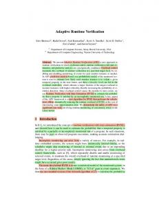
LBS vs. AP First we compare LBS to APdef ault , the configuration used in [27](K=V=4), and APxmt (K=1, V=4), the optimal configuration for XMT. We found the values of K and V for APxmt

s

SWS SI

80

FW

SP1

100

t ul

SPex/ex

SPtr/ex LBS

120

m

APdef ault APxmt SPtr/ex

Figure 6: Comparing LBS to SPtr/ex

nv co

LBS1

Description LBS (with ppt automatically determined by compiler) // Recommended Method LBS with ppt=1 // Not Recommended; For comparison only. AP with K=V=4 as in [27] AP with K=1, V=4, the best configuration for XMT SP with sst manually determined on training dataset and run on the execution dataset // Realistic SP with sst manually determined on execution dataset; then run on execution dataset. // Unrealistic SP with the default TBB threshold sst = 1 // Not Recommended; For comparison only. Serializing Work-Stealing Serializing Inner parallelism

LBS vs. SPtr/ex We compare LBS and SP in their recommended configurations. For LBS this is when ppt is determined by the compiler. For SP this is when sst is manually tuned by the programmer using a training data set, and thereafter run on the execution dataset (SPtr/ex). Figure 6 shows that LBS is 19.5% better on average and only falls behind on tsp (by 2.2%). For the other benchmarks LBS is up to 65.7% better. This shows that LBS is not only easier to use since it needs no tuning, it also allows for more performanceportable code to any dataset (in this case ex) it sees for the first time, because, as we will see in our next comparison, the performance gap between LBS and SP diminishes when SP is tuned on the execution dataset.

at m

Name LBS

bf

Table 3: Summary of Compared Configurations

FW

We compared our LBS scheduler against several other configurations shown in Table 3. All the compared approaches use the efficient hardware scheduler for outer parallelism provided by XMT.

0

nv

5.1 Results

50

co

Table 2 describes the training and execution datasets used for our experiments, as well as the manually determined sst for each dataset for SP, and the compiler determined ppt for LBS. For SP the smaller dataset is chosen as the training set, since typically programmers will use a smaller dataset for training given its time consuming and tedious nature. LBS and AP need no training.

100

t

1 1

150

ul

91 108 53 77

200

m

tsp queens

LBS ppt 1 1

APxmt APdefault LBS

250

at

FW qs bfs SpMV

Execution Set Size sst 512x512 1 1K 2 image, 1 162 filter 512 nodes 64 1M 256 G(10K,8M) 64 80Kx5K, 64 40M non-zero 11 nodes 1 N=11 1

300

m

Training Set (SP) Size sst 64x64 4 642 image, 1 162 filter 64 nodes 32 10K 16 G(10K,200K) 16 30Kx100, 4 60K non-zero 9 nodes 1 N=9 4

Name matmult conv

Figure 5: Comparing LBS to APxmt and APdef ault Run-time normalized vs. APxmt (%)

Table 2: Datasets and Thresholds.

by trying all nine configurations with K, V ∈ {1, 2, 4} and picking the one that gave the best average performance on our benchmarks. We noticed that varying V for a given choice of K affected performance negligibly, so we picked V=4. While K=1 is low, on XMT it is acceptable because it will only be applied to nested do-alls, since the outer do-all iterations are scheduled individually by the hardware. Figure 5 shows that LBS is 16.2% better than APxmt tuned for XMT, and 38.9% better than the default APdef ault with AP falling behind on the benchmarks with very fine-grain parallelism (FW, bfs and SpMV). For those benchmarks, a manually determined sst would be required to further reduce splitting in AP.

Run-time normalized vs. SPtr/ex (%)

solutions to placing N queens on an N × N chess-board so that no two queens can attack each-other. All benchmarks are coded in the most natural way, which is in line with our goal to provide good performance for natural programming idioms. tsp, queens and quicksort have recursively nested parallelism which is amenable to parallelism cut-off [13] (i.e., deciding to call a serial version of the recursive function from recursive depths greater than a threshold T ). For tsp and queens we set the cut-off threshold to T=N/2. For qs instead of using the depth of the recursion we use the size of the sub-array to be sorted or partitioned for the cut-off threshold: we call a serial quicksort when the subarray has less than 100 elements, and serial partition when the subarray has less than T = 3 #PNrocs elements. This last threshold is more complicated because the parallel partition code performs almost three times more work than the serial version; so we want to call the parallel version only when several processors are likely to be idle, such as at the onset of execution. Even with such a high partition cut-off threshold, always calling the serial partition is faster for SWS, SI, and SP with sst=1. In those cases we always call the serial partition.

LBS vs. SPex/ex Next, Figure 7 compares LBS to the hypothetical best case for SP: when SP is both tuned and run on the same execution dataset (SPex/ex ). This SPex/ex case is not realistic since it makes no sense for the user of the program to tune SP for each new dataset that comes by, since typically datasets are different in each run in deployment. After all, multiple tuning runs are a waste, since after the first run of a dataset the program produces the required answer, and no further runs are needed. This result is nevertheless presented to show that even in the ideal case for SP with idealized manual tuning on every new dataset, LBS (without tuning) still runs faster than SPex/ex by 3.8%, and falls behind only on tsp (by 2.2%). This means that even in rare cases that the datasets for an application have nearly identical characteristics, LBS is still a better choice – it is slightly faster,

SPex/ex LBS

120 100 80 60 40 20 0

(g G eo

t

ns

ul

V

ee

AV

qs

qu

M

p ts

Sp

s bf

FW

nv

m at

co

m

Run-time normalized vs. SPex/ex (%)

Figure 7: Comparing LBS to SPex/ex

m )

40 20 0

)

m

eo

(g

G

ns

ee

AV

qs

qu

V

M

p

ts

Sp

s

bf

FW

t

Run-time normalized vs. SP1 (%)

60

ul

80

80

nv

100

100

m

120

SI LBS+

120

co

SP1 SWS LBS1 LBS

140

140

at

Figure 8: Comparing LBS and LBS1 to SP1 and SWS

Figure 9: Comparing LBS+ to SI

m

LBS and LBS1 vs. SP1 and SWS Figure 8 first compares LBS, SP, and SWS in their best configurations that do not require any tuning, which are LBS, SP1 and SWS, respectively. The goal is to compare performance at a constant user effort-level. SP is the only one of the three that needs tuning, and its best suggested configuration without tuning is SP1 , when the sst threshold is set to 1 (this is the default value in Intel’s TBB when the user chooses not to do any tuning). SWS is the serialized work stealing scheme. Among these three (LBS, SP1 , and SWS), it is no surprise that LBS vastly outperforms the other two, by 56.7% and 54.7%, respectively, showing that without tuning, LBS is the best choice. We also present results for LBS1 in Figure 8 to present an interesting (but not necessarily very meaningful) comparison between LBS1 and SP1 . Neither has any compile-time restriction on splitting, and the comparison isolates the gain from the run-time adaptivity in LBS alone, which the figure shows is an impressive 47.2%. However since both LBS and SP are run in sub-optimal configurations, we should not read too much into this result. What is also interesting is that SP1 is never better than SWS which confirms our analysis in Table 1: when sst = 1 SP performs approximately 3/2 more transactions than SWS in the intermediate and best cases. It is important to recognize however that XMT’s hardware scheduling of outer do-all loops practically eliminates the serialization of TD accesses problem of SWS. Had we used a different platform SWS might have been worse than SP1 .

running the software scheduler (LBS) was excessive. But because the bounds of the do-all loop were known at compile time, the compiler decided that it is not profitable to parallelize it and chose to serialize it. LBS+ includes this additional optimization. For bfs and SpMV the situation is more complex because the bounds of the inner do-all loops are only known at run-time just before they are executed. Our compiler injects a check in the code just before the inner do-all loop to decide whether to run a serialized clone of the inner do-all or the original parallel one. This decision is based on the number of iterations of the do-all loop and on an statically determined estimate of the amount of computation (in cycles) each iteration will perform. We run the parallel version when the total estimated computation of the do-all exceeds ten thousand cycles. We call this configuration LBS+ to distinguish it from the LBS configuration we used so far where the optimization of static and dynamic serialization of inner parallelism was turned off to make the comparison to the other approaches fairer. Note that LBS+ and LBS are different only for FW, bfs and SpMV. Figure 9 shows that LBS+ outperforms SI by 54.2% on average, doing much better than SI on code without enough outer parallelism (tsp, queens, qs) and doing as well as SI on code with longer iterations (matmult, conv). LBS+ still falls behind on bfs and SpMV because the injected check to decide whether to run the parallel or serialized version of the do-all loop can take several tens of cycles (because it needs to access memory locations) which might be a significant enough percentage of the computation of the inner doall. Overall however, injecting the checks is beneficial.

Run-time normalized vs. SI (%)

and a lot easier to use since no tuning is required. The greater gap between LBS and SPtr/ex compared to SPex/ex shows the greater portability of LBS to new datasets and run-time conditions.

Scalability and Speedups Table 4 shows speedups of LBS+ run all 64 TCUs (parallel cores) compared to running the same parallel program with LBS+ on one TCU of the XMT prototype. The average speedup of 62.3x shows that LBS+ scales well to a significant number of cores. Some of the speedups are super-linear which is explained by complex cache behavior causing more cache misses when only one TCU is active. Table 4: Speedups of LBS+ vs. Parallel Program on 1 TCU

60

matmult 70.5

40 20

conv 67.2

FW 54.7

bfs 63.2

SpMV 60.7

tsp 67.5

queens 62.5

qs 52.1

Average Speedup (arithmetic): 62.3

0

G AV

qs s

t

) om

e (g

V

n ee

qu

p

ts

M Sp

s

bf

FW

nv

ul m at

co

m

LBS+ vs. SI Serializing Inner parallelism (SI) simply serializes all inner do-all loops. Since it is an easy way to provide some support for nested parallelism, it has been adopted by some OpenMP implementations. We found that although LBS outperforms SI substantially on average, for three benchmarks (FW, bfs and SpMV) LBS falls behind. The worst was FW where LBS was performing much worse than SI because the inner parallelism was extremely fine-grained and regular and the overhead of even creating TDs and

We also present speedups of our programs compared to an optimized serial version that runs on the powerful MTCU of XMT in Table 5. While the previous numbers reveal how well LBS scales to many cores, these numbers show the attainable performance. It is fairer to judge performance using these numbers for two reasons: TCUs are much simpler, more light-weight processors compared to the MTCU which is a powerful serial core that should be our baseline, but also a serial program is usually simpler and requires less computation than its parallel counterpart. For example in tsp the parallel version uses dynamic memory allocation to build possible solutions in parallel, whereas the serial version can use

a single, statically declared array, which is why tsp has a smaller speedup than other benchmarks. Table 5: Speedups of LBS+ vs. Serial Program on MTCU matmult 63.9

conv 28.2

FW 37.6

bfs 12.8

SpMV 26.0

tsp 11.1

queens 20.1

qs 6.9

Average Speedup (arithmetic): 25.8 Overall, the average speedup of 25.8x is impressive given that the serial code is more efficient, the MTCU is much more powerful than the TCUs, and that several of our benchmarks are irregular and hard to parallelize. Unlike on XMT, for many other platforms and compilers, irregular benchmarks yield little or no speedup with parallelism.

6. Related Work In this section we present previous work on two types of schedulers: i.) schedulers that support parallel function calls or futures but not do-all loops, ii.) schedulers that explicitly support do-all loops. Then we present work on throttling parallelism: serializing parallelism at run-time to minimize overheads. Non Do-All Loop Schedulers. These approaches don’t explicitly support do-all loops; instead they introduce parallelism through function calls or futures. Handling of do-all loops explicitly opens optimization opportunities not available to parallel function calls, since do-all loops create many iterations simultaneously, instead of one at a time. Multiple iterations can be packaged into a single TD, greatly reducing the number of TD transactions, and leading to much better performance. Work stealers that don’t explicitly support do-all loops do not optimize for them and deliver much inferior performance. This explains why EBS is our primary competitor since it explicitly supports do-all loops. Nevertheless, methods for parallel function calls are outlined below. Cilk[15] implements work-stealing but was designed for parallel function calls (i.e. relatively coarse-grain parallelism) and is not optimized for do-all loops. We have adopted a Cilk-like implementation which we call serialized work stealing (SWS), which our results show performs much worse than LBS for do-all loops. This result is not surprising since Cilk was not meant for do-alls. Other approaches that focus on coarser parallelism, such as parallel function calls and futures, [19, 24, 16, 29] have the same limitations. Arora et al.[4] propose a non-blocking implementation of workstealing which is well suited for multiprogrammed systems. Their approach suffers from deque overflows which can cause the program to crash. Two other approaches [17, 12] propose complicated solutions to the overflow problem. LBS overcomes this problem simply by implementing deques as constant-size circular arrays and keeping work (TDs) temporarily on the stack if the deque is full. Hendler et al. [18] propose stealing half the TDs of a deque instead of just one, so as to better spread the work across the system, and prove good theoretical bounds for load-balance. Their approach is not applicable to LBS because each deque will have at most one TD at all times. Goldstein et al.[16] propose a lightweight thread creation mechanism for nested parallelism which has the same serializing problem as SWS because it relies on the parent thread activating nascent threads upon request by a remote processor, to make them available for execution on the remote processor. Do-All Loop Schedulers Among the related work schemes, the only ones that we are aware of that explicitly support do-all loops by work-stealing are SP and AP in Intel’s TBB [1] and Cilk++[21] which apparently implements SP1 . As explained, to use SP the programmer is expected to determine a good value for the stopsplitting-threshold of each do-all loop, by trying out various val-

ues. Moreover this fixed threshold limits the performance portability of the code to a different number of cores, datasets and contexts. LBS frees the programmer from choosing a threshold manually and adapts to run-time conditions to avoid excessive splitting, without falling behind on performance. AP does not require programmer tuning but it still falls behind LBS because it lacks context portability, as it is not run-time adaptive. Finally SP1 falls significantly behind on code with fine-grain parallelism. The rest of the schedulers in this sub-section support do-all loops, but are not work stealing methods. OpenMP [26] recognizes the need for nested parallelism by providing primitives, but whether nesting is truly supported or not is implementation specific. Frequently OpenMP implementations serialize inner parallelism which our results show has serious performance limitations. The nano-threads library supports nested parallelism [22] and can be used for OpenMP, but uses a ready queue, or a hierarchical ready queue [25] for scheduling, both of which can have an arbitrarily higher memory footprint than work-stealing. Additionally, access to the head or tail of a queue must be synchronized among all threads, and a hierarchical ready queue (a tree of queues) has a single enqueue point, the root, and requires multiple operations to get work to the leaves where it is dequeued. This makes them unsuitable for our goal of scalable fine-grain parallelism. Duran et al.[14] propose a system that assigns processors to tasks by instrumenting the code and getting run-time statistics to refine the distribution. They assume however that the programmer has clustered the outer parallelism into ngroups (similar to setting the sst), and has also defined the grain-size (sst) of the inner parallelism. Our scheme does not need to collect run-time statistics, and does not place the burden of clustering on the programmer. NESL[7] employs complex compiler transformations to support nested parallelism by flattening[8]. NESL is an interpreted functional language without side-effects which limits its scope. Moreover, it is unclear if good performance can be achieved since only three benchmarks are evaluated (only one with nested parallelism) on three architectures, and in most cases their approach falls behind native code for these machines. The claim is that much better performance will be achieved if the language is compiled instead of interpreted, but we are unaware of a study quantifying this claim. Parallelism Throttling Some have used run-time conditions to decide whether to create more parallelism or execute work serially [19, 11]. Unlike them we do not rely on maintaining extra information (e.g., a global counter) indicating the state of the system and accessing it to make serializing decisions, which creates a hot-spot and doesn’t scale well. Instead LBS only uses local per-core information already available avoiding extra overheads and creating a hot-spot. Moreover, unlike both approaches that make irrevocable serialization decisions, LBS only postpones parallelism creation by running a few iterations before rechecking the system load. Duran et al.[13] propose an interesting way to limit the creation of excessive parallelism which is not related to scheduling. In fact they experiment with several schedulers to show that their method works well with all of them. They inject code that collects statistics about the amount of work of different procedures as a function of the depth (of the call-stack) at which they are called. When enough statistics are collected, they turn off this profiling and use the information to decide which procedures to serialize and at what depth. Given a recursive parallel procedure such as quicksort, their approach will decide at which depth of the recursion to start calling a serial version of quicksort. This approach is orthogonal to LBS because it does not solve the need to schedule the work, and can be applied on top of it. In fact our recursively nested benchmarks (tsp, queens, qs) have manual parallelism cut-off which achieves the same performance benefits as Duran’s scheme. As our results show, even for these benchmarks, LBS was able to schedule the

remaining parallelism more efficiently than some of the competing schedulers without falling behind (on average) compared to the others. It is important to note, however, that parallelism cut-off is not applicable to all programs.

7. Conclusion We have presented Lazy Binary Splitting, a work-stealing scheduler that builds on Eager Binary Splitting and compared it to the two EBS alternatives offered by TBB, SP and AP. LBS performs better in the typical SPtr/ex case and doesn’t fall behind in the idealized but unrealistic SPex/ex case. Unlike SP, LBS does not require manual tuning and is performance portable. AP improves on SP by not requiring manual tuning and being performance portable across datasets and platforms, but it lacks context portability. That is why LBS, which is context portable, outperforms AP.

References [1] Intel Threading Building Blocks Reference Manual, Rev. 1.9, 2008. [2] Umut A. Acar, Guy E. Blelloch, and Robert D. Blumofe. The data locality of work stealing. In SPAA ’00: Proceedings of the 12th annual ACM symposium on Parallel algorithms and architectures, 2000. [3] Kunal Agrawal, Yuxiong He, and Charles E. Leiserson. Adaptive work stealing with parallelism feedback. In PPoPP ’07: Proceedings of the 12th ACM SIGPLAN symposium on Principles and practice of parallel programming, 2007. [4] Nimar S. Arora, Robert D. Blumofe, and C. Greg Plaxton. Thread scheduling for multiprogrammed multiprocessors. In Proc. of the 10th annual ACM symp. on Parallel algorithms and architectures, 1998. [5] Krste Asanovic, Ras Bodik, Bryan Christopher Catanzaro, Joseph James Gebis, Parry Husbands, Kurt Keutzer, David A. Patterson, William Lester Plishker, John Shalf, Samuel Webb Williams, and Katherine A. Yelick. The landscape of parallel computing research: A view from berkeley. Technical Report UCB/EECS-2006-183, EECS Department, Berkeley, Dec 2006. [6] Aydin O. Balkan, Gang Qu, and Uzi Vishkin. A mesh-of-trees interconnection network for single-chip parallel processing. In ASAP ’06: Proceedings of the IEEE 17th International Conference on Application-specific Systems, Architectures and Processors, 2006. [7] Guy E. Blelloch, Jonathan C. Hardwick, Siddhartha Chatterjee, Jay Sipelstein, and Marco Zagha. Implementation of a portable nested data-parallel language. In Proceedings of the fourth ACM SIGPLAN symposium on Principles and practice of parallel programming, 1993. [8] Guy E. Blelloch and Gary W. Sabot. Compiling collection-oriented languages onto massively parallel computers. J. Parallel Distrib. Comput., 8(2):119–134, 1990. [9] Robert D. Blumofe and Charles E. Leiserson. Scheduling multithreaded computations by work stealing. J. ACM, 46(5), 1999. [10] George C. Caragea, A. Beliz Saybasili, Xingzhi Wen, and Uzi Vishkin. Brief announcement: performance potential of an easy-to-program PRAM-on-chip prototype versus state-of-the-art processor. In SPAA ’09: Proceedings of the twenty-first annual symposium on Parallelism in algorithms and architectures, 2009. [11] Olivier Certner, Zheng Li, Pierre Palatin, Olivier Temam, Frederic Arzel, and Nathalie Drach. A practical approach for reconciling high and predictable performance in non-regular parallel programs. In DATE ’08: Proceedings of the conference on Design, automation and test in Europe, 2008. [12] David Chase and Yossi Lev. Dynamic circular work-stealing deque. In SPAA ’05: Proceedings of the 17th annual ACM symposium on Parallelism in algorithms and architectures, 2005. [13] Alejandro Duran, Julita Corbal´an, and Eduard Ayguad´e. An adaptive cut-off for task parallelism. In SC ’08: Proceedings of the 2008 ACM/IEEE conference on Supercomputing, 2008.

[14] Alejandro Duran, Marc Gonz`alez, and Julita Corbal´an. Automatic thread distribution for nested parallelism in OpenMP. In ICS ’05: Proc. of the 19th annual international conf. on Supercomputing, 2005. [15] Matteo Frigo, Charles E. Leiserson, and Keith H. Randall. The implementation of the Cilk-5 multithreaded language. In PLDI ’98: Proceedings of the ACM SIGPLAN 1998 conference on Programming language design and implementation, 1998. [16] Seth Copen Goldstein, Klaus Erik Schauser, and David E. Culler. Lazy threads: implementing a fast parallel call. Journal of Parallel and Distributed Computing, 37(1):5–20, 1996. [17] Danny Hendler, Yossi Lev, and Nir Shavit. Dynamic memory ABP work-stealing. In DISC, pages 188–200, 2004. [18] Danny Hendler and Nir Shavit. Non-blocking steal-half work queues. In PODC ’02: Proceedings of the twenty-first annual symposium on Principles of distributed computing, 2002. [19] D. A. Kranz, Jr. R. H. Halstead, and E. Mohr. Mul-t: a highperformance parallel lisp. SIGPLAN Not., 24(7):81–90, 1989. [20] Alexey Kukanov and Michael Voss. The foundations for scalable multi-core software in intel threading building blocks. Intel Technology Journal, 11(04), November 2007. [21] C.E. Leiserson. The Cilk++ concurrency platform. In Design Automation Conference, 2009. DAC ’09. 46th ACM/IEEE, July 2009. [22] Xavier Martorell, Eduard Ayguad´e, Nacho Navarro, Julita Corbal´an, Marc Gonz´alez, and Jes´us Labarta. Thread fork/join techniques for multi-level parallelism exploitation in NUMA multiprocessors. In ICS ’99: Proc. of the 13th international conf. on Supercomputing, 1999. [23] Maged M. Michael, Martin T. Vechev, and Vijay A. Saraswat. Idempotent work stealing. In PPoPP’09: Proc. of the 14th ACM SIGPLAN symp. on Principles and practice of parallel programming, 2009. [24] Eric Mohr, David A. Kranz, and Jr. Robert H. Halstead. Lazy task creation: a technique for increasing the granularity of parallel programs. In LFP ’90: Proceedings of the 1990 ACM conference on LISP and functional programming, 1990. [25] Dimitrios S. Nikolopoulos, Eleftherios D. Polychronopoulos, and Theodore S. Papatheodorou. Efficient runtime thread management for the nano-threads programming model. In Proceedings of the 2nd IEEE IPPS/SPDP Workshop on Runtime Systems for Parallel Programming, LNCS, pages 183–194, 1998. [26] OpenMP Architecture Review Board. OpenMP Application Program Interface, Ver. 3.0 May 2008. http://www.openmp.org. [27] A. Robison, M. Voss, and A. Kukanov. Optimization via reflection on work stealing in TBB. In IPDPS 2008: IEEE International Symposium on Parallel and Distributed Processing, 2008. [28] A. Beliz Saybasili, Alexandros Tzannes, Bernard R. Brooks, and Uzi Vishkin. Highly parallel multi-dimentional fast fourier transform on fine- and coarse-grained many-core approaches. In PDCS ’09: The 21st IASTED International Conference on Parallel and Distributed Computing and Systems, 2009. [29] Kenjiro Taura, Kunio Tabata, and Akinori Yonezawa. StackThreads/MP: integrating futures into calling standards. In PPoPP ’99: Proceedings of the seventh ACM SIGPLAN symposium on Principles and practice of parallel programming, 1999. [30] Shane Torbert, Ron Tzur Uzi Vishkin, and David Ellison. Is teaching parallel algorithmic thinking to high-school student possible? one teachers experience. In Proc. 41st ACM Technical Symposium on Computer Science Education (SIG CSE) (To Appear), 2010. [31] Uzi Vishkin, George C. Caragea, and Bryant C. Lee. Handbook of Parallel Computing: Models, Algorithms and Applications, chapter Models for Advancing PRAM and Other Algorithms into Parallel Programs for a PRAM-On-Chip Platform. CRC Press. Rajasekaran, R., and Reif, J. Eds, 2008. [32] Xingzhi Wen and Uzi Vishkin. FPGA-based prototype of a PRAMon-chip processor. In CF ’08: Proceedings of the 5th international conference on Computing frontiers, 2008.