Lazy Propagation in Junction Trees
Anders L. Madsen
Finn V. Jensen
Department of Computer Science Aalborg University Denmark
[email protected]
Department of Computer Science Aalborg University Denmark
[email protected]
Abstract The efficiency of algorithms using secondary structures for probabilistic inference in Bayesian networks can be improved by exploiting independence relations induced by evidence and the direction of the links in the original network. In this paper we present an algorithm that on-line exploits independence relations induced by evidence and the direction of the links in the original network to reduce both time and space costs. Instead of multiplying the conditional probability distributions for the various cliques, we determine on-line which potentials to multiply when a message is to be produced. The performance improvement of the algorithm is emphasized through empirical evaluations involving large real world Bayesian networks, and we compare the method with the HUGIN and Shafer-Shenoy inference algorithms.
1
specific information scenaria, a careful exploitation of the d-separation properties would result in less complex structures. Consider for example the Bayesian network indicated in figure 1. If A is instantiated and no evidence has been entered to DAG4, then DAG1, DAG2, and DAGj are independent, and we need only sent messages down to DAG4. An on-line triangulation of this scenario will result in a much simpler set of junction trees than the off-line produced junction tree. To exploit the specific independences, we need a very efficient algorithm for detecting independences and to perform an efficient triangulation based on these independence~. In particular, as the problem of optimal triangulation is NP-complete, there is not much hope that a method requiring on-line triangulation can outperform the "standard" methods for large networks, and improved performance for small networks is not particularly interesting.
Introduction
It has for a long time been a puzzle why "standard" inference algorithms for Bayesian networks did not really use the direction of the links in the network. By "standard" we mean the LauritzenSpiegelhalter [Lauritzen and Spiegelhalter, 19881, the Shafer-Shenoy [Shafer and Shenoy, 19901, and the HUGIN[Jensen et al., 19901 algorithms and the various variations over these algorithms ( [Shachter, 19901 and [Jensen, 19951). These algorithms build a secondary structure (a junction tree or a join tree) by triangulating the (moralized) network. This structure can be used for propagation for all information scenaria. Therefore, the algorithms do not exploit independences induced by the evidence. That is, the tree-structure is large enough to take care of all instantiations of variables. For some (or sometimes all)
Figure 1: If A is instantiated and no evidence has been entered to DAG4, then it is only necessary to sent messages down to DAG4. We may relax the requirement to the updating algorithm such that we are only interested in updated probabilities for a very small set of variables. In that case the SPI method [Shachter et al., 19901 and the bucket sort algorithm [Dechter, 19961 can utilize specific independences, as they consist of a collect operation only, where the variables are successively eliminated by multiplying the functions involving A (say)
Lazy Propagation in JunctionTrees
and marginalizing A out of this product. These methods, however, are not able to update all variables efficiently. In this paper we propose a compromise between off-line triangulation and on-line exploitation of specific independences. We call the method lazy propagation as the bulk of the method is lazy evaluation of the potentials for cliques and separators. That is, we work with an off-line produced junction tree, where we have allowed ourselves to use much time on finding a small junction tree. Now, instead of multiplying the conditional probability distributions for the various cliques, we determine on-line which potentials to multiply when a message is to be produced. Thereby, when a message is to be produced, only the required functions are multiplied. An effect of this scheme is that d-separation properties induced by evidence are automatically exploited. The rest of the paper is organized in the following way. Section 2 describes the lazy propagation scheme in detail. In section 3 we present results from a series of real-time tests performed. A discussion of the results is given in section 4, and in section 5 we illustrate how d-separation properties are automatically exploited.
2
Methods
We briefly review the HUGINand the Shafer-Shenoy algorithms. For more elaborate presentations, see the references above. A Bayesian network consists of a graph G = (V, E) and a probability distribution P. G is a directed acyclic graph, V is the set of variables (which are assumed to be discrete), and E is the set of edges connecting the variables. The probability distribution P factorizes on G such that:
P=
1 -P ( V lpa(V)), VEV
where pa(V) is the parent set of V. The secondary structures used by the HUGINand Shafer-Shenoy architectures are constructed from G. A junction tree representation of a Bayesian network G is constructed by moralization and triangulation of G. The nodes of the junction tree correspond to cliques of the triangulated graph. A clique is a maximal connected subgraph of the triangulated graph. The cliques of the junction tree are connected by separators such that the so-called junction tree property holds. The junction tree property insures that whenever two cliques Ciand Cjare connected by a path, the intersection, Cin Cj is a subset of every clique and separator on the path. To each clique C and each
363
separator S we associate potentials dc and ds, respectively. dc and ds are functions having the variables of C and S as domains. Each variable, V, in the Bayesian network has a conditional probability distribution P ( V I pa(V)). Every distribution is assigned to a clique such that the domain of the distribution is a subset of the clique domain. The set of distributions assigned to a clique, C, are combined to form the potential function 'Jlc. Initially the potentials of the junction tree are given as:
dc =lltc
and
4s = 1
for each clique, C, and each separator, S.
Figure 2: Cliques Ciand Cjare connected by the s e p arator S = Ci n Cj. The propagation of evidence in the HUGINarchitecture is based on the operation of absorption. Assume Ci and Cj to be neighboring cliques in a junction tree with S as separator, see figure 2. We say that Cj absorbs from Ci if we: calculate
4: =
dc,; Ci\S
give S the potential
4:;
give Cjthe potential
4: dzj = dcj -. 4s
The absorption operation is used when a message is sent from one clique to another. Messages flow in two recursive phases, and the flow is controlled by choosing a root clique of the junction tree. The first phase is initiated by collecting evidence to the root and the second phase is initiated by distributing evidence from the root. Collection of evidence to a clique C is done by collecting - evidence to all the children of C followed by absorption of evidence from each child. Similarly, distribution of evidence from a clique amounts to absorption of evidence into each child followed by distribution of evidence from the child. After a full round of message passing a message has been sent in each direction along every separator in the junction tree. The Shafer-Shenoy algorithm can perform inference in a junction tree. The reader should notice that the Shafer-Shenoy algorithm propagates evidence faster in binary join trees than in junction trees [Shenoy, 19971. The Shafer-Shenoy inference architecture differs from
364
Madsen and Jensen
the HUGINarchitecture in a number of ways. First, the flow of messages is not controlled by choosing a root of the junction tree. A clique sends asynchronously a message to one of its neighbors when messages from all other neighbors have been received. Second, the clique potentials are not updated during propagation of evidence instead each separator holds two messages. One for each direction. Third, no division of potentials is performed. Consider figure 2 once again. The Shafer-Shenoy message, c$ci+cj,sent from Cito Cjis calculated as:
where $ci is the clique potential of set of neighbors to Ci.
Ci and Nci is the
After a full round of message passing in the ShaferShenoy architecture each separator holds two messages. The clique potential dci can be obtained by taking the product of all messages sent to Ci and $ci. The message passing scheme for asynchronous firing corresponds to the scheme of CollectEvidence followed by DistributeEvidence. The root is, however, chosen randomly. Let the separator, S, between cliques Ci and Cjbe the first separator over which messages are sent in both directions, see figure 3. Before Cj sent the message, new, over S, it has received a message from all its neighbors. This is equivalent to collecting evidence to Cj.Sending messages from Cjto all its neighbors is equivalent to distributing evidence from
the number of arcs in the graph. The posterior distribution of the target set is equal to the product of the distributions of the relevant nodes marginalized down to the target set.
2.1
Lazy Propagation
The basic idea behind lazy propagation is to take advantage of two important properties of the potentials associated with the nodes of the Bayesian network:
the d-separation criterion applies to the potentials. Instead of combining the probability distributions associated with a clique to obtain the clique potential, we keep the clique potential in factored form, and we change the content of messages passed between cliques in the junction tree. Instead of sending a message consisting of one potential with the set of separator variables as domain, we sent a message consisting of a set of potentials all having domains which are subsets of the separator domain. Messages can flow as in the asynchronous firing scheme or may be controlled by choosing a root as in the HUGINarchitecture.
cj. new
Figure 3: If Cjis the first clique to receive a message from all its neighbors in asynchronous firing, then the messages sent are the same as the messages sent when collecting evidence to Cj. The SPI algorithm and the bucket elimination algorithm do not perform inference based on a secondary structure. Both algorithms are most advantageously used if the reasoning is focused in the sense that only the posterior probability distributions of a small set of target variables are to be calculated. The basic idea behind the SPI and the bucket elimination algorithms is to consider only variables relevant to reasoning about the target set. The variables relevant for a query can be determined from the original Bayesian network by an algorithm which runs in time linear in
Figure 4: A Bayesian network. Lines without direction are fill ins added during triangulation of the network. Consider the Bayesian network shown in figure 4 and the corresponding junction tree shown in figure 5. Assume that variable A is instantiated by evidence. Each potential with A in its domain has the domain decreased by A. If we assume potentials to be represented as tables, then P* is the subtable of P corresponding to the instantiation of A. In figure 6 we follow the flow of messages from the leaves of the junction tree towards ABF in the lazy propagation scheme. The message flow corresponds to collecting evidence to ABF in the HUGINarchitecture. Assume that the first leaf to sent a message is EFH. The potential associated with this clique is P(H I E, F ) . Variable H has to be eliminated, but no calculations are required as C HP ( H I E , F ) = l E P .
Lazy Propagation in JunctionTrees
365
tentials sent from A D F to D F G are P ( F ) and P*(D). At D F G we have to combine P*(D) and P ( G I D) and marginalize D out to obtain the message to send to F G I . BEF is the last child of A B F to receive a message, and the message sent consists of P*(B) and P ( F ) . Finally, a message containing P ( F ) and P ( E ) = C , P ( E I B)P* (B) is sent to E F H .
(F),P(E)=:
Figure 5: A junction tree constructed from the Bayesian network shown in figure 4. Prior distributions are assigned to cliques as indicated. The same argument is used when messages are sent from BEF, F G I , DFG, and ADF. The last clique to send a message is ACF. A C F has P*(C) and P ( F I C ) associated, and variable C is eliminated by taking the product of the two potentials and then marginalizing down to F.
~ ( EB)P'(B) I P(GID)
Figure 7: Shows the message flow in the junction tree during the second phase of lazy propagation. The initial messages are sent from ABF. It is not necessary to send the potentials containing only ones. We have included these potentials in the description to make the explanation clear. So, for this example we only performed three marginalizations and all of them involved only two variables.
Figure 8: The message sent from Ci to Cj consists of potentials f o i l . .. , fD, and the message sent in the opposite direction consists of
fDj - .. f ~ , . 1
Figure 6: Shows the message flow in the junction tree during the first phase of lazy propagation. The initial messages are sent from the leaves. At the end of the inward pass, potentials P*(B) and P ( F ) are associated with ABF. In figure 7 we follow the message flow in the opposite direction. The message sent from A B F to A C F is an empty message as none of the potentials associated with A B F needs to be sent to ACF. P ( F ) is the only potential relevant, but it was sent in the opposite direction during the inward pass of the algorithm (in HUGINterms it is divided out, in Shafer-Shenoy terms it shall not be transmitted). The message sent from A B F to A D F consists of the potential P ( F ) as no other potentials are relevant for the subtree rooted at ADF. The po-
1
The HUGINarchitecture imposes a division of separator potentials as described above. The lazy propagation scheme does not require this division, because the combination of potentials is postponed. Consider the two neighboring cliques shown in figure 8, and assume that the message sent from Ci to Cj over the separator S consists of the potentials f o i l . . . ,fD, and assume the message sent in the opposite direction to consist of the potentials f o j , . . . ,fDm. None of the poten, involved in any marginalization tials foil.. . ,f ~ are when sending from Cj to Ci. That is, foil... ,fD, C foj,.. . ,f ~ ,,and the division operation required in HUGINpropagation quite simply amounts to discard, foj,... ,f~,,, . So, lazy propaing f ~ ;. .,. ,f ~ from gation dissolves the difference between HUGINpropagation and Shafer-Shenoy propagation.
366
3
Madsen and Jensen
Empirical Results
We have tested the lazy propagation scheme to investigate how performance varies with the number of instantiated variables. To get an idea of the performance compared to standard schemes we have implemented Shafer-Shenoy as well as HUGINpropagation. The schemes implemented do only perform propagation. That is, the final step after propagation to marginalize the clique potentials down to each variable is not performed. Also, we have not implemented various speedup features, like binary join trees or 0-compression.
For a given Bayesian network we performed 50 propagations of evidence with the size of the evidence set fixed, but where the evidence variables were chosen at random before each propagation. The number of evidence variables varied from 0 to 50. Figure 9 describes four of the Bayesian networks and corresponding junction trees used for the tests. 10, 11, 12, and 13 show the average time cost of propagating evidence with the three schemes as a function of the number of variables instantiated in the Barley, the KK, the Diabetes, and the Mildew networks. The figures show that the average time cost of HUGINpropagation for this implementation is always smaller than the average time cost of Shafer-Shenoy propagation, and that the average time cost of lazy propagation decreases considerably as the number of instantiated variables increase.
Figure 10: A plot of the average time cost of propagating evidence in the Barley network as a function of the number of variables instantiated. The tests were performed on a Sun Ultra-2 workstation with two 300 MHz UltraSPARC-1 CPU's running Solaris 2.6 (SunOS 5.6). Each CPU has a 0.5 MB L2 cache. The total FtAM on the system is 1024 MB.
Figure 12: A plot of the average time cost of propagating evidence in the Diabetes network as a function of the number of variables instantiated. The average time cost of lazy propagation in the Barley, KK, and Mildew networks is smaller than the time cost of the other propagation algorithms even when no variables are instantiated. On average lazy prop agation in the Diabetes network becomes faster than Shafer-Shenoy propagation when 16 variables are instantiated, and faster than HUGINpropagation when 39 variables are instantiated.
4
Discussion
Figure 11: A plot of the average time cost of propagating evidence in the KK network as a function of the number of variables instantiated.
The experiments indicate that although some evidence may increase time costs, the overall effect of instantiating variables is a decrease of time costs, and with many variables instantiated, lazy propagation outperforms standard propagation schemes.
The algorithms were tested on different real-world Bayesian networks with different sizes of evidence sets.
It seems that time costs are in the same order of magnitude with no instantiated variables for all three
Lazy Propagation in JunctionTrees
Network KK Barley Diabetes Mildew
nodes 50 48 413 53
node potential size min p max 2 32256 2768.1 2 40320 2712.1 7056 1116.4 5 3 280000 15633.1
cliques 38 36 337 29
367
clique state space size clique neighbors p min p min max max 1 4 1.9 40 5806080 397780.2 1 4 1.9 216 7257600 481637.5 1 3 2.0 495 190080 30906.3 336 1756800 144133.0 1 3 1.9
Figure 9: Information on 4 Bayesian networks and the junction trees generated for these networks.
1. For each variable, V, not in the separator domain calculate the domain size of the potential obtained, if V is the next variable eliminated. A variable, V, is eliminated by combining all potentials including V in the domain and marginalizing v out. 2. Choose the next variable to eliminate as a variable resulting in the smallest domain size of the potential obtained.
Figure 13: A plot of the average time cost of propagating evidence in the Mildew network as a function of the number of variables instantiated.
schemes, and a rather small set of instantiated variables will yield lazy propagation faster than the standard schemes. f i r t h e r research is needed to quantify these statements We have only performed a limited number of tests to investigate how much the space costs are reduced. These tests indicate that the space costs are reduced considerably. This is expected as clique and separator potentials are represented in factored form. Time and space prevents us from giving a thorough elaboration of this topic. We have done little to speed-up the calculations of a message in the test implementation of lazy propagation. When a message has to be sent from one clique to another some variables have to be marginalized out. If we consider the domain graphs of the potentials relevant to the calculation of the message, then we are faced with a problem similar to the overall problem. That is, we have to calculate the joint probability of a set of nodes in the domain graph. Here any inference algorithm can be used. In the test implementation all relevant potentials are arranged in a list and variables not in the separator domain are eliminated one by one. Variables are eliminated according to the following peeling algorithm:
The algorithm is similar to the minimum clique weight heuristic for triangulation, but it is a little different. We do not always eliminate a variable V right away even though its neighbors form a complete graph as in the minimum clique weight heuristic. V is only eliminated right away if there is only one relevant potential containing V. The performance of the lazy propagation scheme depends very much on the topology of the junction tree. If the state spaces of the cliques and separators are large, the lazy evaluation architecture tends to be faster than the other two architectures for small sets of evidence. Sometimes the lazy evaluation architecture is faster even when no variables are instantiated. On the other hand, when the state spaces of the cliques and separators are small, large sets of evidence variables are required before the algorithm becomes faster. If a Bayesian network has many nodes without parents or many nodes without children, then speed-up is available even when no variables are instantiated. Let V be a variable without parents, then the marginal probability distribution of V can be sent over separators including V right away. Let W be a variable without children and assume that the potential of W is associated with clique C. When a message is sent from C over a separator not including W and W has not received evidence, then no calculations are necessary to eliminate W as:
This also applies in the more general case. That is, marginalizing out all head variables of a potential will
368
Madsen and Jensen
result in a unity potential with the tail variables as domain. Some sets of evidence decrease the performance of lazy propagation. Consider the Bayesian network shown in figure 14. A junction tree constructed from this network will contain cliques of the form DiEiFi for i = 1,... ,35, and these cliques are the only cliques containing Fi. No message has to be sent from a DiEiFi clique if variable Fi is not instantiated. If Fi is instantiated, then a message has to be sent from the DiEiFi clique. The lazy evaluation algorithm on average (n = 50) uses 4.2 seconds to propagate evidence when no variables are instantiated and 5.4 seconds when variables Fl,... ,F35are instantiated.
E are not d-separated. In figure 16 a junction tree for N is shown. For the internal elimination order in the cliques we use the peeling algorithm from section 4.
Figure 16: A junction tree for N. The potentials associated with the cliques are indicated. Now, assume that A is instantiated to a. In figure 17 we illustrate the flow of potentials towards the clique DE. The index of the potentials in the figure indicates the variables relevant for the calculation of the potentials. Index a indicates that the evidence A = a is relevant for the potential.
Figure 14: A Bayesian network used to illustrate how evidence might decrease the performance of lazy propagation. The concept of barren nodes was introduced in [Shachter, 19861 and are defined in [Liand Druzdzel, 19971 as nodes which are neither evidence nor target nodes and have no descendants or only barren descendants. According to this definition no nodes are barren in the lazy evaluation architecture as we are concerned with calculating the posterior probability distribution of all variables in the Bayesian network. The property of barren nodes exploited by algorithms such as the SPI algorithm is that barren nodes have no impact on the posterior probability distribution of the nodes in the target set. This property is exploited in the lazy propagation scheme as described in the next section.
5
d-separation and Lazy Propagation
Lazy propagation utilizes automatically d-separation properties induced by evidence. To illustrate this, consider the Bayesian network, N , in figure 15.
Figure 17: The flow of potentials to the clique D E when A is instantiated to a. As can be seen from figure 17, the evidence A = a is relevant for the updating of E. On the other hand, F is irrelevant for E, and this has caused a computational saving as the marginalization of F is costless. The cost of propagation is close to the cost of propagating in a junction tree for N\{F). Next, assume that also C is instantiated (to c). The flow of potentials is illustrated in figure 18. P(A), P(BI A)
P(CI B), P(DI C)
P ( E I D)
Figure 15: A Bayesian network, N, where A and E are independent given C. N has the properties that initially A and E are not d-separated. If C is instantiated, then A and E are dseparated, but if C and F are instantiated, then A and
Figure 18: The flow of potentials to the clique D E when A is instantiated to a and C to c. We see that only C = c is relevant for E, and the fact
Lazy Propagation in JunctionTrees
that E and A are d-separated has yielded substantial savings in the computation. No marginalizations are performed in the propagation. For completion we illustrate what happens when we furthermore instantiate F to f . Then A and E are not d-separated, and the resource requirements for updating DE increase.
369
tion: A unifying framework for probabilistic inference. In Horvitz, E. and Jensen, F., editors, Proceedings of the Twelfth Conference on Uncertainty in Artificial Intelligence, pages 211-219. [Jensen, 19951 Jensen, F. V. (1995). Cautious propagation in Bayesian networks. In Besnard, P. ant1 Hanks, S., editors, Proceedings of the Eleventh Conference on Uncertainty in Artificial Intelligence, pages 323-328. [Jensen et al., 19901 Jensen, F. V., Lauritzen, S. L., and Olesen, K. G. (1990). Bayesian updating in causal probabilistic networks by local computations. Computational Statistics Quarterly, 4:269-282.
Figure 19: The flow of potentials to the clique DE when A is instantiated to a, C to c, and F to f .
6
Conclusion
In this paper we presented an algorithm for probabilistic inference in Bayesian networks. The algorithm exploits the independences induced by evidence and the direction of the links in the original graph. The performance depends on the topology of the original Bayesian network and the junction tree constructed from it. The test results show that the algorithm performs inference faster than both the HUGINand the ShaferShenoy algorithms if the size of the set of evidence variables is large enough. It should, however, be emphasized that the performance of the test implementations of the Sllafer-Shenoy and the HUGINarchitedures can be improved by exploiting existing techniques for speeding up the algorithms. Most of these techniques also apply to the lazy evaluation architecture. The lazy propagation scheme enlarges the class of tractable Bayesian networks as the space costs of this scheme are smaller than the space costs of the HUGIN and Shafer-Shenoy architectures.
Acknowledgment Thanks to the anonymous referees for productive remarks and to the DINA-group at Aalborg University (http://www.cs.auc.dk/research/DSS/DINA).
References [Dechter, 19961 Dechter, R. (1996). Bucket elimina-
[Lauritzen and Spiegelhalter, 19881 Lauritzen, S. L. and Spiegelhalter, D. J. (1988). Local computations with probabilities on graphical structures and their application to expert systems. Journal of the Royal Statistical Society, B., 50(2):157-224. [Lin and Druzdzel, 19971 Lin, Y. and Druzdzel, M. J. (1997). Computational advantages of relevance reasoning in Bayesian belief networks. In Geiger, D. and Shenoy, P., editors, Proceedings of the Thirteenth Conference on Uncertainty in Artificial Intelligence, pages 342-350. [Shachter, 19861 Shachter, R. (1986). Evaluating influence diagrams. Operations Research, 34(6) 2371-882. [Shachter et al., 19901 Shachter, R., D'Ambrosio, B., and DelFavero, B. (1990). Symbolic probabilistic inference in belief networks. In Proceedings Eighth National Conference on AI, pages 126-131. [Shachter, 19901 Shachter, R. D. (1990). An ordered examination of influence diagrams. Networks, 20(5):535-563. [Shafer and Shenoy, 19901 Shafer, G. R. and Shenoy, P. P. (1990). Probability propagation. Annals of Mathematics and Artificial Intelligence, 2:327-352. [Shenoy, 19971 Shenoy, P. P. (1997). Binary join trees for computing marginals in the Shenoy-Shafer architecture. International Journal of Approximate Reasoning, 17(2-3) :239-263.