Learn Quantum Mechanics with Haskell - arXiv

Learn Quantum Mechanics with Haskell Scott N. Walck Department of Physics Lebanon Valley College Annville, Pennsylvania, USA [email protected]

To learn quantum mechanics, one must become adept in the use of various mathematical structures that make up the theory; one must also become familiar with some basic laboratory experiments that the theory is designed to explain. The laboratory ideas are naturally expressed in one language, and the theoretical ideas in another. We present a method for learning quantum mechanics that begins with a laboratory language for the description and simulation of simple but essential laboratory experiments, so that students can gain some intuition about the phenomena that a theory of quantum mechanics needs to explain. Then, in parallel with the introduction of the mathematical framework on which quantum mechanics is based, we introduce a calculational language for describing important mathematical objects and operations, allowing students to do calculations in quantum mechanics, including calculations that cannot be done by hand. Finally, we ask students to use the calculational language to implement a simplified version of the laboratory language, bringing together the theoretical and laboratory ideas.

1

Introduction

The theories of twentieth-century physics employ mathematical objects that are quite removed from our everyday experience of the world and surprisingly removed from the description of the experiments that led to or provided evidence for those theories. Certainly theoretical concepts have motivated and guided experiments—experimental design is awash in theory—but if we consider the simplest description of an experiment, as a chef might write a recipe for a lay cook, the language would not include references to the abstract objects that structure the theorist’s calculations. We focus in this paper on the theory of quantum mechanics, and in particular on the behavior of spin-1/2 particles, some of the very simplest quantum systems which nevertheless contain the essential features of quantum mechanics. We present a Haskell-based method for learning quantum mechanics that takes place within a senior-level quantum mechanics course. Students in the course may have no experience with Haskell or programming at all. We take the attitude of Papert[4] and others[8, 9, 1, 12] that students are aided in their learning by having building blocks with which to create interesting structures, that such creative activity is a motivating and effective way to learn, and that the feedback provided by computer-language-based building blocks can expose our confusions and produce delight in our achievements. The paper is organized as follows. In section 2, we introduce a laboratory language for the description of experiments with spin-1/2 particles. In section 3, we describe a calculational language for working with kets and operators, the abstract objects used to do calculations. In section 4, we describe a simplified laboratory language that students are asked to implement using the calculational language. J. Jeuring and J. McCarthy (Eds.): Trends in Functional Programming in Education (TFPIE) EPTCS 230, 2016, pp. 31–46, doi:10.4204/EPTCS.230.3

Learn Quantum Mechanics with Haskell

32

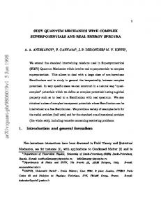
Inhomogeneous magnetic field Ag Oven

Figure 1: The Stern-Gerlach experiment.

2

Laboratory Language

The Stern-Gerlach experiment was performed by Otto Stern and Walther Gerlach in 1922, a time when the theory of quantum mechanics was being developed. The experiment demonstrates the quantization of angular momentum, which we now know comes in integer and half-integer multiples of h¯ , Planck’s constant. Several modern quantum mechanics textbooks begin the subject with the SternGerlach experiment.[7, 10, 6] The Feynman Lectures also introduce the Stern-Gerlach experiment early in the volume on quantum mechanics.[2] A schematic of the Stern-Gerlach experiment is shown in Figure 1. Silver (Ag) atoms are heated in an oven and made into a beam by passing through small holes. Stern and Gerlach chose silver because, with a single electron in its outer shell, it mimics the magnetic behavior of an electron. The electron and the silver atom each possess a magnetic dipole moment, that is, they behave like tiny bar magnets in the presence of a magnetic field. Such a magnetic dipole moment will feel a torque, an urge to rotate, in the presence of a magnetic field, and will moreover feel a force if the magnetic field is inhomogeneous, changing from one position in space to another. The Stern-Gerlach experiment aims to produce a force on the silver atoms with an inhomogeneous magnetic field oriented in a particular direction, say the z direction. The silver atoms in the beam are then expected to deflect upward or downward in the z direction, depending on the extent to which their magnetic dipole moments (vectors oriented along the imagined tiny bar magnets) point in the negative or positive z direction. Classical (pre-quantum) physics predicts that the random distribution of magnetic dipole moments coming from the oven should produce a continuous spectrum of deflection of the silver atom beam. Instead, what is seen in the experiment is that the beam splits into two beams, and produces two spots on a detecting screen. Gerlach called this “directional quantization”[10], and, since magnetic dipole moment is proportional to angular momentum, we now think of this as quantization of angular momentum. The electron and the silver atom are called spin-1/2 particles because the z-component of angular momentum for particles in one of the two beams is (1/2)¯h, and that in other beam is −(1/2)¯h. Spin-1/2 particles are particles that have two outcomes in a Stern-Gerlach experiment (as such, they are examples of quantum bits, or qubits). Although we won’t talk about them in this paper, it may be helpful to know that spin-1 particles have three outcomes in a Stern-Gerlach type experiment, spin-3/2 particles have four outcomes, and so on. Our aim is to use Stern-Gerlach technology to split beams, recombine beams, and act on single beams with uniform magnetic fields. For this purpose, we now introduce the central data type in the laboratory

Scott N. Walck

33

data BeamStack randomBeam :: BeamStack dropBeam :: BeamStack -> BeamStack flipBeams :: BeamStack -> BeamStack Figure 2: The BeamStack data type is a collection of beams organized into a stack. The stack consisting of a single beam coming out of an oven is called randomBeam. The function dropBeam removes the top beam from the stack. The function flipBeams interchanges the order of the top two beams on the stack. language, the BeamStack. As in an RPN (reverse Polish notation) calculator, the data type maintains a stack of beams to be acted on in various ways. Figure 2 shows BeamStack as an opaque data type. Since the primary pedagogical purpose of the laboratory language is to use it to explore what can happen in experimental setups that the user can design, the focus is not on the implementation of the BeamStack data type. Also shown in Figure 2 is an initial BeamStack, called randomBeam, for the single beam coming out of the oven, and a couple of utility functions to manipulate the stack. These functions and the rest of the laboratory language are available in the module Physics.Learn.BeamStack in the learnphysics package[11]. We can learn quite a bit more from the Stern-Gerlach experiment if we can do sequential SternGerlach measurements, that is if we can take one of the outcoming beams from the inhomogeneous magnetic field and send it into another Stern-Gerlach device. For this purpose it is helpful to have a Stern-Gerlach splitter that creates two parallel beams. Such a device is shown in Figure 3(a). The key to making the beams parallel is to put an oppositely directed inhomogeneous magnetic field immediately after the first field to deflect the beams back to parallel. A schematic view of the SG (Stern-Gerlach) beam splitter is shown in Figure 3(b), which is labeled with the laboratory language function splitZ. The splitZ function takes a BeamStack as input, pops the top beam off of the stack, and replaces it with two new beams. The lower beam on the right side of the splitter (the spin-down beam) is placed on the top of the stack. Figure 3(c) lists functions for beam splitters in various directions. The quantum mechanics book by Townsend[10] gives a sequence of SG experiments that help to show what a theory of quantum mechanics needs to explain, or at least predict. Townsend’s Experiment 1 is designed to show that although there is randomness in the measurement of spin-1/2 particles, there is not complete randomness in every measurement. In Experiment 1, shown in Figure 4, the z-spin-up beam of the first SG splitter goes into a second SG splitter oriented in the same direction. The results show that when a beam of z-spin-up particles enter a z-splitter, the entire beam comes out with z-spin-up. The intensity of 0.0 in the z-spin-down beam coming out of the second splitter represents a beam of no particles, or no beam at all. Part (b) of Figure 4 shows the use of the laboratory language in GHCi to carry out Experiment 1. The stack is shown so that the top beam on the stack is printed last, or at the bottom of the printed list. We use the dropBeam function because we have no further use for the z-spin-down beam exiting the first splitter. It is not necessary to drop the beam; we could have flipped the beams instead to act with the second splitter on the beam we want while continuing to include all beams in the stack. In Experiment 1, a combination of splitting and dropping occurs that is called filtering. The first splitter is used to filter the beam for particles that have spin-up in the z direction. The filtering operation happens often enough that it is useful to name it. Figure 5 shows several filtering functions that we will use in upcoming experiments. In Townsend’s Experiment 2, shown in Figure 6, the second z-splitter of Experiment 1 is replaced

Learn Quantum Mechanics with Haskell

34

Inhomogeneous magnetic field

Opposite magnetic field z

(a) splitZ (b) splitX splitY splitZ split

:: :: :: ::

BeamStack -> BeamStack BeamStack -> BeamStack BeamStack -> BeamStack Radians -> Radians -> BeamStack -> BeamStack (c)

Figure 3: The Stern-Gerlach beam splitter. (a) A Stern-Gerlach splitter oriented in the z direction. (b) Schematic representation of the splitter in the z direction, using the splitZ function from part (c) of the figure. (c) Laboratory language functions for Stern-Gerlach beam splitters oriented in the x, y, and z directions. The split function takes two spherical coordinates in radians as arguments so that the splitting can be done in an arbitrary direction. (Radians is a type synonym for Double.) These functions act on the top (most recent) beam of the stack, remove that beam from the stack, and replace it with two new beams.

Scott N. Walck

35

0.5 0.5 1.0

splitZ

splitZ

0.0

0.5 (a)

GHCi, version 7.10.2: http://www.haskell.org/ghc/ :? for help Prelude> :m Physics.Learn.BeamStack Prelude Physics.Learn.BeamStack> randomBeam Beam of intensity 1.0 Prelude Physics.Learn.BeamStack> splitZ it Beam of intensity 0.5 Beam of intensity 0.5 Prelude Physics.Learn.BeamStack> dropBeam it Beam of intensity 0.5 Prelude Physics.Learn.BeamStack> splitZ it Beam of intensity 0.5 Beam of intensity 0.0 (b) Figure 4: Townsend’s[10] Experiment 1. (a) Measuring the same thing twice in succession gives the same results. Every particle that is found to deflect in the positive z direction at the first splitter also deflects in the positive z direction at the second splitter. We see this from the intensities. The entire intensity of 0.5 that enters the second splitter comes out with positive deflection. The intensity of 0.0 in the negatively deflected beam means that no particles are deflected in the negative z direction at the second splitter. (b) A GHCi transcript showing use of the laboratory language to obtain the results of Experiment 1. The beam at the top of the stack is the last beam printed and hence appears at the bottom of the list.

Learn Quantum Mechanics with Haskell

36 xpFilter :: BeamStack -> BeamStack xpFilter = dropBeam . splitX xmFilter :: BeamStack -> BeamStack xmFilter = dropBeam . flipBeams . splitX zpFilter :: BeamStack -> BeamStack zpFilter = dropBeam . splitZ zmFilter :: BeamStack -> BeamStack zmFilter = dropBeam . flipBeams . splitZ

Figure 5: Filtering is the composition of splitting and dropping. The function xpFilter keeps only the beam that deflected in the positive x direction. Since the beam that deflected in the negative x direction is placed on the top of the stack in the split function, we merely have to drop it. The function xmFilter keeps only the beam that deflected in the negative x direction. Since the beam that deflected in the negative x direction is placed on the top of the stack in the split function, we need to flip the beams on the stack so that we drop the positive x beam. The functions ypFilter and ymFilter could, of course, also be defined. by an x-splitter. We see that an incoming beam of z-spin-up particles experiences a 50/50 split at the x-splitter. Although it is not shown in the figure, an incoming beam of z-spin-down particles will also experience a 50/50 split at an x-splitter. Townsend’s Experiment 3 extends Experiment 2 with a third splitter, so that the orientations of the splitters are z then x then z. At the output of the last splitter, we now have equal intensities of z-spin-up and z-spin-down beams. This result may be surprising or puzzling when compared with Experiment 1, in which a second z-splitter sends all of the particles in the direction in which they split at a previous zsplitter. In Experiment 3, all of the particles entering the last z-splitter had previously split upward at the first z-splitter, yet now half of those entering the last z-splitter are splitting downward. Experiment 3 can also be viewed as inserting a filter for x-spin-up particles between the splitters of Experiment 1. Clearly this filter is having a significant and strange effect on the final splitting. It seems as though the particles have “forgotten” that they had previously split upwards at a z-splitter. This is a crucial observation that will need to be reflected in the theory. Experiment 3 shows that the upper beam exiting the x-splitter will undergo a 50/50 split at the subsequent z-splitter. It is also the case, as can be tested with the laboratory language, that the lower beam exiting the x-splitter will also undergo a 50/50 split if sent into a z-splitter. We can recombine two beams with the same kind of inhomogeneous magnetic fields that we used to split a beam. Figure 8 shows an SG recombiner. Recombining is not as intuitive as it might seem. If the two beams that enter a recombiner did not come from a splitter in the same direction, there is no guarantee that they will bend the right way to merge them into a single beam. For example, flipping two beams before recombining will generally give different results (and often a beam intensity of zero) from simply recombining the two beams.1 Townsend’s Experiment 4, shown in Figure 9, builds on Experiment 3 by adding an x-recombiner after the x-splitter. From Experiment 3, we know that each of the beams with intensity 0.25 in Fig1I

thank my student Justin Cammarota for noticing this and bringing it to my attention.

Scott N. Walck

37

0.25 0.5 1.0

splitZ

splitX

0.25

0.5 (a) 0.25

1.0

zpFilter

0.5

splitX

0.25

(b) GHCi, version 7.10.2: http://www.haskell.org/ghc/ :? for help Prelude> :m Physics.Learn.BeamStack Prelude Physics.Learn.BeamStack> zpFilter randomBeam Beam of intensity 0.5 Prelude Physics.Learn.BeamStack> splitX it Beam of intensity 0.25000000000000006 Beam of intensity 0.24999999999999994 (c) Figure 6: Townsend’s Experiment 2. (a) Schematic diagram with splitters. (b) Alternate diagram of the same experiment using a filter. (c) GHCi transcript.

Learn Quantum Mechanics with Haskell

38

0.125 0.25 0.5 1.0

splitZ

splitX

splitZ

0.125

0.25

0.5 (a)

Prelude Beam of Prelude Beam of Beam of Prelude Beam of Prelude Beam of Beam of Prelude Beam of Prelude Beam of Beam of

Physics.Learn.BeamStack> randomBeam intensity 1.0 Physics.Learn.BeamStack> splitZ it intensity 0.5 intensity 0.5 Physics.Learn.BeamStack> dropBeam it intensity 0.5 Physics.Learn.BeamStack> splitX it intensity 0.25000000000000006 intensity 0.24999999999999994 Physics.Learn.BeamStack> dropBeam it intensity 0.25000000000000006 Physics.Learn.BeamStack> splitZ it intensity 0.12500000000000006 intensity 0.125 (b)

Figure 7: Townsend’s Experiment 3. Some particles split downward at the last z-splitter, even though all particles entering the last z-splitter have previously split upward at the first z-splitter. This tempers the results of Experiment 1, which showed that no particles would split downward at the second z-splitter after they had split upward at the first z-splitter. Reconciling Experiments 1 and 3 is an important job for the theory. (a) Schematic diagram with splitters. (b) GHCi transcript. There are many alternate ways to do this, including using filters.

Scott N. Walck

39

Inhomogeneous magnetic field

Opposite magnetic field z

(a) recombineZ (b) recombineX recombineY recombineZ recombine

:: :: :: ::

BeamStack -> BeamStack BeamStack -> BeamStack BeamStack -> BeamStack Radians -> Radians -> BeamStack -> BeamStack (c)

Figure 8: The Stern-Gerlach beam recombiner. (a) A Stern-Gerlach recombiner oriented in the z direction. (b) Schematic representation of the recombiner in the z direction, using the recombineZ function from part (c) of the figure. (c) Stern-Gerlach beam recombiners oriented in the x, y, and z directions. The recombine function takes two spherical coordinates in radians as arguments so that the recombining can be done in an arbitrary direction. These functions act on the top two beams of the stack, remove those beams from the stack, and replace them with a single new beam.

Learn Quantum Mechanics with Haskell

40 0.25 0.5 1.0

splitZ

splitX

0.25

0.5 recombineX

0.5

splitZ

0.0

0.5 (a)

Prelude Beam of Prelude Beam of Beam of Prelude Beam of Prelude Beam of Beam of Prelude Beam of Prelude Beam of Beam of

Physics.Learn.BeamStack> randomBeam intensity 1.0 Physics.Learn.BeamStack> splitZ it intensity 0.5 intensity 0.5 Physics.Learn.BeamStack> dropBeam it intensity 0.5 Physics.Learn.BeamStack> splitX it intensity 0.25000000000000006 intensity 0.24999999999999994 Physics.Learn.BeamStack> recombineX it intensity 0.5 Physics.Learn.BeamStack> splitZ it intensity 0.5 intensity 0.0 (b)

Figure 9: Townsend’s Experiment 4. One way to view this experiment is that an x-splitter-recombiner pair has been inserted into the apparatus of Experiment 1, and the same results are obtained as in Experiment 1. A second way to view this experiment is that two beams, each of which would produce a 50/50 split in a splitZ, are being recombined into a beam that produces a 100/0 split in a splitZ. ure 9 would experience a 50/50 split at a z-splitter. Recombining the two beams before the z-splitter produces a 100/0 split! The final z-splitter produces no z-spin-down particles, just as the final z-splitter in Experiment 1 produced no z-spin-down particles. Whereas the x-splitter in Experiment 3 disturbed the repeatability of the z-splitter results in Experiment 1, the x-splitter-recombiner combination in Experiment 4 does not disturb the repeatability. This is another result that the theory will need to deal with. Of course we can use the laboratory language to go beyond Townsend’s experiments. Students can invent other configurations of splitters and recombiners and see if the results match their expectations. The last basic building block of the laboratory language is application of a uniform magnetic field to a beam. A magnetic field can be applied in a particular direction with a certain strength for a certain amount of time. The functions to do this are as follows. applyBFieldX :: Radians -> BeamStack -> BeamStack applyBFieldY :: Radians -> BeamStack -> BeamStack applyBFieldZ :: Radians -> BeamStack -> BeamStack applyBField :: Radians -> Radians -> Radians -> BeamStack -> BeamStack These functions apply a uniform magnetic field to the top beam of the stack. In the function

Scott N. Walck

41

applyBFieldX, the Radians argument is an angle in radians that represents a combination of the strength of the applied magnetic field and the duration over which it is applied. The applyBField function takes two spherical coordinates as arguments to represent the direction of the applied magnetic field, and a third numerical argument to represent the combination of magnetic field strength and time over which the field is applied. Here are some example puzzles for students to work on as they explore the laboratory language. • First, find a sequence of two filters such that no particles exit the second filter (no particles is the same as a beam of zero intensity). Now, is it possible to find a third filter to place between the first two, such that particles now flow from the last filter? If this is possible, we may need to adjust our intuition about what a filter is. • Can you find a direction and duration for a uniform magnetic field to act on a beam exiting a zpFilter so that the entire beam intensity will make it through an xpFilter? Does this suggest a way to think about what a uniform magnetic field does? • In Townsend’s Experiment 4, suppose we apply a uniform magnetic field in the x direction to the lower beam between the x-splitter and x-recombiner. If the duration of application of the magnetic field is zero, the results will match that of Experiment 4. What is the next shortest duration when the results match again? Is the answer surprising? Students seemed happy to play with the laboratory language, and some came up with interesting situations. I gave almost no instruction on how to use GHCi or Haskell, yet students seemed to make good progress. That function application takes precedence over operations such as division was not intuitive for my students. Most surprising to me was that while students asked questions about a variety of issues, no one sought clarification about why they were getting errors from the compiler. They just tried different things until something worked. I learned that I need to be proactive about explaining error messages.

3

Calculational Language

Quantum Theory claims that the state of affairs for a particle is described by a vector in a complex vector space. In the case of a spin-1/2 particle, the vector can describe the state of the particle as it exits a Stern-Gerlach splitter, for example. Paul Dirac created a notation based on the inner product, or bracket hφ |ψ i, calling hφ | a bra and |ψ i a ket. The bra vector is dual to the ket vector. Jerzy Karczmarczuk gave an early implementation of kets in Haskell.[3] Figure 10 shows ket vectors for spin-1/2 particles. The calculational language is available in the module Physics.Learn.Ket in the learn-physics package[11]. Physical quantities such as position, momentum, angular momentum, and energy are represented by linear operators in quantum mechanics. For a spin-1/2 particle, the observables of interest are components of angular momentum in various directions. We denote by Sx , Sy , and Sz the x-, y-, and zcomponents of spin angular momentum. The Pauli operators σx , σy , and σz are then defined by Sx = 2h¯ σx , Sy = h2¯ σy , and Sz = 2h¯ σz . These Pauli operators are implemented as sx, sy, and sz in Figure 11. The power of Dirac’s notation is in the Dirac product, which is associative. As shown in the equation below, the expression |x+ i hx+ |y+ i can be regarded either as an operator acting on a ket (as shown at the left end of the equation, where the Dirac product of a ket and a bra is an outer product, producing an operator), or as the scalar product of a ket and an inner product (as shown at the right end of the equation). (|x+ i hx+ |) |y+ i = |x+ i hx+ |y+ i = |x+ i (hx+ |y+ i)

Learn Quantum Mechanics with Haskell

42 data Ket xp :: Ket xm :: Ket yp :: Ket ym :: Ket zp :: Ket zm :: Ket np :: Radians -> Radians -> Ket nm :: Radians -> Radians -> Ket

|x+ i = √12 |z+ i + √12 |z− i |x− i = √12 |z+ i − √12 |z− i |y+ i = √12 |z+ i + √i2 |z− i |y− i = √12 |z+ i − √i2 |z− i |z+ i |z− i |n+ (θ , φ )i = cos θ2 |z+ i + eiφ sin θ2 |z− i |n− (θ , φ )i = sin θ2 |z+ i − eiφ cos θ2 |z− i

Figure 10: Kets for spin-1/2 particles. data Operator sx :: Operator sy :: Operator sz :: Operator sn :: Radians -> Radians -> Operator

|x+ i hx+ | − |x− i hx− | |y+ i hy+ | − |y− i hy− | |z+ i hz+ | − |z− i hz− | |n+ (θ , φ )i hn+ (θ , φ )| − |n− (θ , φ )i hn− (θ , φ )|

Figure 11: Operators for spin-1/2 particles. We use the Haskell notation for the Dirac product. Figure 12 shows types for which the Dirac product is defined, and gives examples of its use. There is also an adjoint operation, represented by a dagger, which turns kets into bras, bras into kets, complex numbers into their complex conjugates, and operators into their adjoint operators. The Dirac product is implemented with multi-parameter type classes and functional dependencies. As shown in Figure 13, the Dirac product is owned by the type class Mult. The Dirac product is used to multiply complex numbers, kets, bras, and operators. Of the 16 pairs of these four types, 12 make sense to multiply; each of these 12 corresponds to an instance of type class Mult, three of which are shown in Figure 13. The four pairs that make no sense to multiply are shown in Figure 12(a). In the absence of intervention, a state vector |ψ (t)i evolves according to the Schr¨odinger equation, d |ψ (t)i = H |ψ (t)i , dt where H is a special operator called the Hamiltonian, which describes the particle and its interaction with the environment. The calculational language provides a function timeEv :: TimeStep -> Operator -> Ket -> Ket to numerically solve the Schr¨odinger equation, using an algorithm from Numerical Recipes[5]. This function takes a time step, a Hamiltonian operator, and the current state ket, and returns the state ket advanced by the time step. One of the most important calculations in quantum mechanics is finding the probability that a particular measurement result will occur. There are many situations in which a measurement result is associated with an outcome ket |φ i. In these situations, the probability of the outcome is given by the square of the magnitude of the inner product of the outcome ket with the state ket |ψ i. i¯h

P = |hφ |ψ i|2

In the calculational language, we would express this as follows.

Scott N. Walck

43

Dirac product

|y+ i Ket

hy+ | Bra

B Operator

|x+ i Ket

|x+ i |y+ i nonsense

|x+ i hy+ | Operator

|x+ i B nonsense

hx+ | Bra

hx+ |y+ i C

hx+ | hy+ | nonsense

hx+ | B Bra

A Operator

A |y+ i Ket

Term dagger ym yp dagger sx yp xp dagger dagger zm

A hy+ | nonsense (a)

xp ym xp yp sy yp (b)

Type C Operator Ket Ket C

AB Operator Notation hy− |x+ i |y+ i hy− | σx |y+ i |x+ i hx+ |y+ i hz− | σy |y+ i

Figure 12: The Dirac product. (a) Table showing which products make sense and which do not. The type C is a complex number. (b) Examples of the Dirac product. The first line is an inner product. The second line is an outer product. The function dagger is an adjoint operation that turns kets into bras, bras into kets, operators into (adjoint) operators, and complex numbers into their complex conjugates. The Dirac product is used for scalar products, inner products, outer products, operator products, and wherever it makes sense.

Learn Quantum Mechanics with Haskell

44 class Mult a b c | a b -> c where () :: a -> b -> c instance Mult Bra Ket C where Bra matrixBra Ket matrixKet = sum $ zipWith (*) (toList matrixBra) (toList matrixKet) instance Mult Operator Ket Ket where Operator matrixOp Ket matrixKet = Ket (matrixOp #> matrixKet)

instance Mult Operator Operator Operator where Operator m1 Operator m2 = Operator (m1 M. m2) Figure 13: Implementation of the Dirac product. The multi-parameter type class Mult owns the Dirac product . Three of the twelve instances of Mult are shown. The first instance is for forming the inner product of a bra and a ket, resulting in a complex number. The second instance is for an operator acting on a ket, producing another ket. The third instance is the operator product. magnitude (dagger phi psi) ** 2 Here, phi and psi are kets, dagger phi is a bra vector, and is the Dirac product used for scalar multiplication, inner product (the case here), and outer product.

4

Simplified Laboratory Language

Having used the calculational language to solve problems, make predictions, and do animations, we would now like to use it to implement the laboratory language that we started with. However, the laboratory language that we started with requires one important feature that we have not included in the calculational language, a feature that I do not typically cover in a one-semester course on quantum mechanics. What is missing is the idea of a density matrix, which is a more general way of describing the state of a physical system. The only purpose to which the density matrix is put in the laboratory language is the description of the randomBeam coming out of the oven. Our simplified laboratory language will constrain itself to beams that have already come out of some SG apparatus. There is a great simplification in this constraint, in that our central data type can now be Beam, rather than BeamStack. The functions in Figure 14 are those that students are asked to implement. In terms of the Beam data type, their type signatures are clearer and more meaningful than the corresponding functions for working with a BeamStack. Up to this point, students have not really been programming. They have been using GHCi as a fancy calculator. Very little needed to be explained in term of language syntax and semantics. At this point, some time needs to be spent on basic language issues in order for students to be able to write function definitions for the functions in Figure 14. I do not expect students to write code for the Beam data type. Instead, we discuss as a class the information that a Beam needs to contain, and the options for representing that data. There are different

Scott N. Walck

45

data Beam xpBeam :: Beam xmBeam :: Beam ypBeam :: Beam ymBeam :: Beam zpBeam :: Beam zmBeam :: Beam intensity :: Beam -> R split :: Radians -> Radians -> Beam -> (Beam,Beam) splitX :: Beam -> (Beam,Beam) splitY :: Beam -> (Beam,Beam) splitZ :: Beam -> (Beam,Beam) xpFilter :: Beam -> Beam xmFilter :: Beam -> Beam zpFilter :: Beam -> Beam zmFilter :: Beam -> Beam recombine :: Radians -> Radians -> (Beam,Beam) -> Beam recombineX :: (Beam,Beam) -> Beam recombineY :: (Beam,Beam) -> Beam recombineZ :: (Beam,Beam) -> Beam applyBField :: Radians -> Radians -> Radians -> Beam -> Beam applyBFieldX :: Radians -> Beam -> Beam applyBFieldY :: Radians -> Beam -> Beam applyBFieldZ :: Radians -> Beam -> Beam Figure 14: Simplified version of the laboratory language. The goal is for a student to implement the listed functions in terms of the calculational language. The types R and Radians are synonyms for Double.

46

Learn Quantum Mechanics with Haskell

ways to define Beam; we decide as a class how we want to do it, then I write code for Beam that the class uses to construct the functions in Figure 14. Functions xpBeam, zmBeam, and the like are straightforward to implement once a definition for Beam is in place. Students had little trouble with these functions. The intensity function is a good next step for students in that it requires a bit of thought and a bit of wrestling with computational details such as the difference between a complex number (type C) that happens to be real and a real number (type R). The splitting functions are the real heart of the exercise. They have been a challenge for students, but worth the effort. I think the process of writing the splitters has helped to clarify what the splitters are really doing. The filter and magnetic field functions are not as hard to write as the splitters. The recombiners are the most difficult functions to write. My sense is that students experience some frustration when they know what they want to say, but don’t know how to say it in Haskell, but in most cases they find that an idea’s expression in Haskell, once learned, seems quite reasonable. Students appear to experience satisfaction when they succeed in expressing ideas like the functions in Figure 14, and can then use those functions to express bigger ideas.

References [1] Fernando Alegre & Juana Moreno: Haskell in Middle and High School Mathematics. Submission to TFPIE 2015. [2] Richard P. Feynman, Robert B. Leighton & Matthew Sands (1965): The Feynman Lectures on Physics, Quantum Mechanics. Addison-Wesley. [3] Jerzy Karczmarczuk (2003): Structure and Interpretation of Quantum Mechanics: A Functional Framework. In: Proceedings of the 2003 ACM SIGPLAN Workshop on Haskell, Haskell ’03, ACM, New York, NY, USA, pp. 50–61, doi:10.1145/871895.871901. [4] Seymour A. Papert (1993): Mindstorms: Children, Computers, And Powerful Ideas, 2 edition. Basic Books. [5] William H. Press, Brian P. Flannery, Saul A. Teukolsky & William T. Vetterling (1989): Numerical Recipes: The Art of Scientific Computing. Cambridge University Press. [6] J. J. Sakurai & Jim Napolitano (2011): Modern Quantum Mechanics, 2nd edition. Addison-Wesley. [7] Benjamin Schumacher & Michael Westmoreland (2010): Quantum Processes, Systems, and Information. Cambridge University Press, doi:10.1017/CBO9780511814006. [8] Gerald Jay Sussman & Jack Wisdom (2001): Structure and Interpretation of Classical Mechanics. The MIT Press. [9] Gerald Jay Sussman & Jack Wisdom (2013): Functional Differential Geometry. The MIT Press. [10] John S. Townsend (2012): A Modern Approach to Quantum Mechanics, 2nd edition. University Science Books. [11] Scott N. Walck (2012–2016): The learn-physics package. http://hackage.haskell.org/package/learn-physics. [12] Scott N. Walck (2014): Learn Physics by Programming in Haskell. In James Caldwell, Philip H¨olzenspies & Peter Achten, editors: Proceedings 3rd International Workshop on Trends in Functional Programming in Education, Soesterberg, The Netherlands, 25th May 2014, Electronic Proceedings in Theoretical Computer Science 170, Open Publishing Association, pp. 67–77, doi:10.4204/EPTCS.170.5.