tion, object color, position, and object shape among other characteristics. ... ning independently of the direction they are moving, or one can describe the lane of ...
Learning a factorized segmental representation of far-field tracking data Chris Stauffer Computer Science and Artificial Intelligence Laboratory Massachusetts Institute of Technology Cambridge, MA 02139
Abstract
person that runs to an ATM, stops, and walks off towards the east. Most previous work in learning effective descriptions of tracked objects was not factored. Different aspects of the description were either treated completely independently or thrown into the same feature space. The first approach doesn’t exploit the information in the joint observations. The second approach uses the joint observations but doesn’t provide an effective description of the individual aspects of the description. Also, previous work in learning to describe tracked object sequences is often not segmental. Many approaches are only capable of describing the entire sequence, not each individual action in the sequence. For most tracking sequences in interesting environments, a single description is not sufficient for the entire sequence as the object may change direction, shape, speed, or move from one region to another. The goal of this work is to use observations of object state over time to automatically generate an unsupervised description of the activity of the objects in the scene. This system is capable of compactly describing in what state an object is and what it is doing throughout an entire tracking sequence. With very little supervision, these latent classes can be associated with certain labels associated with highlevel human concepts. Building such an intermediate representation that accurately represents the observations for a particular environment is extremely useful for unsupervised and semi-supervised description.
There are many useful observable characteristics of the state of a tracked object. These characteristics could include normalized size, normalized speed, normalized direction, object color, position, and object shape among other characteristics. Although these characteristics are by no means completely independent of each other, it is desirable to determine a separate, compact description of each of each of these aspects. Using this compact factored description, different aspects of individual sequences can be estimated and described without overwhelming computational or storage costs. In this work, we describe Factored Latent Analysis (FLA) and its application to deriving factored models for segmenting sequences in each of K separate characteristics. This method exploits temporally local statistics within each of the latent aspects and their interdependencies to derive a model that allows segmentation of each of the observed characteristics. This method is data driven and unsupervised. Activity classification results for multiple challenging environments are shown.
1. Introduction By simple observation of an object moving through an environment, most humans can effectively describe the instantaneous characteristics of the tracked object using very few bits of information. For instance, a person walking west on the school’s front sidewalk or a car stopping at the second toll both are very compact descriptions that imply particular sizes, velocities, directions, and locations. Using this low-bandwidth description, it is possible to describe entire sequences in a compact manner. For instance, the person walked away from the car park, stopped, and ran back towards the car park. In many scenes, an effective description of large numbers of complete tracking sequences should be both factored and segmental. With a factored representation, one can describe whether a person is stopped, walking, or running independently of the direction they are moving, or one can describe the lane of traffic independently of the vehicle class. With a segmental representation, one can describe a
1.1. Previous Work Our primary goal is to determine a set of latent class models for each of a number of different observable characteristics. Graphical models including latent class models have become increasingly popular over the last few years. Thomas Hofmann’s aspect model[2] was capable of inducing latent word and document models from occurrence statistics of words within documents. Latent Dirichlet Allocation[1] added the ability to represent the process by which documents are drawn as mixtures of latent word classes as determined by a Dirichlet prior. 1
2. Factored Latent Analysis Even humans cannot guess the entire internal state of a tracked object O at a particular time t. Objects like people and cars have internal state that will never be observable, such as intention, mood, and distraction. The only aspects of the state of an object which can easily be modelled are those aspects that are directly reflected in the observations of an object, such as height, size, shape, speed, direction, location or color. This section describes our generative model of observed characteristics of an object. At time t, the object state is O(t) and the observed characteristics of the object are X(t). X(t) is a vector of K observations, {X1 (t), X2 (t), ..., XK (t)}. Our goal is to compactly represent
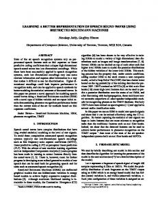
Figure 1: The graphical model used in Factored Latent Analysis (FLA).
p(X(t), O(t)) = p(X(t)|O(t))p(O(t)) Our model and estimation is different in two respects. First, we explicitly factored the observations as shown in Figure 1. This results in a separate latent class model for each of a number of different descriptions allowing direction, speed, size, and location to have completely independent descriptions. Second, we estimate the model using pairwise observation statistics. Stauffer and Grimson [6] built hierarchical models using pairwise joint co-occurrence of observations of a single type. This work is similar, but uses all the pairwise observation between different characteristics to induce latent class models that are consistent with those statistics across multiple aspects.
(1)
where p(O(t)) is the probably of being in a particular state and p(X(t)|O(t)) is the conditional likelihood of producing a particular set of observations. In this work we assume that X(t) and O(t) reflect only aspects of the object which are observable. Figure 1 shows the graphical model used in Factored Latent Analysis. In the model, the observed state X(t) is factored into K separate variables, (X1 (t), X2 (t), ..., XK (t)), and each variable is represented by its own latent variable. We assume that the ith observation Xi (t) can be drawn independently from a distribution conditioned on the latent variable Li . This is the latent class conditional output distribution p(Xi |Li ). An instance of this variable can have one of ki possible values, each representing a latent class. For instance, observations of normalized size Xs (t) ideally would be a single value with additive noise. In an environment with people, cars, and trucks, a coarse approximation would be three latent size classes, or ls ∈ {0, 1, 2}. Conditioned on its latent class, an object should exhibit a particular size with additive measurement noise. In reality, there may be multiple classes of pedestrian and vehicle sizes, which may suggest a hierarchical approach. Observations of normalized velocity Xv (t) in a particular environment may be well-represented by three latent classes: stopped, walking, jogging. Determining the ”correct” number of classes for each latent variable ki is a difficult problem that is not fully addressed in this work. Our approximation to p(O(t)) is a multinomial distribution over every possible combination or latent class labels, or p(l1 , l2 , ..., lK ). For instance, a particular scene may have a high likelihood of observing small slow objects moving in any direction and large fast objects moving in one of two primary directions and a very low likelihood of observing all other possible object states. Thus, based on the independence assumptions in this
Many varieties of data-driven perceptual data mining[5] techniques have been applied to activity analysis. Johnson and Hogg [3] clustered trajectories in a scene into 400 representative clusters allowing generalization and prediction, but not compact description. Stauffer and Grimson [6] used a hierarchal clustering technique to develop a binary tree classification hierarchy, which is somewhat more compact but also not segmental. Because these approaches describe entire paths holistically it is unclear how they can be adapted to describe compound activities. Makris and Ellis[4] also clustered entire trajectories into independent paths, but they extracted common features of paths to describe way points enabling some segmentation of the entire sequence but still a limited description of each segment. This paper describes a method for learning an effective factored segmental description of activity in scenes directly from the tracking data using observed pairwise joint cooccurrences. Section 2 describes the statistical model. Section 3 discusses the estimation technique advocated by the graphical model. Section 4 describes an alternative approximate technique chosen for this work because of computational viability. Section 5 shows this model applied in multiple environments. Section 6 and Section 7 discuss future work and conclusions that can be drawn from this work. 2
model, equation 1 becomes p(x1 , x2 , ..., xK ) =
�
p(l1 , l2 , ..., lK )
K �
vectors observed. For a nominal number of latent classes (approximately 3 or 4) over a nominal number of observation types (3 or 4) over the number of observations in a single hour of tracking, a single EM iteration can take as much as 1 day. If the observations xi are kept continuous and are more complex than scalar values like velocity (for example, silhouettes or color histograms), each EM step could take weeks. For this reason, we present the alternative in the next section.
p(xi |li ),
i=1
(l1 ,l2 ,...lK )∈L
(2) where L is the set of all possible combinations of latent aspect assignments. Although many of the possible combinations will tend to have zero probability of occurring, the number of potential combinations is |L| =
K �
ki ,
4. Estimation from pairwise observation statistics
(3)
i=1
This section describes our approach to approximating the Factored Latent Analysis model as applied to the problem of activity analysis. It describes: quantization of the (potentially) continuous output observations; estimation of pairwise joint observation statistics; estimating the latent class likelihoods and mixing probabilities from the pairwise statistics; and classification using the model.
where ki is the number of latent classes for each type of observations. The number of latent classes for each observation, ki , is the primary means by which the capacity of this model is limited. In the examples in this work, this number has been chosen, but Section 6 discusses how this part of the estimation could be automated.
3. Estimation Techniques 4.1. Quantization of observation spaces
Given the form of the model and a large set of observations, it is possible to estimate the maximum likelihood parameters of the model. We raise two potential estimation techniques. Subsection 3.1 describes how the entire joint latent model could be estimated directly from the data. The potential advantages and pitfalls of this technique are outlined. Due to the type and quantity of data in the problem we are considering, a computationally feasible alternative is introduced in Section 4. This alternative is an approximate technique for estimating the model from aggregate observation statistics between pairs of different observation types.
Our first approximation is to discretize the output observations for each type of observation. This can be done by uniformly binning the output space or using vector quantization to more compactly represent the output space. Thus, potentially continuous observations, xi , can be represented by a discrete set of prototypical values x˙ i . Figure 2 shows a scene with overlayed tracking data. For this scene, we will make discretized measurements of size, velocity, direction, and position. In most cases, we will simply partition the measurements from their min to max value into equal sized bins. Using 64 bins to represent sizes, velocities, and directions is sufficent, whereas position is a two dimensional space requiring more bins. In theory, this quantization is not necessary, but it makes it computationally feasible to collect estimates of joint occurrences of observations of type i and type j, or pˆ(xi , xj ). The primary advantage is that the discretized joint occurrence estimate pˆ(x˙ i , x˙ j ) will remain a constant size regardless of the number of observations. Because there are potentially tens of thousands of tracked objects per hour and each tracked object can contain hundreds of valid temporal windows, this approximation is required to make this application computationally feasible.
3.1. Complete EM estimation The obvious approach to estimating the parameters of the model is a straight-forward EM implementation. The hidden variable is the latent class assignment. The E-step involves computing the likelihood over each latent variable given model of p(l1 , ..., lK ) and p(xi |li ). The M-step involves maximizing the model parameters given the latent likelihoods. The exact form of the model will dictate the complexity of both steps. For instance, p(xi |li ) could be a multinomial distribution, a Gaussian distribution, or a mixture of Gaussians and p(l1 , ..., lK ) could be a multinomial joint distribution with a uniform prior, a Dirichlet prior, or any other alternative. Using this approach, one can estimate the full joint distribution over the latent classes p(l1 , l2 , ..., lK ) using all the data while simultaneously estimating the class conditional output distributions p(xi |li ). Unfortunately, the computational complexity of this procedure is at least O(N k1 k2 ...kK ), where N is the number of observation
4.2. Estimating pairwise joint observations If one was provided segmented, labeled data for a particular observation type, the class conditional probabilities p(xi |li ) could be estimated directly. Unfortunately, our data is neither segmented nor labeled for any of the types of observations. 3
10
velocity (s)
20 30 40 50 60 10
20
30 40 size (v)
50
60
Figure 3: An example joint occurrence over size and velocity, or pˆ(x˙s , x˙v ), estimated from a scene containing pedestrians and vehicles. Brighter indicate higher likelihood of cooccurrences within a window of observations drawn from a single joint latent class.
Figure 2: This figure shows the traffic in a particular environment after rectification. Green circles denote beginnings of track and red x’s denote ends of tracks. A large portion of the traffic is on the roads in either primary direction. But pedestrians are often seen crossing the road and moving to or away from the office building on the right.
”size” is estimated as the square root of the number of pixels and ”velocity” refers to the speed an object is travelling in normalized coordinates after rectification. As is evident in the figure, there are two main types of objects: slow-moving small objects and fast-moving large objects. Although, it is interesting to note that both the small objects and the large objects can be observed in a stopped or loitering state. This estimate can be accumulated in an online fashion, as follows
Because we lack an oracle to segment the sequences for each observation type, we make an assumption that the observations within a temporal Gaussian weighted window are of the same latent class. This assumption is an integral part of this learning technique. For object activity, we use a window of one second duration. Within such a window an object’s size, velocity, direction of travel and location are assumed to be drawn independently from a single latent class for each observation type. For instance, over a single second a particular object could be described as a small, fastmoving object travelling north on the highway. This corresponds to one possible N-tuple joint latent state assignment in the set L. If the temporal window size is too small, a randomly chosen window would exhibit little within class variability in the observations. If the temporal window is too large, many randomly sampled windows would include observations drawn from multiple latent classes. pˆ(x˙ i , x˙ j ), is an estimate of the likelihood that a pair of observations of type i and type j would be drawn from a short temporal window. Given a large set of randomly sampled temporal windows that are primarily uniform in their underlying joint latent class, pˆ(x˙ i , x˙ j ) is a frequentist approximation to the true joint occurrence probability. Figure 3 shows pˆ(x˙s , x˙v ) for a scene containing pedestrians and vehicles, where xs is an observation of object size and xv is an observation of object velocity. In this case,
pˆ(x˙ i , x˙ j ) =
N �
wn pn (x˙ i , x˙ j ),
(4)
n=1
where pn (x˙ i , x˙ j ) is the joint cooccurrence within a particular window and wn is a weight for that window. Thus, the aggregate estimate and the sum of the weights are sufficient statistics. The weight can be used to decrease the affect of extremely redundant observed states. For instance, the weight for the hundreds of redundant observations of a car that stops in the scene for two minutes can be decreased to lessen their total effect on pˆ(x˙ i , x˙ j ).
4.3. Estimating pairwise latent class conditional and prior distributions Given an estimate of pˆ(x˙ i , x˙ j ) for pairs of observations of type i and type j and a number of latent size classes ks and number of latent velocity classes kv , it is possible to estimate the model parameters that best approximate those joint statistics. 4
size
ss
p(x |l )
s
l
size
l =0 s ls=1
l
size (s)
v
velocity direction
velocity (v)
velocity (v)
20
20
20
40
40
40
60
60
60
40
60
20
40
60
60 20
40
60
20406080100 120 140
20
20
20
20
40
40
40
40
60
60
60
40
60
20
40
60
60 20
40
60
20406080100 120 140
20
20
20
20
40
40
40
40
60
60
60
20
position
position
40
20
40
60
20 40 60 80 100 120 140
20
40
60
20 40 60 80 100 120 140 20
p(xv|lv)
direction
20
20
l =0 v lv=1 lv=2
velocity
40
60
60 20
40
60
20 40 60 80 100 120 140 20
40
60
20406080100 120 140 20 40 60 80 100 120 140
20
40
60
20406080100 120 140
size (s)
Figure 5: This figure shows 16 matrices corresponding to each possible pˆ(x˙ i , x˙ j ) for the scene shown in Figure 2 given a one second equivalency window.
Figure 4: This figure shows: the latent pair likelihoods, p˜(ls , lv ), on the upper left; the conditional likelihood models for each latent object size class, p˜(x˙ s |ls ), on the upper right; the conditional likelihood for each latent object velocity class, p˜(x˙ v |lv ), on the lower left; and the models implied joint statistics as outlined in Equation 5 on the lower right.
both classes are sometimes observed loitering for periods of time. Also, the loitering distribution captures the variance that is observed in loitering objects, because even a parked car will will exhibit some measurement noise in the observed location. This is an important feature when classifying sequences. While this process could be done independently for each possible pair of observations, it would result in multiple latent class models for each independent factor. E.g., two latent class models for size given velocity; two latent class models for size given direction; and so on. The next subsection describes how just K sets of latent models can be estimated that are consistent with K 2 pairwise joint estimates.
Given the model’s estimates of the mixing likelihoods p˜(ls , lv ), and conditional output likelihoods for p˜(x˙ s |ls ) and p˜(x˙ v |lv ) the likelihood of observing a particular pair of observations from the model is simply � p˜(ls , lv )˜ p(x˙ s |ls )˜ p(x˙ v |lv ), (5) p˜(x˙ i , x˙ j ) = (ls ,lv )∈Lsv
where Lsv is the set of all pair of latent size and velocity assignments. Given random initial estimates of p˜(ls , lv ), p˜(x˙ s |ls ), and p(x˙ v |lv ), the model parameters that maximize the likelihood of the data can be iteratively estimated using an EM procedure. This equates to minimizing the KL divergence between the joint statistics of the model p˜(x˙ i , x˙ j ) and the observed joint statistics pˆ(x˙ i , x˙ j ). Figure 4 shows the maximum likelihood model for the pˆ(x˙ i , x˙ j ) shown in Figure 3 after convergence. It is evident by comparing the two joints, that the model is able to effectively approximate the joint statistics with only two latent size classes and three latent velocity classes. The two latent size classes correspond to pedestrians and vehicles. The bimodal pedestrian class results from individual pedestrians and pairs of connected pedestrians. The three latent velocity classes roughly correspond to loitering, walking, and driving through the scene. As is evident in the mixing matrix, p˜(ls , lv ), on the upper left, most pedestrians walk, most vehicles drive, but
4.4. Exploiting K 2 pairwise joint observations In general, Factored Latent Analysis includes K sets of latent classes p˜(x˙ i |li ), one for each type of latent observation, and a model for drawing latent class combinations p˜(li , lj ). The goal of our method is to estimate the K sets of latent class models for each independent factor and the pairwise mixing proportions that best approximate all the pairwise observations. One can trivially estimate K 2 pairwise joint observation estimates1 , each of which corresponds to a possible pair of observation types. Figure 5 shows all pairwise joint observations for the scene shown in Figure 2. It is obvious that there is significant structure in these pairwise joint statistics. For instance, 1 Since p ˆ(x˙ i , x˙ j ) is redundant with pˆ(x˙ j , x˙ i ), only need to be stored.
5
K(K+1) 2
pairs
size
velocity
direction
position
size
size
size
velocity
velocity
direction
direction
20
20
20
40
40
40
60
60
60
40
60
20
40
60
60 20
40
60
20406080100 120 140
20
20
20
20
40
40
40
40
60
60
60
40
60
20
40
60
60 20
40
60
20406080100 120 140
20
20
20
20
40
40
40
40
60
60
60
20
position
position
40
20
position
direction
20
20
40
60
20 40 60 80 100 120 140
20
40
60
20 40 60 80 100 120 140 20
(a)
velocity
40
60
60 20
40
60
20 40 60 80 100 120 140 20
40
60
20406080100 120 140 20 40 60 80 100 120 140
20
40
60
20406080100 120 140
(b)
Figure 6: This figure shows latent classes and their mixing ratios (a) and the resulting p˜(x˙ i , x˙ j ). small objects tend to loiter or move slow. Large objects tend to move faster in one of two primary directions (north and south). Because of the 2D nature of position, it is difficult to interpret the last row and column without performing classification (see Section 5). Given a complete set of K latent class conditional output distributions p˜(x˙ i |li ) and K 2 pairwise latent marginal distributions p˜(li , lj ), every marginal pairwise output distribution p˜(x˙ i , x˙ j ) can be estimated. By minimizing the KL divergence between all of the pairwise output distributions and pairwise output estimates the likelihood of the data given the model can be maximized. The criterion is � d(ˆ p(x˙ i , x˙ j )||˜ p(x˙ i , x˙ j )), (6) θ˜∗ = argmin θ˜
to pedestrians and vehicles even though the distribution of pedestrian sizes is bimodal. This is due to the fact that pedestrians and pairs of pedestrians exhibit similar speeds, directions, and locations. The same velocity classes also occur. Using only the diagonal elements p˜(x˙ i , x˙ i ) of Figure 6(a), the likelihood of each latent class is evident. There are two common directions corresponding to the road directions. These directions are taken by both pedestrians and vehicles, but there are many directions that are only taken primarily by pedestrians. These results will be discussed further in Section 5 along with other examples.
4.5. Applying the model to classification While any state observation X(t) could be classified into one of each type of latent class independently, it is important to remember what the class conditional likelihoods actually represent. They were calculated based on an assumption of temporal coherency, thus the latent class likelihoods for a particular time t are estimated from more than simply X(t). Currently, we simply assume the latent class posteriors are the weighted expectation of the independent posterior estimates over the observations temporal coherency window. This performs smoothing which greatly reduces the number of spurious detections from instantaneous tracking glitches and short-term changes. In video surveillance, such spurious measurements can result from object interactions, shadow effects, lighting effects, and other tracking failures
i,j
where θ˜ is the parameters of the K sets of ki multinomials over |x˙ i | and the K 2 ki by kj latent joint distributions. This equates to maximizing the likelihood of all pairwise measurements. Figure 6 (a) shows the model parameters θ˜ and Figure (b) shows the corresponding p˜(x˙ i , x˙ j ) for the scene shown in Figure 2 after convergence. This model was automatically estimated given two, three, six, and eight latent classes respectively for size, velocity, direction, and position. Not surprisingly, many of the latent class conditional distributions have intuitive interpretations. As in the previous subsection, the latent size classes roughly correspond 6
and are extremely common.
will be more desirable to split vehicles into cars and trucks if they also exhibit different speed, direction, or location characteristics. Related to the issue of choosing the number of classes is learning class labels. In fact, labels given from an oracle could simply be another observation type. Finally, there are many more characteristics that can be included in this estimation. This could include average color, color histograms, shape, sparsity, internal object deformation, source location, or sink location. Each of these characteristics may bear new information on object activity, class, or appearance.
5. Results While the model learned in the previous section is intuitively pleasing, this section will show classification of specific tracking sequences and show how these provide an effective description of tracking sequences. Figure 7(a) shows a new set of tracked data from our previous scene. The latent classes from the unsupervised training are nearly identical to the example in the previous section despite differences in the number of objects or distributions of their behaviors. Figure 7 (b)-(e) show the maximum likelihood classification of the observation for hundreds of sequences. See the figure for a detailed description. These results illustrate how position latent classes tend to represent areas which contain similar types of object moving in similar ways. For example, in Figure 7(e) the blue class corresponds to an area where cars and pedestrians are present and both are likely to be in the ”loitering” state. Figure 8 and Figure 9 show results for two other environment with the same number of latent classes. See the figures for detailed description. Each example learned a set of classes for all four types of observations that are specific to a particular environment and input. In these two cases, the number of latent classes was arguably too large, but the clustering was still meaningful. By a simple process of labeling these latent classes with textual descriptions, interesting compound queries can be constructed. E.g., ”show me the pedestrians that crossed the road.” ”How many vehicles stopped in the loading zone?” ”How many individuals who stopped in the scene started in the opposite direction?” ”How much of the traffic on the road is vehicles?” ”Did anything stop in the scene for more than 30 seconds?” These queries illustrate the importance of factored representation and the ability to segment effectively.
7. Summary We have presented a method for approximating the Factored Latent Analysis model using pairwise joint observation estimates pˆ(x˙ i , x˙ j ). This factored model enables a compact description of object properties, which is more useful than many previous automatically-generated unfactored descriptions. Our model also enables tracking sequences to be segmented into component parts effectively. This is essential in describing compound activities that occur in most environments. This algorithm exhibited good performance across many environments by exploiting the pairwise observations and temporal coherence. We believe this work shows promise and intend to pursue further related avenues of research.
References [1] D. M. Blei, A. Y Ng, and M. I. Jordan. Latent dirichlet allocation. In Journal of Machine Learning Research, volume 3(4), pages 993–1022, 2003. [2] Thomas Hofmann. Probabilistic latent semantic analysis. Proceedings of the Fifteenth Conference on Uncertainty in Artificial Intelligence (UAI’99), 1999. [3] Neil Johnson and David Hogg. Learning the distribution of object trajectories for event recognition. In British Machine Vision Conference, volume 2, pages 583–592, September 1995.
6. Future Work We look forward to implementing an efficient estimation technique for estimation of the complete p(l1 , l2 , ..., lK ) as described in Section 2. This would have a number of advantages. Rather than having estimates of all pairwise latent joints p˜(li , lj ), we would have the full latent joint distribution, p˜(l1 , l2 , ..., lK ). Another major issue is choosing the ”correct” number of latent classes for each observation type. We intend to implement a model selection criteria based on the Bayesian Information Criterion, which will incorporate a measure of the mutual information in the latent joint distribution. This will make splitting a latent class for one type of observation undesirable if it does not increase the information about other types of observations. For example with latent size, it
[4] Dimitrios Makris and Tim Ellis. Finding paths in video sequences. In British Machine Vision Conference, volume 1, pages 253–272, Manchester, UK, September 10-13 2001. [5] Chris Stauffer. Perceptual Data Mining. Phd dissertation, Massachusetts Institute of Technology, Artificial Intelligence Laboratory, June 2002. [6] Chris Stauffer and W. E. L. Grimson. Adaptive background mixture models for real-time tracking. In Computer Vision and Pattern Recognition, pages 246–252, 1999.
7
(a)
(b)
(c)
(d)
(e)
Figure 7: This figure shows a new set of tracked objects for the previously introduced scene as well as the classification of individual object states in each of the four latent class types. The latent size classes show that vehicles tend to be on the road or in the drop-off region. The latent velocity classes show that only the vehicles passing through on the north-south road travel faster than the nominal speed. Interestingly, there are some examples of pedestrian sized objects going the faster speed in the road region (bicycles and rollerbladers). Figure 7(d) shows north (orange) and south (blue) classes as well as traffic moving towards the office from the south (cyan) and from the north (yellow) and traffic moving away from the office (red). Figure 7(e) shows regions with similar characteristics. The road (dark blue) is a region unto itself. The sidewalk along the street on the north and south side of the scene (light blue) is split by either walking through the drop-off zone (blue) or through the angled sidewalks (orange and red).
(a)
(b)
(c)
(d)
(e)
Figure 8: This figure shows tracked data for pedestrians in a courtyard (a) and each observation classified in each of the four latent class models. The latent sizes primarily result from occluded and unoccluded pedestrians. Three pedestrians jogged away from the building and four pedestrians stopped. The stopping zones were clustered together (red) as were the major lanes of movement. There are north, south, east, west, northwest and southeast directions.
(a)
(b)
(c)
(d)
(e)
Figure 9: This figure shows tracked data for a indoor, mid-field scene with pedestrians. Again, the size classes correspond to occluded humans. The two major directions of travel (orange and cyan) correspond to most of the traffic. The red and blue regions were areas in the scene where pedestrians stopped.
8