with other states depends on the specific DAG of the equivalence class, so the best transition might not be performed if
Learning a L1-regularized Gaussian Bayesian network in the space of equivalence classes
Diego Vidaurre
[email protected] Concha Bielza
[email protected] Pedro Larra˜ naga
[email protected] Departamento de Inteligencia Artificial. Universidad Polit´ecnica de Madrid,Campus de Montegancedo s/n, Spain Keywords: Gaussian networks, model selection, regularization, Lasso, learning from data, equivalence classes
Abstract Learning the structure of a graphical model from data is a common task in a wide range of practical applications. In this paper we focus on Gaussian Bayesian networks (GBN), that is, on continuous data and directed graphs. We propose to work in an equivalence class search space that, combined with regularization techniques to guide the search of the structure, allows to learn a sparse network close to the one that generated the data.
1. Introduction In a GBN, we have a joint Gaussian probability distribution on a finite set of variables. Each variable Xi has its own univariate normal distribution given its parents. The relationships between the variables are always directed. The joint probability distribution is built on the product of the distributions of each Xi . There are two basic approaches for structure learning: independence tests and score+search methods. A popular score+search procedure is based on greedy methods, where a score function and a neighbourhood have to be defined. To represent the solutions and move in the search space, we typically choose between directed acyclic graphs (DAGs) or partial directed acyclic graphs (PDAGs). An equivalence class, modelled by a PDAG, is the set of graphs that encodes a unique probability distribution with the same conditional independences. It is often the preferred representation and the only one capable to fit the inclusion boundary (IB) requirement (Chickering, 2002). Appearing in Proceedings of the 25 th International Conference on Machine Learning, Helsinki, Finland, 2008. Copyright 2008 by the author(s)/owner(s).
Three main problems arise when working in the DAG space rather than with equivalence classes. First, some operators defined to move between DAGs may operate between graphs in the same equivalence class, being a useless waste of time. Second, a random factor is introduced: the connectivity of the current real state with other states depends on the specific DAG of the equivalence class, so the best transition might not be performed if equivalence classes are ignored. Given that all members of a class score the same value, there is no reason other than randomness to prefer a specific member. The third problem is related to the a priori probability that the final DAG belongs to a specific equivalence class. If all DAGs in the same class are interpreted as different models, the a priori probability of an equivalence class to be the final output is the sum of the a priori probabilities of each DAG inside it. It has consequences that are difficult to be predicted. A model is defined to be inclusion optimal with regard to a distribution p(X1 , ..., Xn ) if it includes p(X1 , ..., Xn ) and there is not any model strictly included in the model that includes p(X1 , ..., Xn ). It is well-known that a greedy algorithm that respects the IB neighbourhood and uses a locally consistent scoring criterion is asymptotically optimal under the faithful assumption, and inclusion optimal under the weaker composition property assumption (Chickering & Meek, 2002). This is the case of the greedy equivalence search algorithm (GES) developed in (Chickering, 2002). As a generalization of algorithm GES, (Nielsen et al., 2003) implement the KES algorithm –k-greedy equivalence search– for Bayesian network learning, where a stochastic factor is introduced so that multiple runs can be made to extract common patterns on the solutions, that is, to include in the final model just those arcs that showed up in most of the runs. For simplicity, we will not work with several
Learning a L1-regularized Gaussian Bayesian network in the space of equivalence classes
runs and extraction of common patterns. Here, we extend the KES algorithm to continuous (Gaussian) distributions and learn sparser models based on regularization techniques, specifically on the least absolute shrinkage and selection operator, commonly named Lasso (Tibshirani, 1996). The main idea, previous to the learning stage in the equivalence class space, is to use Lasso for each variable X on the remaining variables, discarding as possible parents of X in the GBN those variables whose coefficients become zero so as to reach simple models that properly fit available data. To reduce the computational burden, we also take advantage of the convexity of the score for each separate variable against the rest of them.
2. KES combined with Lasso As noted in (Nielsen et al., 2003), we may relax the greediness of GES algorithm in such a way that optimality is still reached under the conditions exposed above. Stochastic equivalence search algorithm (SES) does a trade-off between randomness and greediness, selecting at each step any of the models that improve the score. KES is the generalization of these algorithms, allowing the user to set the degree of randomness via a parameter 0 ≤ k ≤ 1, and keeping asymptotical optimality under these conditions. Being the IB neighbourhood the union of the lower and upper IB, that is, those models whose set of conditional independences constraints immediately precedes (is contained) or follows (contains) the current model, KES selects at each step the best model from a random set which size is a ratio k of all the models in the IB neighbourhood that improve the score. We are using GES if we set k = 1, and SES for k = 0. Note that, although SES asymptotically finds with probability greater than zero any inclusion optimal model, and hence it visits this best model when running enough times, the number of inclusion optimal models is exponential with regard to the number of variables. Therefore, when there are many, the search space becomes huge and an optimal solution is difficult to be found. At this point is where L1-regularization (Lasso) comes into play, because of its ability to make coefficients of irrelevant variables be zero. The Lasso (Tibshirani, 1996) uses least-squares regression with L1-regularization, adding a penalty term that leads the sum of the absolute values of the coefficients to be small. Its weight is controlled by parameter λ: The larger the λ is, the stronger its influence and the smaller the number of variables. (Wainwright et al., 2006) show interesting theoretical properties of L1regularization, proving the consistency of the method
Algorithm 1 KES plus Lasso Input: data set with n variables, k ∈ [0, 1] Output: partially directed acyclic graph G for i = 1 to n do Calculate L1-regularization path of variable Xi P otentialP arents(i) := set of variables in path with best MDL score end for Initialize G := Empty or randomly generated model repeat K := size(IB(G, P otentialP arents)) ∗ k where IB(G, P otentialP arents) is the IB(G) constrained by Lasso S := set of K models drawn from IB(G, P otentialP arents) G′ := the model from S with the best MDL score if M DL(G′ ) < M DL(G) then G := G′ end if until noChange is true
when both the number of nodes and the maximum number of parents per variable are under the limit marked by a function of the number of observations. Based on Lasso, we propose a previous step to preselect a set of potential parents for each variable, on which the KES algorithm will work greedily. Pseudocode is shown in Algorithm 1. In (Schmidt et al., 2007) a similar approach using a DAG search space is proposed with very good results. As noted in this work, not all the nodes should share the same value of λ in its corresponding Lasso. A common strategy to select λ is to choose it using cross-validation, introducing heavy computational load. For this reason, they suggest to find the best (score equivalent) MDL score λ. Since the number of variables with non-zero coefficients is piecewise constant, and only grows at specific values of λ, we just need to find the best λ from a finite set of values. Note that the set of Lasso weights, solved via the least angle regression algorithm (LARS) (Efron et al., 2004), is different from the parameters of the GBN that will be learnt in the second phase, and are only used to discard parents in the greedy algorithm. Moreover, this paper introduces a simple improvement on the LARS algorithm when used for the GBN learning. Given a variable, the MDL score over the remaining other variables follows a convex curve along the regularization path, with only one local minimum. Thus, we may stop the LARS algorithm in a very early phase, so that we do not need to calculate the whole regularization path. In addition, this local minimum is often reached at the beginning of the regularization
Learning a L1-regularized Gaussian Bayesian network in the space of equivalence classes
path, saving a great deal of computational cost. Restricting to this previous subset of potential parents does not make the KES algorithm to lose the theoretical properties that we described above if we assume L1-regularization to be an ideal variable selector. In this case, it is guaranteed to find a set of variables with all the parents, children and co-parents (the Markov blanket). Hence, Lasso is only discarding false parents. As well as (Nielsen et al., 2003) do, we do not calculate the complete IB neighbourhood at each step. We rather approximate its size (taking the Lasso restriction into account) and derive a k-proportion of it. Thus, we are not actually drawing a k-proportion from the set of models that are better than the current one, but an approximate k-proportion from the total, keeping the best one.
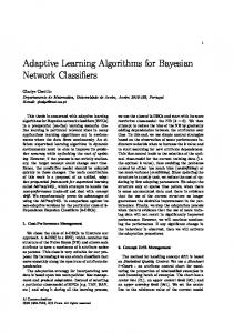
information makes the output network to be sparser and tends to include less false arcs, while the amount of true arcs is not very different from the ones found without the Lasso information. We also observe that intermediate values of k, that is, moderate randomness, result in slightly better networks when Lasso is not used. When using Lasso, this tendency is negligible: with the Lasso pre-selection phase, the algorithm becomes somewhat robust to k, which is actually an advantage. In addition, the computational cost is orders of magnitude underneath. Moreover, when we use early stop in the Lasso algorithm we are saving around 65.5% of computation time in this first phase. As future work, we plan to study the effect of executing multiple runs so as to induce common features in the networks obtained, and apply it to more complex data.
Acknowledgments
3. Experiments The Alarm network1 contains 37 nodes and 46 arcs and is commonly used to test learning algorithms of Bayesian networks. We will use its dependencies to simulate continuous data sets of 1000 samples. The parameters of the distribution are generated at random. We run the KES algorithm for 10 different values of k : 0.1, 0.2, ..., 0.9, 1.0, using a previous Lasso step and without using it. For each k, we performed 10 runs and calculated the mean and standard deviation of each experiment. Results are shown in Figure 1.
90
Research partially supported by the Spanish Ministry of Education and Science, project TIN2007-62626. Thanks also to Jens Nielsen for valuable support
References Chickering, D. M. (2002). Optimal structure identification with greedy search. Machine Learning, 3, 507–554. Chickering, D. M., & Meek, C. (2002). Finding optimal bayesian networks. Proceedings of the International Conference on Uncertainty in Artificial Intelligence (pp. 94–102).
80 70 60 Arcs
50
F. positives
40
Matches
30 20
Nielsen, J., Kocka, T., & Pe˜ na, J. (2003). On local optima in learning Bayesian networks. Proceedings of the International Conference on Uncertainty in Artificial Intelligence (pp. 435–442).
10 0 k0.1 k0.2 k0.3 k0.4 k0.5 k0.6 k0.7 k0.8 k0.9 k1.0
90 80 70 60 Arcs
50
F. positives
40
Efron, B., Johnstone, I., Hastie, T., & Tibshirani, R. (2004). Least angle regression. Annals of Statistics, 32(2), 407–499.
Matches
30 20 10 0 k0.1 k0.2 k0.3 k0.4 k0.5 k0.6 k0.7 k0.8 k0.9 k1.0
Figure 1. KES algorithm without (top) and with (bottom) Lasso parents preselection.
The main conclusion to be drawn is that the Lasso 1 http://compbio.cs.huji.ac.il/Repository/ Datasets/alarm/alarm.htm
Schmidt, M. W., Niculescu-Mizil, A., & Murphy, K. P. (2007). Learning graphical model structure using L1-regularization paths. Proceedings of the Association for the Advancement of Artificial Intelligence AAAI (pp. 1278–1283). Tibshirani, R. (1996). Regression shrinkage and selection via the lasso. Journal of the Royal Statistical Society. Series B, 58, 267–288. Wainwright, M., Ravikumar, P., & Lafferty, J. (2006). Inferring graphical model structure using L1-regularized pseudo-likelihood. NIPS.