However, they tend to perform poorly when learned in the standard way. This is
at- tributable to a mismatch between the objec- tive function used (likelihood or a
...
Learning Bayesian Network Classifiers by Maximizing Conditional Likelihood
Daniel Grossman
[email protected] Pedro Domingos
[email protected] Department of Computer Science and Engineeering, University of Washington, Seattle, WA 98195-2350, USA
Abstract Bayesian networks are a powerful probabilistic representation, and their use for classification has received considerable attention. However, they tend to perform poorly when learned in the standard way. This is attributable to a mismatch between the objective function used (likelihood or a function thereof) and the goal of classification (maximizing accuracy or conditional likelihood). Unfortunately, the computational cost of optimizing structure and parameters for conditional likelihood is prohibitive. In this paper we show that a simple approximation— choosing structures by maximizing conditional likelihood while setting parameters by maximum likelihood—yields good results. On a large suite of benchmark datasets, this approach produces better class probability estimates than naive Bayes, TAN, and generatively-trained Bayesian networks.
1. Introduction The simplicity and surprisingly high accuracy of the naive Bayes classifier have led to its wide use, and to many attempts to extend it (Domingos & Pazzani, 1997). In particular, naive Bayes is a special case of a Bayesian network, and learning the structure and parameters of an unrestricted Bayesian network would appear to be a logical means of improvement. However, Friedman et al. (1997) found that naive Bayes easily outperforms such unrestricted Bayesian network classifiers on a large sample of benchmark datasets. Their explanation was that the scoring functions used in standard Bayesian network learning attempt to opAppearing in Proceedings of the 21 st International Conference on Machine Learning, Banff, Canada, 2004. Copyright 2004 by the authors.
timize the likelihood of the entire data, rather than just the conditional likelihood of the class given the attributes. Such scoring results in suboptimal choices during the search process whenever the two functions favor differing changes to the network. The natural solution would then be to use conditional likelihood as the objective function. Unfortunately, Friedman et al. observed that, while maximum likelihood parameters can be efficiently computed in closed form, this is not true of conditional likelihood. The latter must be optimized using numerical methods, and doing so at each search step would be prohibitively expensive. Friedman et al. thus abandoned this avenue, leaving the investigation of possible heuristic alternatives to it as an important direction for future research. In this paper, we show that the simple heuristic of setting the parameters by maximum likelihood while choosing the structure by conditional likelihood is accurate and efficient. Friedman et al. chose instead to extend naive Bayes by allowing a slightly less restricted structure (one parent per variable in addition to the class) while still optimizing likelihood. They showed that TAN, the resulting algorithm, was indeed more accurate than naive Bayes on benchmark datasets. We compare our algorithm to TAN and naive Bayes on the same datasets, and show that it outperforms both in the accuracy of class probability estimates, while outperforming naive Bayes and tying TAN in classification error. If the structure is fixed in advance, computing the maximum conditional likelihood parameters by gradient descent should be computationally feasible, and Greiner and Zhou (2002) have shown with their ELR algorithm that it is indeed beneficial. They leave optimization of the structure as an important direction for future work, and that is what we accomplish in this paper. Perhaps the most important reason to seek an improved Bayesian network classifier is that, for many
applications, high accuracy in class predictions is not enough; accurate estimates of class probabilities are also desirable. For example, we may wish to rank cases by probability of class membership (Provost & Domingos, 2003), or the costs associated with incorrect predictions may be variable and not known precisely at learning time (Provost & Fawcett, 2001). In this case, knowing the class probabilities allows the learner to make optimal decisions at classification time, whatever the misclassification costs (Duda & Hart, 1973). More generally, a classifier is often only one part of a larger decision process, and outputting accurate class probabilities increases its utility to the process. We begin by reviewing the essentials of learning Bayesian networks. We then present our algorithm, followed by experimental results and their interpretation. The paper concludes with a discussion of related and future work.
2. Bayesian Networks A Bayesian network (Pearl, 1988) encodes the joint probability distribution of a set of v variables, {x1 , . . . , xv }, as a directed acyclic graph and a set of conditional probability tables (CPTs). (In this paper we assume all variables are discrete, or have been prediscretized.) Each node corresponds to a variable, and the CPT associated with it contains the probability of each state of the variable given every possible combination of states of its parents. The set of parents of xi , denoted πi , is the set of nodes with an arc to xi in the graph. The structure of the network encodes the assertion that each node is conditionally independent of its non-descendants given its parents. Thus the probability of an arbitraryQ event X = (x1 , . . . , xv ) can be comv puted as P (X) = i=1 P (xi |πi ). In general, encoding the joint distribution of a set of v discrete variables requires space exponential in v; Bayesian networks reduce this to space exponential in maxi∈{1,...,v} |πi |. 2.1. Learning Bayesian Networks Given an i.i.d. training set D = {X1 , . . . , Xd , . . . , Xn }, where Xd = (xd,1 , . . . , xd,v ), the goal of learning is to find the Bayesian network that best represents the joint distribution P (xd,1 , . . . , xd,v ). One approach is to find the network B that maximizes the likelihood of the data or (more conveniently) its logarithm: LL(B|D) =
n X d=1
log PB (Xd ) =
n X v X
log PB (xd,i |πd,i )
d=1 i=1
(1) When the structure of the network is known, this reduces to estimating pijk , the probability that variable i
is in state k given that its parents are in state j, for all i, j, k. When there are no examples with missing values in the training set and we assume parameter independence, the maximum likelihood estimates are simply the observed frequency estimates pˆijk = nijk /nij , where nijk is the number of occurrences in the training set of the kth state of xi with the jth state of its parents, and nij is the sum of nijk over all k. In this paper we assume no missing data throughout, and focus on the problem of learning network structure. Chow and Liu (1968) provide an efficient algorithm for the special case where each variable has only one parent. Solution methods for the general (intractable) case fall into two main classes: independence tests (Spirtes et al., 1993) and searchbased methods (Cooper & Herskovits, 1992; Heckerman et al., 1995). The latter are probably the most widely used, and we focus on them in this paper. We assume throughout that hill-climbing search is used; this was found by Heckerman et al. to yield the best combination of accuracy and efficiency. Hill-climbing starts with an initial network, which can be empty, random, or constructed from expert knowledge. At each search step, it creates all legal variations of the current network obtainable by adding, deleting, or reversing any single arc, and scores these variations. The best variation becomes the new current network, and the process repeats until no variation improves the score. Since on average adding an arc never decreases likelihood on the training data, using the log likelihood as the scoring function can lead to severe overfitting. This problem can be overcome in a number of ways. The simplest one, which is often surprisingly effective, is to limit the number of parents a variable can have. Another alternative is to add a complexity penalty to the log-likelihood. For example, the MDL method (Lam & Bacchus, 1994) minimizes M DL(B|D) = 21 m log n − LL(S|D), where m is the number of parameters in the network. In both these approaches, the parameters of each candidate network are set by maximum likelihood, as in the known-structure case. Finally, the full Bayesian approach (Cooper & Herskovits, 1992; Heckerman et al., 1995) maximizes the Bayesian Dirichlet (BD) score P (BS , D) = P (BS )P (D|BS ) qi ri v Y Y Y Γ(n0ijk + nijk ) Γ(n0ij ) = P (BS ) Γ(n0ij + nij ) Γ(n0ijk ) i=1 j=1 k=1
(2) where BS is the structure of network B, Γ() is the gamma function, qi is the number of states of the
Cartesian product of xi ’s parents, and ri is the number of states of xi . P (BS ) is the prior probability of the structure, which Heckerman et al. set to an exponentially decreasing function of the number of differing arcs between BS and the initial (prior) network. Each multinomial distribution for xi given a state of its parents has an associated Dirichlet P iprior0 distribution with parameters n0ijk , with n0ij = rk=1 nijk . These parameters can be thought of as equivalent to seeing n0ijk occurrences of the corresponding states in advance of the training examples. In this approach, the network parameters are not set to specific values; rather, their entire posterior distribution is implicitly maintained and used. The BD score is the result of integrating over this distribution. See Heckerman (1999) for a more detailed introduction to learning Bayesian networks. 2.2. Bayesian Network Classifiers The goal of classification is to correctly predict the value of a designated discrete class variable y = xv given a vector of predictors or attributes (x1 , . . . , xv−1 ). If the performance measure is accuracy (i.e., the fraction of correct predictions made on a test sample), the optimal prediction for (x1 , . . . , xv−1 ) is the class that maximizes P (y|x1 , . . . , xv−1 ) (Duda & Hart, 1973). If we have a Bayesian network for (x1 , . . . , xv ), these probabilities can be computed by inference over it. In particular, the naive Bayes classifier is a Bayesian network where the class has no parents and each attribute has the class as its sole parent. Friedman et al.’s (1997) TAN algorithm uses a variant of the Chow and Liu (1968) method to produce a network where each variable has one other parent in addition to the class. More generally, a Bayesian network learned using any of the methods described above can be used as a classifier. All of these are generative models in the sense that they are learned by maximizing the log likelihood of the entire data being generated by the model, LL(B|D), or a related function. However, for classification purposes only the conditional log likelihood CLL(B|D) of the class given the attributes is relevant, where CLL(B|D) =
n X d=1
log PB (yd |xd,1 , . . . , xd,v−1 ).
(3)
Pn Notice LL(B|D) = CLL(B|D) + d=1 log PB (xd,1 , . . . , xd,v−1 ). Maximizing LL(B|D) can lead to underperforming classifiers, particularly since in practice the contribution of CLL(B|D) is likely to be swamped by the generally much larger (in absolute value) log PB (xd,1 , . . . , xd,v−1 ) term. A better approach would presumably be to use
CLL(B|D) by itself as the objective function. This would be a form of discriminative learning, because it would focus on correctly discriminating between classes. The problem with this approach is that, Pn unlike LL(B|D) (Equation 1), CLL(B|D) = d=1 log[PB (xd,1 , . . . , xd,v−1 , y)/PB (xd,1 , . . . , xd,v−1 )] does not decompose into a separate term for each variable, and as a result there is no known closed form for the optimal parameter estimates. When the structure is known, locally optimal estimates can be found by a numeric method such as conjugate gradient with line search (Press et al., 1992), and this is what Greiner and Zhou’s (2002) ELR algorithm does. When the structure is unknown, a new gradient descent is required for each candidate network at each search step. The computational cost of this is presumably prohibitive. In this paper we verify this, and propose and evaluate a simple alternative: using conditional likelihood to guide structure search, while approximating parameters by their maximum likelihood estimates.
3. The BNC Algorithm We now introduce BNC, an algorithm for learning the structure of a Bayesian network classifier by maximizing conditional likelihood. BNC is similar to the hillclimbing algorithm of Heckerman et al. (1995), except that it uses the conditional log likelihood of the class as the primary objective function. BNC starts from an empty network, and at each step considers adding each possible new arc (i.e., all those that do not create cycles) and deleting or reversing each current arc. BNC pre-discretizes continuous values and ignores missing values in the same way that TAN (Friedman et al., 1997) does. We consider two versions of BNC. The first, BNC-nP, avoids overfitting by limiting its networks to a maximum of n parents per variable. Parameters in each network are set to their maximum likelihood values. (In contrast, full optimization of both structure and parameters, described more fully in Section 4, would set the parameters to their maximum conditional likelihood values.) The network is then scored using the conditional log likelihood CLL(B|D) (Equation 3). The rationale for this approach is that computing maximum likelihood parameter estimates is extremely fast, and, for an optimal structure, they are asymptotically equivalent to the maximum conditional likelihood ones (Friedman et al., 1997). The second version, BNC-MDL, is the same as BNCnP, except that instead of limiting the number of parents, the scoring function CM DL(B|D) = 21 m log n −
CLL(S|D) is used, where m is the number of parameters in the network and n is the training set size. The goal of BNC is to produce accurate class probability estimates. If correct class predictions are all that is required, a Bayesian network classifier could in principle be learned simply by using the training-set accuracy as the objective function (together with some overfitting avoidance scheme). While trying this is an interesting item for future work, we note that even in this case the conditional likelihood may be preferable, because it is a more informative and more smoothlyvarying measure, potentially leading to an easier optimization problem.
4. Experiments To gauge the performance of our BNC variants for the task of classification, we evaluated them and several alternative learning methods on the 25 benchmark datasets used by Friedman et al. (1997). These include 23 datasets from the UCI repository (Blake & Merz, 2000) and 2 extra datasets developed by Kohavi and John (1997) for feature selection experiments. We used the same experimental procedure as Friedman et al., choosing either 5-fold cross-validation or holdout testing for each domain by the same criteria. In all cases, we measured both the conditional log likelihood (CLL) of the test data given the learned model, and the model’s classification error rate (ERR).
we used only 200 randomly-chosen samples for gradient descent, keeping the full training set to score networks and to fit the final parameters. This makes the running time of gradient descent independent of the training set size, while degrading the optimization only by increasing the variance of the objective function. Second, we imposed a maximum number of line searches for the gradient descent on each network. This takes advantage of the fact that the greatest improvement in the objective function is often obtained in the first few iterations. These alterations sped up the full optimization approach to the point where small domains (i.e., those with few attributes) such as core, diabetes, and shuttle-small, could be completed within an hour or two. Medium-sized domains (e.g., heart, cleve, breast) required on the order of five hours runtime. One of the larger domains, segment, was tried on a 2.4 GHz machine and was still running two days later when we terminated the process. The completed experiments revealed that neither the full optimization nor the accelerated versions produced better results than those obtained by BNC. We thus conclude that, at least for small to medium datasets, full optimization is unlikely to be worth the computational cost. 4.2. Structure Optimization We compared BNC with the following algorithms:
4.1. Full Structure and Parameter Optimization
• C4.5, for which we obtain only classification error results.
We first compared BNC to optimizing both structure and parameters for conditional log likelihood, to the extent possible given the computational resources available. In this version, the parameters of each alternative network at each search step are set to their (locally) maximum conditional likelihood values by the conjugate gradient method with line search, as in Greiner and Zhou (2002). The parameters are first initialized to their maximum likelihood values, and the best stopping point for the gradient descent is then found by two-fold cross-validation (this is necessary to prevent overfitting of the parameters).
• The naive Bayes classifier (NB).
Clearly, examining hundreds of networks per search step and performing gradient descent over all of the training data for each structure is impractical. For the smallest datasets in our experiments, full optimization was possible but took two orders of magnitude longer to complete than BNC (which requires several minutes on a 1 GHz Pentium 3 processor). To experiment on larger datasets, we introduced two variations. First,
• The tree-augmented naive Bayes (TAN) algorithm from Friedman et al. (1997). • HGC, the original Bayesian network structure search algorithm from Heckerman et al. (1995) that utilizes the Bayesian Dirichlet (BD) score (with Dirichlet parameters n0ijk = 1 and structure prior parameter κ = 0.1). • Two basic maximum likelihood learners, one using the MDL score (ML-MDL) and the other restricted to a maximum of two parents per node (ML-2P). We also tried higher maximum numbers of parents, but these did not produce better results. • NB-ELR and TAN-ELR, NB and TAN with parameters optimized for conditional log likelihood as in Greiner and Zhou (2002).
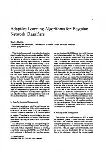
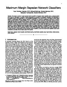
Mean negative-CLL and ERR data from BNC and the competing algorithms are presented in Tables 1 and 2, respectively. One-standard-deviation bars for those data points appear in the corresponding graphs in Figures 1 and 2. In both figures, points above the y = x diagonal are datasets for which BNC achieved better results than the competing algorithm. The significance values we report for these results below were obtained using the Wilcoxon paired-sample signed-ranks test.
(2002) observation that parameter optimization is less helpful for structures that are closer to the “true” one, and further supports the use of BNC. An additional advantage of BNC relative to ELR is that optimizing structure is arguably preferable to optimizing parameters, in that the networks it produces may give a human viewer more insight into the domain. Maximum likelihood parameters are also much more interpretable than conditional likelihood ones.
We also compared different versions of BNC. As with ML-2P, we found that increasing the maximum number of parents per node in BNC-nP did not yield improved results beyond the two-parent version. BNC2P outperformed BNC-MDL at the p < .01 and p < .001 significance levels for CLL and ERR, respectively. A similar comparison showed that ML2P likewise outperforms ML-MDL in both measures. These observations suggest that the MDL penalty is not well suited to the task of training Bayesian network classifiers, a conclusion consistent with previous results (e.g., Chickering and Heckerman (1997), Allen and Greiner (2000)) showing that MDL does not perform well for learning Bayesian networks. We thus used BNC-2P as the default version for comparison with other algorithms.
We suspect that there may be further performance differences between BNC and other algorithms that the benchmark datasets used in these experiments are too small and simple to elicit. For example, the advantage of discriminative over generative training should be larger in domains with a large number of attributes, and/or when the dependency structure of the domain is too complex to capture empirically given the available data. Conducting experiments in such domains is thus a key area for future research.
We see in Figures 1a and 2a that BNC-2P outperforms NB on both classification error (p < .06) and CLL (p < .001). BNC-2P and TAN have similar error rates (Figure 2b), but BNC outperforms TAN in conditional likelihood with significance p < .06 (Figure 1b). On these 25 datasets, NB performs about as well as C4.5 in terms of classification error. TAN, originally suggested as a superior alternative to C4.5 (Friedman et al., 1997), attained a significance level of only p < .24 against it in our experiments, whereas BNC-2P fared slightly better with p < .20. HGC, Heckerman et al.’s (1995) algorithm for learning unrestricted Bayesian networks, falls well below BNC in both the CLL and ERR metrics (p < .015, p < .006) (Figures 1c and 2c). As mentioned above, ML-MDL substantially underperforms other algorithms. ML-2P (Figures 1d and 2d) is competitive with BNC-2P in terms of conditional log likelihood, but BNC-2P outperforms it in classification accuracy in a large majority of the domains (p < .069). Finally, in Figures 1e,f and 2e,f we see that BNC-2P outperformed NB-ELR and TAN-ELR in CLL, while obtaining similar error rates. We also applied ELR optimization to the networks produced by BNC-2P. In all domains, ELR either converged to the original maximum likelihood parameters or to worse-performing ones. This is consistent with Greiner and Zhou’s
5. Related Work The issue of discriminative vs. generative learning has received considerable attention in recent years (e.g., Rubinstein and Hastie (1997)). It is now well understood that, although in the infinite-data limit an unrestricted maximum-likelihood learner is necessarily optimal, at finite sample sizes discriminative training is often preferable (Vapnik, 1998). As a result, there has been considerable work developing discriminative learning algorithms for probabilistic representations (e.g., the conditional EM algorithm (Jebara & Pentland, 1999) and maximum entropy discrimination (Jaakkola et al., 1999)). This paper falls into this line of research. Ng and Jordan (2002) show that, for very small sample sizes, generatively trained naive Bayes classifiers can outperform discriminatively trained ones. This is consistent with the fact that, for the same representation, discriminative training has lower bias and higher variance than generative training, and the variance term dominates at small sample sizes (Domingos & Pazzani, 1997; Friedman, 1997). For the dataset sizes typically found in practice, however, their results, ours, and those of Greiner and Zhou (2002) all support the choice of discriminative training. Discriminatively-trained naive Bayes classifiers are known in the statistical literature as logistic regression (Agresti, 1990). Our work can thus be viewed as an extension of the latter to include structure learning. Discriminative learning of Bayesian network structure has received some attention in the speech recognition
Table 1. Experimental results: negative conditional log likelihood. Dataset BNC-2P BNC-MDL NB TAN HGC ML-2P ML-MDL NB-ELR TAN-ELR australian 0.349 0.357 0.408 0.434 0.358 0.351 0.343 0.380 0.434 0.121 0.141 0.223 0.113 0.223 0.155 0.223 0.194 0.122 breast 0.135 0.116 0.298 0.190 0.137 0.263 0.272 0.151 0.134 chess cleve 0.494 0.510 0.461 0.509 0.477 0.418 0.523 0.421 0.509 0.088 0.115 0.314 0.091 0.106 0.084 0.082 0.252 0.238 corral 0.370 0.344 0.409 0.450 0.339 0.341 0.341 0.375 0.448 crx 0.562 0.530 0.527 0.541 0.530 0.531 0.479 0.507 0.541 diabetes 0.417 0.410 0.586 0.427 0.410 0.400 0.410 0.421 0.427 flare german 0.605 0.551 0.536 0.588 0.534 0.563 0.547 0.530 0.588 1.145 1.535 1.232 1.521 1.535 1.104 1.535 1.173 1.332 glass 0.586 0.726 0.558 0.572 0.698 0.556 0.726 0.517 0.572 glass2 0.477 0.705 0.450 0.448 0.412 0.474 0.716 0.440 0.448 heart 0.481 0.410 0.516 0.310 0.489 0.410 0.474 0.365 0.310 hepatitis iris 0.155 0.256 0.189 0.236 0.137 0.154 0.169 0.189 0.236 0.640 1.244 1.261 0.655 1.170 0.679 1.190 1.261 0.655 letter 0.438 0.697 0.430 0.419 0.790 0.585 0.746 0.364 0.419 lymphography mofn-3-7-10 0.197 0.225 0.228 0.202 0.226 0.195 0.226 0.245 0.000 0.562 0.530 0.527 0.541 0.530 0.531 0.479 0.513 0.541 pima satimage 0.453 0.651 3.120 0.751 0.780 0.510 0.780 1.046 0.665 0.171 0.377 0.565 0.246 0.303 0.228 0.312 0.212 0.211 segment 0.033 0.124 0.087 0.070 0.241 0.063 0.241 0.047 0.033 shuttle-small soybean-large 0.200 0.804 0.441 0.171 1.541 0.251 0.874 0.220 0.172 0.686 1.018 2.034 0.741 1.105 0.743 0.958 0.773 0.696 vehicle vote 0.126 0.137 0.618 0.169 0.183 0.121 0.144 0.129 0.150 0.714 0.707 0.876 0.779 0.891 0.630 0.745 0.503 0.779 waveform-21
Table 2. Experimental results: classification error. Dataset BNC-2P BNC-MDL NB TAN C4.5 HGC ML-2P ML-MDL NB-ELR TAN-ELR australian .1296 .1405 .1489 .1751 .1510 .1445 .1391 .1373 .1488 .1723 .0425 .0518 .0245 .0351 .0610 .0245 .0668 .0245 .0339 .0351 breast chess .0422 .0450 .1266 .0760 .0050 .0469 .0966 .0994 .0600 .0375 .1997 .2563 .1791 .2164 .2060 .2129 .1820 .2196 .1660 .2164 cleve corral .0119 .0000 .1277 .0143 .0150 .0000 .0000 .0000 .1273 .0771 .1580 .1397 .1505 .1631 .1390 .1308 .1370 .1238 .1505 .1603 crx diabetes .2666 .2569 .2571 .2384 .2590 .2569 .2550 .2484 .2419 .2384 .1804 .1776 .2024 .1780 .1730 .1776 .1810 .1776 .1813 .1780 flare .2643 .2977 .2458 .2609 .2710 .2748 .3085 .3069 .2456 .2609 german glass .4173 .6884 .4412 .4578 .4070 .6884 .4412 .6884 .4220 .5018 .2691 .4701 .2236 .2249 .2390 .4701 .2329 .4701 .1938 .2249 glass2 heart .1874 .4635 .1550 .1847 .2180 .1484 .2221 .4390 .1550 .1847 .1618 .1877 .1930 .1302 .1750 .1877 .1967 .2011 .1294 .1302 hepatitis iris .0420 .0563 .0699 .0763 .0400 .0427 .0414 .0699 .0485 .0763 .1830 .3530 .3068 .1752 .1220 .3092 .1896 .2998 .3068 .1752 letter .1635 .2794 .1662 .1784 .2160 .3624 .2247 .3027 .1470 .1784 lymphography mofn-3-7-10 .0859 .1328 .1328 .0850 .1600 .1328 .0859 .1328 .1367 .0000 .2666 .2569 .2571 .2384 .2590 .2569 .2550 .2484 .2505 .2384 pima satimage .1745 .2220 .1915 .1395 .1770 .2710 .1840 .2710 .1730 .1420 .0571 .1364 .1221 .0675 .0820 .1130 .0831 .1130 .0701 .0571 segment shuttle-small .0047 .0186 .0140 .0093 .0060 .1349 .0145 .1349 .0083 .0052 .0754 .3373 .0852 .0644 .0890 .6466 .0922 .3668 .0920 .0663 soybean-large .2922 .4478 .3892 .2718 .3170 .5077 .3451 .4001 .3453 .2727 vehicle vote .0417 .0420 .0991 .0509 .0530 .0463 .0467 .0489 .0370 .0487 .2670 .3281 .2142 .2534 .3490 .4345 .2543 .2160 .1772 .2534 waveform-21
1.6 1.4 1.2 1 0.8 0.6 0.4 0.2 0
HGC
TAN
0 0.2 0.4 0.6 0.8 1 1.2 (d) BNC-2P
1.6 1.4 1.2 1 0.8 0.6 0.4 0.2 0
0 0.2 0.4 0.6 0.8 1 1.2 (b) BNC-2P
TAN-ELR
1.6 1.4 1.2 1 0.8 0.6 0.4 0.2 0
0 0.2 0.4 0.6 0.8 1 1.2 (a) BNC-2P
NB-ELR
NB ML-2P
1.6 1.4 1.2 1 0.8 0.6 0.4 0.2 0
0 0.2 0.4 0.6 0.8 1 1.2 (e) BNC-2P
1.6 1.4 1.2 1 0.8 0.6 0.4 0.2 0
1.6 1.4 1.2 1 0.8 0.6 0.4 0.2 0
0 0.2 0.4 0.6 0.8 1 1.2 (c) BNC-2P
0 0.2 0.4 0.6 0.8 1 1.2 (f) BNC-2P
0 0.1 0.2 0.3 0.4 0.5 0.6 (a) BNC-2P
0 0.1 0.2 0.3 0.4 0.5 0.6 (d) BNC-2P
0.6 0.5 0.4 0.3 0.2 0.1 0
HGC
0.6 0.5 0.4 0.3 0.2 0.1 0
0 0.1 0.2 0.3 0.4 0.5 0.6 (b) BNC-2P
TAN-ELR
0.6 0.5 0.4 0.3 0.2 0.1 0
TAN
0.6 0.5 0.4 0.3 0.2 0.1 0
NB-ELR
ML-2P
NB
Figure 1. BNC-2P vs. competing algorithms: negative conditional log likelihood.
0 0.1 0.2 0.3 0.4 0.5 0.6 (e) BNC-2P
0.6 0.5 0.4 0.3 0.2 0.1 0
0.6 0.5 0.4 0.3 0.2 0.1 0
0 0.1 0.2 0.3 0.4 0.5 0.6 (c) BNC-2P
0 0.1 0.2 0.3 0.4 0.5 0.6 (f) BNC-2P
Figure 2. BNC-2P vs. competing algorithms: classification error.
community (Bilmes et al., 2001). Keogh and Pazzani (1999) augmented naive Bayes by adding at most one parent to each node, with classification accuracy as the objective function.
6. Conclusions and Future Work This paper showed that effective Bayesian network classifiers can be learned by directly searching for the structure that optimizes the conditional likelihood of the class variable. In experimental tests, BNC, the resulting classifier, produced better class probability estimates than maximum-likelihood approaches such as naive Bayes and TAN. Directions for future work include: studying further heuristic approximations to full optimization of the conditional likelihood; developing improved methods for avoiding overfitting in discriminatively-trained Bayesian networks; extending BNC to handle missing data, undiscretized continuous variables, etc.; applying BNC to a wider variety of datasets; and extending our treatment to maximizing the conditional likelihood of an arbitrary query distribution (i.e., to problems where the variables being queried can vary from example to example, instead of always having a single designated class variable). Acknowledgements: We are grateful to Jayant Madhavan and the reviewers for their invaluable comments, and to all those who provided the datasets used in the experiments. This work was partly supported by an NSF CAREER award to the second author.
References Agresti, A. (1990). Categorical data analysis. New York, NY: Wiley. Allen, T. V., & Greiner, R. (2000). Model selection criteria for learning belief nets: An empirical comparison. Proc. 17th Intl. Conf. on Machine Learning (pp. 1047–1054). Bilmes, J., Zweig, G., Richardson, T., Filali, K., Livescu, K., Xu, P., Jackson, K., Brandman, Y., Sandness, E., Holtz, E., Torres, J., & Byrne, B. (2001). Discriminatively structured graphical models for speech recognition (Tech. Rept.). Center for Language and Speech Processing, Johns Hopkins Univ., Baltimore, MD. Blake, C., & Merz, C. J. (2000). UCI repository of machine learning databases. Dept. Information and Computer Science, Univ. California, Irvine, CA. http://www.ics.uci.edu/∼mlearn/MLRepository.html. Chickering, M., & Heckerman, D. (1997). Efficient approximations for the marginal likelihood of Bayesian networks with hidden variables. Machine Learning, 29, 181–212. Chow, C. K., & Liu, C. N. (1968). Approximating discrete probability distributions with dependence trees. IEEE Transactions on Information Theory, 14, 462–467.
Cooper, G., & Herskovits, E. (1992). A Bayesian method for the induction of probabilistic networks from data. Machine Learning, 9, 309–347. Domingos, P., & Pazzani, M. (1997). On the optimality of the simple Bayesian classifier under zero-one loss. Machine Learning, 29, 103–130. Duda, R. O., & Hart, P. E. (1973). Pattern classification and scene analysis. New York, NY: Wiley. Friedman, J. H. (1997). On bias, variance, 0/1 - loss, and the curse-of-dimensionality. Data Mining and Knowledge Discovery, 1, 55–77. Friedman, N., Geiger, D., & Goldszmidt, M. (1997). Bayesian network classifiers. Machine Learning, 29, 131– 163. Greiner, R., & Zhou, W. (2002). Structural extension to logistic regression: Discriminative parameter learning of belief net classifiers. Proc. 18th Natl. Conf. on Artificial Intelligence (pp. 167–173). Heckerman, D. (1999). A tutorial on learning with Bayesian networks. In M. Jordan (Ed.), Learning in Graphical Models. Cambridge, MA: MIT Press. Heckerman, D., Geiger, D., & Chickering, M. (1995). Learning Bayesian networks: The combination of knowledge and statistical data. Machine Learning, 20, 197– 243. Jaakkola, T., Meila, M., & Jebara, T. (1999). Maximum entropy discrimination. In Advances in neural information processing systems 12. Cambridge, MA: MIT Press. Jebara, T., & Pentland, A. (1999). Maximum conditional likelihood via bound maximization and the CEM algorithm. In Advances in neural information processing systems 11. Cambridge, MA: MIT Press. Keogh, E., & Pazzani, M. (1999). Learning augmented Bayesian classifiers: A comparison of distribution-based and classification-based approaches. Proc. 7th Intl. Wkshp. on AI and Statistics (pp. 225–230). Kohavi, R., & John, G. (1997). Wrappers for feature subset selection. Artificial Intelligence, 97, 273–324. Lam, W., & Bacchus, F. (1994). Learning Bayesian belief networks: An approach based on the MDL principle. Computational Intelligence, 10, 269–293. Ng, A. Y., & Jordan, M. I. (2002). On discriminative vs. generative classifiers: A comparison of logistic regression and naive Bayes. In Advances in neural information processing systems 14. Cambridge, MA: MIT Press. Pearl, J. (1988). Probabilistic reasoning in intelligent systems: Networks of plausible inference. San Francisco, CA: Morgan Kaufmann. Press, W. H., Teukolsky, S. A., Vetterling, W. T., & Flannery, B. P. (1992). Numerical recipes in C (2nd ed.). Cambridge, UK: Cambridge University Press. Provost, F., & Domingos, P. (2003). Tree induction for probability-based ranking. Machine Learning, 52, 199– 216. Provost, F., & Fawcett, T. (2001). Robust classification for imprecise environments. Machine Learning, 42, 203–231. Rubinstein, Y. D., & Hastie, T. (1997). Discriminative vs. informative learning. Proc. 3rd Intl. Conf. on Knowledge Discovery and Data Mining (pp. 49–53). Spirtes, P., Glymour, C., & Scheines, R. (1993). Causation, prediction, and search. New York, NY: Springer. Vapnik, V. N. (1998). Statistical learning theory. New York, NY: Wiley.