Dieter Fox ... method combines an unsupervised learning scheme Feature Maps Koh84 with a nonlinear approximator ... The resulting learning system is more ...
To appear in: O. Simula (ed.) Proceedings of the International Conference on Arti cial Neural Networks, ICANN-91, Elsevier Science Publishers, June 1991
LEARNING BY ERROR-DRIVEN DECOMPOSITION Dieter Fox y yzVolker Heinze y yKnut Mollery Sebastian Thrun Gerd Veenker yComputer
Science Department Bonn University, Romerstr. 164 D 5300 Bonn 1, FR GERMANY
zGerman National Research Center for Computer Science, Postfach 1240 D 5205 St. Augustin, FR GERMANY
In this paper we describe a new selforganizing decomposition technique for learning high-dimensional mappings. Problem decomposition is performed in an error-driven manner, such that the resulting subtasks (patches) are equally well approximated. Our method combines an unsupervised learning scheme (Feature Maps [Koh84]) with a nonlinear approximator (Backpropagation [RHW86]). The resulting learning system is more stable and e�ective in changing environments than plain backpropagation and much more powerful than extended feature maps as proposed by [RS88, RMS89]. Extensions of our method give rise to active exploration strategies for autonomous agents facing unknown environments. The appropriateness of our general purpose method will be demonstrated with an example from mathematical function approximation.
1 Introduction
Arti cial neural networks have been found useful in widespread applications. One of the important problems concerning real-world applications is the slowness and instability of existing learning algorithms such as backpropagation [RHW86]. This slowness (which increases drastically with network size) is due to the fact, that � all of the weights in the network are changed at once. Hidden units interact and are constantly facing changing information that delays the settling into useful hidden unit representations. � the network architecture (number of hidden units, connectivity etc.) and parameter settings (e.g. learning rate, momentum) have to t the problem, i.e. usually learning has to be repeated several times to nd an appropriate network and parameter set. Some approaches have already been proposed to eliminate the need for repeated trials with di�erent architectures, such as the theoretical results on minimal hidden layer size [BH89] and constructive/destructive algorithms [FL90, Cha89]. In this paper we propose a radically di�erent approach. Instead of constructing an architecture that ts a problem or function, we are decomposing the problem by splitting its input domain. Subdivision of input space is accomplished by an extended feature map. Associated with every feature map unit is a considerably small backpropagation (bp) network1. It is used to approximate that part of the function, that is de ned over the receptive eld of its feature map unit. Instead of using equally de ned patches or a decomposition that is just dependent on the probability distribution of the input space, we describe a new di�cultness-sensitive decomposition method. Local approximation error of the bp-networks drives the distribution of feature map units. Thus an error-driven decomposition of the input domain is created. Di�cult parts of the function yield ne grained patches (more bp-nets), while easier ones lead to a coarse grained decomposition and are approximated by less bp-networks. Our approach can be seen as an application of the devide and conquer-principle (or problem decomposition) that has a long tradition in computer science [HS78] and arti cial neural network learning [JJB90, MT90]. Its usefulness is widely accepted (e.g. nite element method [BP84] in numerical mathematics, patching [Far90] in geometric modeling). But traditional methods su�er from the fact that either the decomposition has to be given in advance or is performed in a strict, predetermined manner (e.g. splitting inhalves). We introduce an error-driven technique to automatically derive a suitable task decomposition. Some considerable bene ts will be demonstrated: Actually just hidden units and their associated weight vectors are manipulated. Input and output units need not be duplicated. 1
� The learning process compared to backpropagation is sped up by using many small networks in a modular fashion rather than a single large one. � Execution speed is enhanced by modularization, and it is possible to perform faster (gradient
directed) search in input space, as it is used by a planning method described in[TML90, TML91]. � The problem of determining the number of hidden units is circumvented. The system performs an adaptive resource allocation in a way such that \di�cult" parts of a function attract more networks (or hidden units) than easier ones. Destructive/constructive extensions can be incorporated easily. � The instability (or relearning) problem is eased considerably, because additional patterns or slight changes of some old patterns only a�ect a small part of the whole network. Thus, their unstablizing in uence is locally restricted to a small number of hidden units. � An active, error-driven exploration strategy can be derived with our method, if adaption to an unknown environment is desired. We will proceede by introducing our novel learning technique and its architecture.
2 Function approximation as a learning process
In the sequel we will compare several connectionist approximation methods, whose approximation , . capabilities will be demonstrated by the mexican hat function f (x; y ) = (4(x2 + y 2) , 2)e (x2 +y 2 ) 0:72
Figure 1: Mexican hat function
We start with approximation by a discrete step function using an extended feature map algorithm.
2.1 Approximation with a step function
In order to approximate a multidimensional function, we rst introduce a technique which is related to feature maps [Koh84, RMS89]. In this approach the input space is devided into small regions, each of which is represented by a feature vector. A feature map formally de nes a step-function FM : x 2 IRn ! p 2 M where M is a m-dimensional grid, i.e. the cartesian product of m indexsets Ii with Ii � ZZ and some neighborhood function. Every point in the input domain is assigned to some element of M . If we consider any element mk 2 M a formal neuron, its receptive eld is de ned as Rk = fx 2 IRn jFM (x) = mk g The mapping FM is formed by adapting internal parameters fwi 2 IRn ; i 2 M g (called weights) by the following algorithm. 1. Generate/read (next) input x 2 IRn . 2. Determine node j 2 M whose parameter set (weights) is closest2 to x. 3. Let ,(j ) � M be a symmetrically de ned neighborhood of the winning node j in the mdimensional grid. 8i 2 ,(j ) adapt the parameters according to the rule: This can be done by minimizing the Euclidean distance jjw , xjj = min jjw , xjj; i 2 M or, in case of normalized weights by maximizing the inner product: w x = max fw xg; i 2 M 2
j
j
i
i
i
i
wi(t + 1) = wi(t) + �i(t)(x(t) , wi(t)) where �i (t) = �(t)hij (t) consists of a stepsize �(t) and a neighborhood term hij (t) that is usually taken to be gaussian centered at the winning node j . 4. Change stepsize �(t) and neighborhood function hij (t), such that these are monotonically
decreasing. 5. Goto step 1. An extension of this algorithm was used by Ritter, Martinez and Schulten [RMS89] to perform function approximation. They assigned to every node in the FM-grid a set of output parameters that are adapted over time to minimize the LMS di�erence of the output value and the desired k-dimensional f (x). Formally they introduced an output mapping OUT 3:
OUT : p 2 M ! o 2 IRk
During learning any node of the feature map is assigned some output value. This value approaches the mean of the target values over its receptive eld. This leads to a stepwise approximation of the function that is governed by the probability distribution of input space. Just a small change to Kohonen's algorithm need to be given for this method: after step 3 an additional adaption step has to be introduced. It might, for example, be realized as a gradient descent on a quadratic error function (Widrow-Ho� or delta rule). 3.a oi (t + 1) = oi (t) + �i (t)(fi (t) , oi (t)) where oi (t) denotes the output weight vector of unit i at time t, fi (t) the ith dimension of the function to be approximated and �i (t) the stepsize at time t. We used this algorithm to approximate the mexican hat function. Results obtained with a uniform distribution of input patterns are given in gure 2. After 850000 sample presentations learning converged. A plot of the distribution of feature map units and a plot of the approximated mexican hat function is shown. 0
0
a
b
c
Figure 2: Approximation of mexican hat with a step function using feature maps. a. Distribution of units (20 � 20) b. Receptive elds c. Plot of approximation (tss=2.5).
Obviously this approximation is not optimal, i.e. with the same number of feature map units (patches) a better approximation can be derived (cf. gure 3.), if the size of receptive elds (subtasks) is allowed to change independently of the input distribution.
2.2 Error-driven decomposition
Obviously the above given example is not optimal with respect to the L2 -norm. The overall error R of the approximation, E = M P (x)jo(x) , f (x)j2dx, is in uenced by two factors: � the probability distribution P (x) of the input domain and � the squared error (L2-norm) of the approximation R The contribution of a FM-unit i to this error is given by Ei = P (x)jo(x) , f (x)j2dx, i.e. the size of receptive elds should be determined not just by the probability distribution of the input space, but by the quality of the local approximation as well. We introduce an error-driven decomposition method, that leads to an even distribution of error over all patches. To accomplish this goal, we extended the above algorithm by introducing into step 3. an error term Ri
This was enhanced by an approximation of the Jacobian to linearly interpolate between method relied on knowledge about the inverse of the function f . 3
OU T
-values. Their
pss(t) = Pj (oj (t) , fj (t))2. On the long run it signals if some part of the problem is more di�cult to approximate than others. Thus we used the changed update rule: wi (t + 1) = wi(t) + �i (t)pss(t)(x(t) , wi(t)) It leads to a stronger adaption step if the error is high than if approximation is already good.
a
b
c
Figure 3: Error-driven stepwise approximation: a. Distribution of units (20 � 20) b. Receptive elds c. Plot of approximation (tss=1.24).
In gure 3 results after 900,000 presentations are shown using this update rule. Please note the distribution of units that is driven by the approximation error. A discussion of convergence properties of this method may be found in [Moe91]. So far we presented an error-driven decomposition method whose approximation capabilities are limited due to it's stepwise manner. We will extend this to a piecewise linear and even nonlinear approximation.
3 Linear and nonlinear approximation
A straight forward nonlinear approximation can be tried with plain backpropagation networks4. Unfortunately a huge e�ort is needed just to learn the mexican hat function. We used a network with 100 hidden units to derive the result as given in gure 4. Training was performed on a 16k Connection Machine. After almost 1 billion of pattern presentations (batch training with 16k patterns) the run was stopped, since there was no further noticable improvement. What should be noted is, that we in fact tried a dozen other architectures on Sun Sparc workstations without any better results.
Figure 4: Approximation with pure Backpropagation (tss=7.3)
Since we are not really interested in approximating mexican hat functions with backpropagation, we omit a statistically valid investigation. But the slowness (almost one billion of pattern presentations!) of the pure bp-approach should be su�ciently clear. 4
This is what we actually started with.
a
b
c
Figure 5: Linear approximation with decomposition (no hidden units). a. Distribution of linear nets (10 � 10) b. Receptive elds c. Plot of approximation (tss=0.36).
Our selfdecomposing algorithm, as described above, is now enhanced to allow for nonlinear approximations by using small backpropagation networks that are associated with feature map units. Each feature map unit is just used for gating the input to its associated network. Thus the receptive elds (as shown in g. 5,6 b) determined by the feature map represent the input (or task) spaces of the simple bp-nets. In our pseudo-algorithmic notion: step 3.a has to be exchanged by a backpropagation learning step. 3.b Train the backpropagation network associated to the winning node with the actual pattern pair x; f (x). One training step! This decomposition method has tremendous e�ects on backpropagation learning. With a 10 by 10 feature map, i.e. 100 small backpropagation nets, (in the above demonstrations we used 400 feature map units) the following results could be achieved: � after 8 million pattern presentations the approximation without hidden units reached a quality as is shown in gure 5 (tss=0.36) � results (tss=0.07) after 8 million pattern presentations are shown in gure 6. Networks with 3 hidden units were used.
a
b
c
Figure 6: Nonlinear approximation with decomposition (3 hidden units). a. Distribution of backprop nets (10 � 10) b. Receptive elds c. Plot of approximation (tss=0.07).
The learning capabilities are quite stable with respect to parameter settings. We used a learning rate of .5 and a momentum term of .9 in those example runs. A survey of results is given in the following table, where the same parameter sets were used for all runs. Method Dimension # hidden units TSS Patternpresentations per net in [millions] Backprop 1 100 7.30 860 FM 20 � 20 0 2.52 1.0 FMerror-dvn 20 � 20 0 1.24 1.0 FMlinear 10 � 10 0 0.36 8.0 FMbackprop 10 � 10 3 0.07 8.0
4 Conclusion and future work
We described a nonlinear learning (or approximation) method that uses an error-driven decomposition technique. It combines an unsupervised learning method (feature maps) with a number of small supervised networks. The local adaption error of the networks (PSS) drives the learning of the feature map. The e�ect of feature map learning is an assignment of a receptive eld to a bp-net in a way, that the variance of error over all FM-units is minimized. Usually a minimal overall error (with respect to the L2-norm) is approached. It should be noted however, that there is no general convergence proof for our method. But during our extensive testing of the method we never observed divergence. In the future we will try to generate a case where this behavior can be provoked. Other extensions, that are being pursued, include: � smoothness at the receptive eld borders needs to be enforced. We are currently investigating how to combine gradient informations in neighboring networks such that the resulting patches are C0 or even C1. � overlaying of multiple grids with di�erent bp-architectures competing for larger receptive elds. To summerize: The motivation behind our approach was the need for a learning method that allows � an easy coarse grained parallelization e.g. on transputer nets, � faster convergence when learning real-world problems such as robot kinematics and dynamics. This is accomplished by the use of many simple networks (with few hidden units) instead of one big network, since in the latter case hidden unit representations are di�cult to develop. � active exploration, i.e. the focus of attention on those parts of workspace that are important at the moment and whose approximations are still not satisfying. It is straight forward how our learning method can be used to generate input for those areas where knowledge is still inadequate [TM91]. � easier relearning, i.e. in case that the learning system is facing a constantly changing environment fast relearning is necessary. Unfortunately pure backpropagation is not well suited for online training with open training sets. Our decomposition allows to keep certain changes local. In this paper we presented a rst demonstration of the capabilities of our new technique. Scaling to real world applications in the robotics domain are under investigation.
References [BH89]
[BP84] [Cha89] [Far90] [FL90] [HS78] [JJB90] [Koh84] [Moe91] [MT90] [RHW86] [RS88] [RMS89] [TML90] [TML91] [TM91]
E. Baum and D. Haussler. What size net gives valid generalization. In D. Touretzky, editor, Advances in Neural Information Processing Systems, pages 81{89, IEEE, Morgan Kaufmann, San Mateo, CA, 1989. M. Bercovier and T. Pat. A C 0 nite element method for the analysis of inextensible pipe lines. Computers and Structures, 18(6):1019{1023, 1984. Y. Chauvin. A back-propagation algorithm with optimal use of hidden units. In D. Touretzky, editor, Advances in Neural Information Processing Systems, pages 519{526, IEEE, Morgan Kaufmann, San Mateo, CA, 1989. G. Farin. Curves and Surfaces for Computer Aided Geometric Design. Academic Press, San Diego, 1990. S. Fahlman and C. Lebiere. The cascade-correlation learning architecture. In D. Touretzky, editor, Advances in Neural Information Processing Systems, pages 524{532, IEEE, Morgan Kaufmann, San Mateo, CA, 1990. E. Horowitz and S. Sahni. Fundamentals of computer algorithms. Computer Science Press, 1978. R. A. Jacobs, M. I. Jordan, and A. G. Barto. Task decomposition through competition in a modular connectionist architecture: The what and where vision task. Technical Report COINS TR 90-27, Dept. of Brain and Cognitive Science, Massachusetts Institute of Technology, Cambridge,MA, 1990. T. Kohonen. Self-Organization and Associative Memory. Springer, Berlin New York, 1984. K. Moller. Error-driven decomposition. Technical Report, Bonn University, in preparation, 1991. K. Moller and S. Thrun. Task modularization by network modulation. In J. Rault, editor, Neuro-Nimes '90, pages 419{432, 1990. D. E. Rumelhart, G. E. Hinton, and R. J. Williams. Learning internal representations by error propagation. In D. E. Rumelhart and J. L. McClelland, editors, Parallel Distributed Processing. Vol. I + II, MIT Press, 1986. H. Ritter and K. Schulten. Extending Kohonen's self organizing mapping algorithm to learn ballistic movements. In R. Eckmiller and C. von der Malsburg, editors, Neural Computers, Springer-Verlag, Berlin, 1988. H. Ritter, T. Martinez, and K. Schulten. Topology-conserving maps for learning visuo-motor-coordination. Neural Networks, 2(3):159{168, 1989. S. Thrun, K. Moller, and A. Linden. Adaptive look-ahead planning. In G. Dor�ner, editor, Konnektionismus in Arti cial Intelligence, Springer-Verlag, Berlin, 1990. S. Thrun, K. Moller, and A. Linden. Planning with an adaptive world model. In D. Touretzky, editor, Advances in Neural Information Processing Systems, IEEE, Morgan Kaufmann, San Mateo, CA, 1991. to appear. S. Thrun and K. Moller. On planning and exploration in non-discrete environments. Technical Report, GMD, February, 1991.