Sep 9, 2016 - bility technique. Index TermsâGenetic interactions analysis, large scale gene networks, discrete optimization, big data, graph learning, multi-.
Learning Directed-Acyclic-Graphs from Large-Scale Genomics Data Fabio Nikolay† , Marius Pesavento† , George Kritikos‡ , Nassos Typas‡ † Communication
arXiv:1609.02794v1 [q-bio.GN] 9 Sep 2016
‡ European
Systems Group, Technische Universit¨at Darmstadt, Germany Molecular Biology Laboratory (EMBL), Heidelberg, Germany
Abstract—In this paper we consider the problem of learning the genetic-interaction-map, i.e., the topology of a directed acyclic graph (DAG) of genetic interactions from noisy double knockout (DK) data. Based on a set of well established biological interaction models we detect and classify the interactions between genes. We propose a novel linear integer optimization program called the Genetic-Interactions-Detector (GENIE) to identify the complex biological dependencies among genes and to compute the DAG topology that matches the DK measurements best. Furthermore, we extend the GENIE-program by incorporating genetic-interactions-profile (GI-profile) data to further enhance the detection performance. In addition, we propose a sequential scalability technique for large sets of genes under study, in order to provide statistically stressable results for real measurement data. Finally, we show via numeric simulations that the GENIEprogram as well as the GI-profile data extended GENIE (GIGENIE)-program clearly outperform the conventional techniques and present real data results for our proposed sequential scalability technique. Index Terms—Genetic interactions analysis, large scale gene networks, discrete optimization, big data, graph learning, multiple hypothesis test
I. I NTRODUCTION Genetic interaction analysis aims at uncovering the interactions among a set of genes with respect to a specified cell function of a biological system, e.g., the fitness of a specific bacteria colony. The interactions among the genes under study can be characterized by a directed-acyclic-graph (DAG)[30] where the hierarchical relationship among two genes of a DAG describes their hierarchical interaction type[7]. However DAGs cannot be observed directly but only the specified cell function under study which yields observable phenotypes. The term phenotype generally describes the specific manifestation of a biological attribute of an organism which can be observed, e.g., for bacteria a common biological attribute is the growth measured in colony size, where a specific size of the bacteria colony is a phenotype of this biological attribute. The role of the studied genes in the cell machinery, the hierarchical interaction types of the genes, as well as the DAG, which describes the latter ones, can only be learned by means of knock-out experiments where a gene or a set of genes is functionally switched off and the phenotype is observed. Traditionally, only single-knock-out (SK) experiments have been conducted but those mainly provide evidence on the importance of a single gene for the investigated cell process and do not convey much information about the interaction among the genes under study.
Recently, with the technological advances in micro arrays and the development of the synthetic-genetic-array technologies [14] new approaches have been taken that are based on large scale knock-out experiments of pairs of genes. Such double knock-out (DK) experiments are much more powerful for exploring genetic interactions since a DK phenotype of an arbitrary pair of genes generally differs considerably from the superposition of the corresponding SK phenotypes of this pair of genes. According to [7], the gene pairs can be classified into one out of five hierarchical relationship classes based on their SK and DK phenotypes. Further, based on the hierarchical relationship classes the DAG underlying the observed SK and DK phenotypes can be inferred which directly reflects the genetic interactions among the genes. In order to detect the DAG underlying the SK and DK phenotypes a variety of statistical methods based on scoring the measurements or on thresholding the genetic-interaction (GI)-profile data, which is commonly based on Pearson correlation of the SK and DK phenotypes, e.g. [1]-[6] respectively, have been developed. However, methods as presented in [1]-[6] have three considerable disadvantages: D1) they show poor performance in detecting the DAG underlying the observed SK and DK phenotypes D2) they have no ability to combine different types of side information, e.g., GI-profile data with SK and DK phenotypes, to enhance the detection quality D3) they cannot make use of prior knowledge in order to enhance the DAG detection quality. Especially the ability to overcome the disadvantage in D2) will become more important in the future, since there is a constantly increasing amount of different data types, e.g., SK and DK phenotypes, Pearson correlation based GI-profile data, other types of GI-profile data, freely available. Furthermore, the ability to overcome the deficit in D3), i.e., to incorporate a priori knowledge about existing results in genomics research into the DAG detection procedure, is also of great significance, since existing functional relationships among genes are increasingly better understood based on a variety of studies that constantly extend the knowledge on the cell machinery and molecular biology. Although exhibiting the above mentioned disadvantages D1) to D3), methods as those presented in [1]-[6] are the most commonly used methods to detect the DAG underlying the measured SK and DK data. Therefore, we propose the Genetic-Interactions-Detector (GENIE)-program, that is an approach based on the biological system model of [7] with which it is possible to overcome the above mentioned shortcomings of the most popular methods
as those reported in [1]-[6]. Since the hierarchical relationship classes are mutually dependent, classifying each pair of genes to a specific hierarchical relationship class corresponds to a multi-hypotheses test. Thus, we formulate this multihypotheses test as a linear integer optimization program, [8][13] in order to find the set of hierarchical relationship classes, best matching the observed SK and DK phenotypes. Based on the detected set of hierarchical relationship classes, the set of edges of the DAG which reflects the interactions among the genes can be computed. Furthermore, we propose the GI-GENIE-program where we advance the proposed GENIEprogram by incorporating GI-profile data, e.g. GI-profile data based on Pearson correlation of the observed SK and DK phenotypes, into the DAG detection procedure. Due to incomplete knowledge about the true dependencies among the very most sets of genes, i.e., the true DAG of a set of genes with respect to a specific cell function is unknown or only partially known for almost all sets of genes irrespectively of the cell function under study, there is a strong interest in the genomics research community in statistically reliable statements about the topology of the DAGs underlying large sets of genes, i.e., for the empirical probability of a pair of genes to interact with each other. Towards this aim we propose a sequential technique based on the GENIE/GI-GENIE algorithms that yields statistically stressable statements about the interactions among genes from a large set of genes under study. This paper is organized as follows. We first summarize the biological system model of [7] in Section 2, then we present in Section 3 the GENIE-program for detecting the set of hierarchical relationship classes, that represents a valid DAG and matches the DK measurements best. In Section 4 we extend the GENIE-program with GI-profile data (GI-GENIE). In Section 5, we present our scalability approach in order to obtain statistically stressable results for large sets of genes. Following Section 5, we present results for simulated data which demonstrate the performance of the GENIE and the GIGENIE methods in Section 6. Furthermore, in Section 6 we display real data results for the scalability approach described in Section 5. Finally, we summarize in Section 7 the key parts of this paper and give a brief outlook on future work. II. S YSTEM M ODEL In this section we provide a mathematical description of a DAG as well as its biological implications. Furthermore, we introduce the common biological terms and provide a compact description of the genetic interaction model of [7] including simple explanations on how to read and interpret a DAG of a genetic interaction map. � According to [15] a graph A = V(A), E(A) is well defined by a set of nodes � V(A) = {a1 , a2 , ..., aA } and a set of edges E(A) = {a1 , aA , } , {a2 , aA , } , ..., {aA , a1 , } where {ai , aj , } for ai , aj ∈ V(A) denotes a directed edge from ai to aj and cardinality |V(A)| = A denotes the number of elements of set V(A). The operators V(·) and E(·) applied to graph A yield the set of nodes V(A) and the set of edges E(A) respectively. We mostly address sets V(A) and E(A) by GA
i0 j0
g0
t0 l0
n0 R Fig. 1: DAG D0 of 13 genes and root node R
and EA respectively� for the sake of notational convenience, i.e., A = GA , EA . Assume that there is a path P from node ai ∈ GA to node aj ∈ GA in graph A, i.e., a directed connection from node ai ∈ GA to node aj ∈ GA . Then path P is described by the concatenation of nodes being passed through on the way from node ai ∈ GA to node aj ∈ GA , i.e., P = ai ...aj and V(P) = {ai , ..., aj } denotes the set of nodes of path P [15]. The functional dependencies among a set of genes G = {g1 , ..., gG }, with G = |G| elements, for a given cell process and specie can be characterized by a genetic-interaction-map (GI-map,[17]-[20]) which is essentially a DAG with a common root node, i.e., the reporter level R,[31]. In particular, an arbitrary DAG D can be described as a graph D = (GD , ED ) with the setnof nodes GD = {G ∪ o R} and the set of directed edges ED = {gi , gj } , ..., {gj , gl } . As the genetic interactions can only be observed through the reporter, all edges are always orientated in such a way that each path parting from any arbitrary gene gi ∈ G always terminates in the root node R and any gene appears on the path at most once, i.e., there exist no cycles in the graph. Hence, the DAG D is always connected via its root node R. For the sake of notational convenience, in most cases we write gene i when addressing gene gi ,[31]. The reporter node R is an artificial node, i.e., not a gene, in the concept of a DAG and represents the measured phenotype of the specific cell process under study. To provide a better understanding of the information encoded in a DAG we state a simple example, which is similar to the one in [31], based on DAG D0 displayed in Fig. 1. In D0 there exists an direct edge from gene i0 to gene j0 , i.e. {i0 , j0 } ∈ ED0 , which indicates that the activity of gene i0 controls the activity of gene j0 . Hence, gene i0 only affects the phenotype via gene j0 and not directly. We emphasize that in this model the existence of edge {i0 , j0 } in the DAG only describes the hierarchical functional dependency between genes i0 and j0 and not the quantitative effect of gene i0 on gene j0 . Denote R(i) ∈ R as the phenotype for a single gene i ∈ G
k = 1:
k = 2:
k = 3:
i
j
j
j
i
R
R
R
µ1 (i, j) = R(j)
µ2 (i, j) = R(i)
µ3 (i, j) = R(i)R(j)
i
k = 4:
k = 5:
i
j j
i
R
R
1 2 [R(i)R(j)
µ4 (i, j) =
+ R(j)]
µ5 (i, j) =
1 2 [R(i)R(j)
+ R(i)]
Fig. 2: Possible hierarchical relationship classes between two arbitrary genes i, j of DAG D according to [7]
functionally switched off. In the same fashion we define the phenotype for the DK of genes i, j ∈ G: j > i as R(i, j) ∈ R. Based on the DK phenotypes the GI-profile similarity of genes i, j ∈ G: j > i is computed as the Pearson correlation between all DK phenotypes which involve gene i and all DK phenotypes which involve gene j, i.e., the GI-profile similarity ρ(i, j) is given by � � P ¯ ¯ R(i, l) − R(i) R(j, l) − R(j) l∈G\i,j
ρ(i, j) = r P
�2 P ¯ R(i, l) − R(i)
l∈G\i,j
�2 ¯ R(j, l) − R(j)
l∈G\i,j
(1) ¯ with R(i) =
1 G−2
P l∈G\i,j
¯ R(i, l), R(j) =
1 G−2
DAG D. In the following and in addition to [7], we provide, for clarity of presentation, a formal description of the hierarchical relationship classes depicted in Fig. 2 using a graph theoretical representation. Assume that there are I paths Pi,τ , for τ ∈ {1, ..., I}, from gene i to the reporter node R in DAG D and the set Pi containing all such paths is defined as Pi = {Pi,1 , ..., Pi,I }. Furthermore, set Pj = {Pj,1 , ..., Pj,J } contains all J paths from gene j to the reporter node R in DAG D. Given gene pair i, j ∈ G : j > i in DAG D, then pair i, j belongs to the hierarchical relationship class k ∈ K if and only if condition Ck as defined below is satisfied: C1 :
P
R(j, l)
l∈G\i,j
and R(i, l) = R(l, i) ∀i, l∈ G: l > i. We remark that the GIprofile similarity data ρ(i, j) does not have to be computed according to Eq. (1) necessarily. It can also be extracted from a data base where a priori knowledge about the set of genes under study, i.e., G, is stored. In genomics research it is a common assumption that if there is an edge between two genes i, j ∈ G: j > i in DAG D, i.e., there is an interaction between genes i, j ∈ G: j > i in DAG D, then the GI-profile similarity ρ(i, j) is very likely to be high. Furthermore according to [7] we assume that each pair of genes i, j ∈ G :j > i belongs to exactly one out of five hierarchical relationship classes that are characterized in Fig. 2. The hierarchical relationship classes k ∈ K = {1, ..., 5} are defined according to the model µk (i, j) in which the single knock-out phenotypes R(i) and R(j) are related with the DK phenotype R(i, j). If the gene pair i, j ∈ G: j > i belongs to the hierarchical relationship class k then the observed DK phenotype R(i, j) is described by the model µk (i, j) provided in Fig. 2. We remark that the five hierarchical dependency graphs in Fig. 2 do not reflect the absolute adjacency relations, but the hierarchical relations between genes i, j in DAG D. Hence, given that two genes i, j of DAG D are in class k, we cannot conclude that genes i, j are directly arranged in DAG D as displayed by the depiction of class k in Fig. 2. This follows from the fact that the description of the hierarchical relationship classes provided in Fig. 2 only contains relative topology information about two genes i, j in
∀ Pi,τ ∈ Pi : j ∈ V(Pi,τ )
(2a)
∀ Pj,τ ∈ Pj : i ∈ V(Pj,τ )
(2b)
C2 : C3 : �
�^ ∀ Pi,τ ∈ Pi : j ∈ / V(Pi,τ ) � � ∀ Pj,˜τ ∈ Pj : i ∈ / V(Pj,˜τ )
(2c)
�^ ∃ Pi,τ ∈ Pi : j ∈ / V(Pi,τ ) � ∈ Pi , Pj,˜τ ∈ Pj : V(Pj,˜τ ) ⊂ V(Pi,τ )
(2d)
C4 : �
�
∃ Pi,τ
C5 : �
�
∃ Pi,τ
�^ ∃ Pj,˜τ ∈ Pj : i ∈ / V(Pj,˜τ ) � ∈ Pi , Pj,˜τ ∈ Pj : V(Pi,τ ) ⊂ V(Pj,˜τ )
(2e)
As stated in condition C1 in (2a), two genes i, j ∈ G: j > i in DAG D belong to the hierarchical relationship class k = 1, if all paths from gene i to the reporter node R pass through gene j. Hence, gene j is always an element of the set of nodes of each path Pi,τ ∈ Pi from gene i to the reporter node R, i.e., j ∈ V(Pi,τ ) for all paths Pi,τ from gene i to the reporter node R. With the same line of argument as used in (2a), two genes i, j ∈ G: j > i in DAG D belong to the hierarchical relationship class k = 2 if condition C2 in (2b) is satisfied.
Two genes i, j ∈ G: j > i in DAG D belong to the hierarchical relationship class k = 3 and are considered to be independent from each other if condition C3 in (2c) is satisfied which states that there is no path Pi,τ from gene i to the reporter node R that passes through gene j as well as there is no path Pj,˜τ from gene j to the reporter node R that passes through gene i. As stated in (2d), two genes i, j ∈ G: j > i in DAG D belong to the hierarchical relationship class k = 4 if there is at least one path Pi,τ from gene i to the reporter node R which does not pass through gene j as well as for all paths Pj,˜τ ∈ Pj there is always a path Pi,τ ∈ Pi that is a super-path of the respective Pj,˜τ ∈ Pj . With the same line of argument as used in (2d), two genes i, j ∈ G: j > i in DAG D belong to the hierarchical relationship class k = 5 if condition C5 in (2e) is satisfied. To illustrate this, let us consider the example DAG D0 of Fig. 1. All paths from gene i0 to node R pass through gene j0 , i.e., they are in a linear pathway with gene i0 upwards of gene j0 . Thus the pair of genes i0 , j0 belongs to class k = 1. Note that with the same line of argument, we conclude that also genes i0 and l0 belong to relationship class k = 1. Since all paths from gene i0 to the reporter level R do not pass through gene t0 and all paths from gene t0 to the reporter level do not pass through gene i0 , genes i0 and t0 belong to the hierarchical relationship class k = 3 as given in Fig. 2, which states that genes i0 and t0 are independent of each other and the DK phenotype amounts to R(i0 , t0 ) = µ3 (i0 , t0 ). Finally, let us investigate the hierarchical relation between genes t0 and n0 in DAG D0 . Obviously, gene t0 has (at least) one path to node R which does not pass through gene n0 , i.e., genes only having paths to R that do not pass through gene n0 do not affect the activity of gene n0 . Since there is (at least) one other path from gene t0 to R passing through gene n0 , we can reason that genes t0 and n0 belong to class k = 4. Generally, there are strong implications among the hierarchical relationship classes of [7], i.e., if some pairs belong to a specific class then this has strong implications for all other pairs. Let us consider the case that DAG D0 was not known and only the hierarchical relationship classes for genes i0 and j0 , i.e., genes i0 and j0 belong to class k = 1, as well as the hierarchical relationship class for genes i0 and g0 , i.e., genes i0 and g0 belong to class k = 1 were available. By definition of the hierarchical dependency graphs in Fig. 2 and the assumptions, that genes i0 and j0 belong to class k = 1 as well as that genes i0 and g0 belong to class k = 1, we conclude that all paths from gene i0 to R pass through genes j0 and g0 . Thus, either all paths from gene g0 to R pass through gene j0 , or all paths from gene j0 to R pass through gene g0 . Consequently, genes j0 and g0 either belong to the hierarchical relationship class k = 1, or k = 2. As we have emphazised by the example above, generally if the hierarchical relationship class is known for two arbitrary genes i, j ∈ G :j > i as well as for another pair i, l ∈ G :l > i, then this has strong logical implications on the hierarchical relationship classes genes j, l ∈ G :l > j can belong to. Since we can interpret the classification of the pairs of genes
i, j ∈ G : j > i, based on their observed SK and DK phenotypes R(i), R(j) and R(i, j), respectively, to exactly one out of the five hierarchical relationship classes as a coupled multi-hypotheses test, we address this problem in Section 3 by a linear integer optimization program. The proposed linear integer optimization program identifies the most consistent set of hierarchical relationship classes, i.e., the set of hierarchical relationship classes that represents a valid DAG and matches best the DK measurements with respect to the logical coupling between the classes. Furthermore, in Section 4 we extend the GENIE-program proposed in Section 3 by incorporating GIprofile data in order to jointly detect the most consistent set of hierarchical relationship classes and the corresponding DAG topology. III. GENIE-A LGORITHM In this section, we formulate the problem of classifying the gene pairs i, j ∈ G :j > i into the classes of hierarchical relationships based on the observed SK and DK phenotype values as a linear integer optimization program. Furthermore, we translate the logical implications among the hierarchical relationship classes into constraints that ensure that the detected set of hierarchical relationship classes represents a valid graph. That is the detected set of hierarchical relationship classes represents a graph which is a DAG as defined in Section 2. Finally, we propose a policy to derive an estimate EˆD of the true set of edges ED of DAG D based on the detected set of hierarchical relationship classes. A. Hierarchical Relationship Class Detection In order to quantify the mismatch between the measured DK phenotypes R(i, j) and the phenotype model µk (i, j) of class k ∈ K according to Fig. 2, under the hypothesis that the gene pairs i, j ∈ G :j > i belong to class k given their respective SK values, we propose a simple quadratic score [7], [31], as given in Eq. (3): �2 sk (i, j) = R(i, j) − µk (i, j) k ∈ K, ∀i, j :∈ G : j > i (3) Let us define the following selection variables ( 1 if i, j are in class k αk (i, j) = 0 else k ∈ K,
∀i, j :∈ G : j > i
(4)
We remark that every DAG D can be represented by a set of hierarchical relationship classes which directly corresponds variables AD = n to a set of selection o S D D α1 (i, j), ..., α5 (i, j) . The GENIE-algorithm of ∀i,j∈G:j>i
classifying the gene pairs i, j ∈ G :j > i into the set of hierarchical relationship classes, that represents a valid DAG and matches the observed SK and DK phenotypes best can be formulated as OGENIE :
min
{αk (i,j)}
s. t.
|K| G X G �X X i=1 j=i+1
� sk (i, j)αk (i, j)
(5a)
k=1
αk (i, j) ∈ {0, 1} ∀k ∈ K, ∀i, j ∈ G : j > i (5b) |K| X
αk (i, j) = 1, ∀i, j ∈ G : j > i
(5c)
k=1
L =⇒ additional topology constraints (5d) n o S where AOGENIE = α1OGENIE (i, j), ..., α5OGENIE (i, j) de∀i,j∈G:j>i
notes the solution of program OGENIE in (5) and the set of best matching selection variables AOGENIE corresponds to the most consistent pattern of hierarchical relationship classes. Problem OGENIE in (5) is a linear integer program which can be solved efficiently by BB-methods [21]-[27]. The objective of problem OGENIE is to minimize the overall mismatch in classifying each gene pair i, j ∈ G :j > i to one out of five hierarchical relationship classes. The constraints in (5b) reflect the binary nature of the selection variables αk (i, j), ∀i, j ∈ G : j > i, ∀k ∈ K, while (5c) represents a multiple choice constraint to enforce that the gene pairs i, j are only classified to one out of the five hierarchical relationship classes. The set L in (5d) is comprised of additional constraints to ensure that the detected set of selection variables AOGENIE always represents a valid graph, i.e., a DAG. In the following, we exemplarily derive topology constraints in set L. In order to identify the numerous logical dependencies among the selection variables αk (i, j), k ∈ K for all i, j ∈ G :j > i we proceed in the following way. We first fix the assumption that genes i, j ∈ G : j > i belong to class k = 1, i.e., α1 (i, j) = 1. Further we assume that genes i, l ∈ G : l > i belong 0 to class k , i.e. αk0 (i, l) = 1. Then we derive the set of 00 classes K that genes j, l ∈ G : l > j can belong to under the assumptions made. In the following, we have formulated the logical dependencies among the selection variables for α1 (i, j) = 1, i.e., the case that gene i is linearly upstream of gene j, as linear integer inequalities defined in constraints (6a)-(6e) and summarize them as set L1 � L1 = α1 (j, l) + α2 (j, l) ≥ α1 (i, j) + α1 (i, l) − 1
(6a)
α2 (j, l) ≥ α1 (i, j) + α2 (i, l) − 1
(6b)
α2 (j, l) + α3 (j, l) + α5 (j, l) ≥ α1 (i, j) + α3 (i, l) − 1
(6c)
α2 (j, l) + α4 (j, l) ≥ α1 (i, j) + α4 (i, l) − 1
(6d)
α5 (j, l) + α2 (j, l) ≥ α1 (i, j) + α5 (i, l) − 1 � ∀i, j, l ∈ GD : l > j > i
(6e)
where constraints (6a)-(6e) are affine after the continuous relaxation of the selection variables αk (i, j), ∀i, j ∈ G : j > i. To explain the origin and the functionality of the constraints in L1 , let us further define a sub-genetic-interactions-map (SMAP) S, [31], as given in Fig. 3 according to the following
definition where we adopt the graph notation of [15]: Definition: Given a non-empty set of �edges E�in and a non-empty set of edges Eout . Graph S = GS , ES , with set of nodes GS and set of edges ES , is a SMAP if the following conditions are fulfilled: i) the graph S is acyclic and directed ii) there ∃ein ∈ Ein , eout ∈ Eout such that each path P through graph S incides S via egde ein and leaves graph S via edge eout . ein,1
ein,2
S
eout Fig. 3: Example SMAP S
DAG D1 , as displayed in Fig. 4, consists of genes i, j and SMAPs S1 and S2 . Obviously, genes i, j belong to class k = 1, i.e., α1 (i, j) = 1. Furthermore, all genes l ∈ GD1 \ {R} :l > j > i for which α1 (i, l) = 1 must be either located in SMAP S1 or S2 . Thus, it follows from DAG D1 in Fig. 4 that the gene pair j, l is either in hierarchical relationship class k = 1 or k = 2, i.e., α1 (j, l) = 1 or α2 (j, l) = 1. This logical implication is directly reflected by constraint (6a). Given α1 (i, j) = 1 and α1 (i, l) = 1 the right-hand-side (RHS) of (6a) amounts to 1. In this case also the left-hand-side (LHS) of (6a) becomes 1 to fulfill the inequality (6a). Thus either α1 (j, l) = 1 or α2 (j, l) = 1. Reversely, assume that α1 (i, j) = 1 and α1 (i, l) = 1 does not hold, then the RHS of (6a) is less than 1, i.e., 0 or -1, while the LHS of (6a) is always greater than 0. Hence, constraint (6a) is fulfilled irrespectively of the choice of αk (j, l), i.e., constraint (6a) enforces no logical implications. Similarly for DAG D2 in Fig. 4, it is obvious that genes i, j belong to the hierarchical relationship class k = 1, i.e., α1 (i, j) = 1. All genes l ∈ GD2 \ {R} :l > j > i which are in a linear pathway upstream of gene i, i.e. α2 (i, l) = 1, must be located in SMAP S3 . Hence it directly follows from DAG D2 that also gene l must be in a linear pathway upstream of gene j, i.e., α2 (j, l) = 1. This logical implication is compactly represented in constraint (6b). Under the assumption that α1 (i, j) = 1 and α2 (i, l) = 1, the RHS of (6b) amounts to 1 enforcing α2 (j, l) = 1, so that the LHS of (6b) equals the RHS and the inequality in (6b) is fulfilled. Reversely, assume that α2 (i, l) = 0, then the RHS of (6b) is less than 1 and
D1 :
D2 :
D3 :
D4 :
D5 :
i
S3
i
i
S9
S1
i
S7
S10
S4
S5
j
i j
S2 R
S6
R
j
j
R
R
S8
j R
Fig. 4: Schematically reduced DAGs D1 to D5 corresponding to Eq. (6a)-Eq. (6e) respectively
hence the LHS of (6b) is always bigger than or equal to the RHS irrespectively of the choice of αk (j, l), i.e., constraint (6a) enforces no logical implications. We can proceed in the same fashion to explain constraints (6c)-(6e) based on DAGs D3 to D5 as given in Fig. 4 respectively. Furthermore, with the same line of argument we can derive the sets Lk for k ∈ K \ 1 which reflect the logical implications among the selection variables under the assumptions that αk (i, j) = 1 for k ∈ K \ 1. However, due to space limitations we omit the derivation of the full set of logical implications at this point and refer the interested reader to [32] where we will provide the full set of topology constraints L as well as further supplementary material. The full set of topology constraints L in (5d) can be computed as L=
|K| [
{Lk } .
(7)
k=1
Finally, a considerable advantage of the presented algorithm is its ability to incorporate prior knowledge into the classification of the gene pairs i, j ∈ G: j > i to the most consistent hierarchical relationship classes. Assume that it is known from existing experimental results that two specific genes i0 , j0 ∈ G: j0 > i0 do not interact with each other. Then we can easily incorporate this prior knowledge into program OGENIE in (5) by adding Eq. (8) as defined below α3 (i0 , j0 ) = 1
(8)
as a topology constraint to program OGENIE . This property is very valuable since it allows the GENIE-algorithm to take advantage of existing results in genetic interactions research to improve the reliability of the classification. B. Edge Computation Based on the detected set of selection variables AOGENIE which corresponds to the most consistent pattern of hierarchical relationship classes given the observed SK and DK phenotypes, an estimate EGENIE of the true set of edges ED of DAG D can be computed. It can be theoretically proven that
the representation of an arbitrary DAG D by its corresponding set of hierarchical relationship classes is not unique. AD the set of selection variables which directly corresponds to the hierarchical relationship class pattern of DAG D represents not only the true DAG D, but also a set of similar DAGs which have minorly different sets of edges compared to the true DAG D. Assume we are only given that α4D (i, j) = 1 for two arbitrary genes i, j ∈G : j > i of DAG D, then we suffer an information loss on the number of paths from gene i to the reporter node R which are independent of gene j. Similarly, given that α5D (i, j) = 1 for two arbitrary genes i, j ∈G : j > i of DAG D, we suffer an information loss on the number of paths from gene j to the reporter node R which are independent of gene i. Hence, this information loss yields ambiguities in computing the set of edges ED of DAG D based on the AD . In order to clarify the origin of the ambiguities further, let us turn to a simple example. Given g1
Da :
e0
ˆa: D
g1
g2
g2
g3
g3
g4
g4
g5 R
e0
e1 e2
g5 R
Fig. 5: Left: Original DAG Da with corresponding set of hierarchical relationship classes ADa ; Right: Reconstruction ˆ a of DAG Da based on ADa D n o DAG Da = GDa , EDa as displayed on the LHS of Fig. 5 and the corresponding set of hierarchical relationship classes represented by the corresponding set of selection variables
ADa . Note that α4Da (1, 2) = α4Da (1, 3) = α4Da (1, 4) = 1 due to edge e0 ∈ EDa and α1Da (1, 5) = 1. Now assume that we want to compute the topology of DAG Da , i.e., the set of edges ˆ a displayed on the RHS of Fig. 5 EDa , based on ADa . DAG D shows the estimated topology of DAG Da based on ADa . It can ˆ a are necessary such be shown that the black edges of DAG D Da ˆ that DAG Da is represented by A . Edges e1 and e2 in DAG ˆ a are optional in a sense that their existence has no effect on D set ADa . Edges e1 and e2 create two paths form gene g1 to the reporter node R which are independent of gene g2 and gene g3 respectively. However, due to edge e0 gene g1 already has a path to the reporter node R which is independent of genes g2 and g3 . Since α4Da (1, 2) = α4Da (1, 3) = α4Da (1, 4) = 1 do not contain information on the number of paths from gene g1 to R that are independent of g2 , g3 and g4 , edges e1 and e2 do not affect the pattern of hierarchical relationship classes representing DAG Da , i.e., ADa and hence this yields ambiguities in computing the topology of DAG Da based on its corresponding set of selection variables ADa . Since it is a common assumption in genomics research, that GI-maps, i.e., DAGs, are not overly dense but rather sparse, we propose a policy which computes the sparsest DAG topology based on the detected pattern of hierarchical relationship classes. Given the detected pattern of hierarchical relationship classes n o S ˆD = of a DAG D, i.e., A α ˆ 1D (i, j), ..., α ˆ 5D (i, j) , ∀i,j∈G:j>i
we compute an estimate EˆD of the true topology set ED of DAG D according to the policy depicted in Tab. I where we make use of the symmetry properties α ˆ 1D (i, j) = α ˆ 2D (j, i), D D D D D α ˆ 2 (i, j) = α ˆ 1 (j, i), α ˆ 3 (i, j) = α ˆ 3 (j, i), α ˆ 4 (i, j) = α ˆ 5D (j, i) D D and α ˆ 5 (i, j) = α ˆ 4 (j, i) to redundantly expand the set of detected selection variables in order to obtain a compact formulation of the mutually exclusive conditions E1 to E4 as stated in Tab. I. Assume that either condition E1 or condition E2 is fulfilled, then we conclude that there is an edge from gene i to gene j in DAG D. Given that either condition E3 or condition E4 is fulfilled, we conclude that there exists an edge from gene j to gene i in DAG D. We remark that there cannot be an edge between two genes i, j ∈G : j > i if they are independent of each other, i.e., α ˆ 3D (i, j) = 1. As described by E1 there is an edge from gene i to gene j in DAG D, if gene i is linearly upstream of gene j, i.e., α ˆ 1D (i, j) = 1, and there is no gene l in DAG D that is linearly downstream of gene i, i.e., α ˆ 1D (i, l) = 1, and linearly upstream D of gene j, i.e., α ˆ 2 (j, l) = 1. According to condition E2 there is an edge from gene i to gene j in DAG D, if gene i is upstream of gene j with at least one path from gene i to R which is independent of gene j, and furthermore there is no gene l in DAG D that is either linearly downstream of gene i or downstream of gene i with gene i having at least one path to R that is independent of l, and, gene l is neither linearly upstream of gene j nor is gene l upstream of gene j with an independent path to R. In order to elucidate the effect of condition E2 onto ˆ a in Fig. 5. the edge computation, we briefly turn to DAG D Condition E2 ensures that the optional edges e1 and e2 are
ˆD Detection Policy: Compute sparsest DAG in line with A E1 : �
α ˆD 1 (i, j) = 1
�^�
α ˆD 1 (i, l) = 1
@l ∈ G \ (i, j) : � α ˆD (j, l) = 1 2
^
• =⇒ there is an edge in DAG D from gene i to gene j, i.e {i, j} E2 : �^� � @l ∈ G \ (i, j) : α ˆD 4 (i, j) = 1 � �^ _ α ˆD α ˆD 1 (i, l) = 1 4 (i, l) = 1 � �� _ D α ˆD (j, l) = 1 α ˆ (j, l) = 1 2 5 • =⇒ there is an edge in DAG D from gene i to gene j, i.e {i, j} E3 : � �^� α ˆD @l ∈ G \ (i, j) : 2 (i, j) = 1 � ^ α ˆD α ˆD 2 (i, l) = 1 1 (j, l) = 1 • =⇒ there is an edge in DAG D from gene j to gene i, i.e {j, i} E4 : � �^� α ˆD (i, j) = 1 @l ∈ G \ (i, j) : 5 � �^ _ α ˆD α ˆD 2 (i, l) = 1 5 (i, l) = 1 � �� _ α ˆD α ˆD 1 (j, l) = 1 4 (j, l) = 1 • =⇒ there is an edge in DAG D from gene j to gene i, i.e {j, i}
TABLE I: Proposed sparse edge detection policy
not detected but only the necessary edges displayed in black color. We remark that conditions E3 and E4 can be elucidated by the same line of argument as used for conditions E1 and E2 , but due to space limitations we omit a detailed explanation at this point. Finally, we propose a condition from which all reporter node edges, i.e, all egdes that connect gene i ∈ G with reporter node R in DAG D can be computed. Based on the ˆ D , we detected set of hierarchical relationship classes, i.e., A follow our policy of computing the necessary edges only. For clarity of presentation and notational compactness, we define set Mi as � Mi = l ∈ G \ i| α ˆ 4D (i, l) = 1 , i = 1, ..., G (9) containing all genes l ∈ G which are in class k = 4 with gene 0 i ∈ G, i.e., α ˆ 4D (i, l) = 1. Furthermore, we define set Mi as o n 0 Mi = l ∈ Mi | ∃˜l ∈ Mi \ l : α ˆ 3D (l, ˜l) = 1 , i = 1, ..., G (10) which contains all genes l of set Mi that are independent of at least one other gene of set Mi . Based on sets Mi 0 and Mi , we formulate condition ER as stated in Tab. II. We conclude that there is an edge from gene i to reporter node R
α4DR (3, 4) = 1. In contrast to en edge eo is not necessary for ˆ R , since αDR (1, l) = 1 ∀l ∈ GD \ {g1 , R} ADR to represent D R 4 irrespectively of edge eo . Hence, eo is not detected, since 0 M1 6= ∅ and M1 6= ∅.
ER : �
�^� � _ 0 @l : α ˆD Mi = ∅ Mi = ∅ 1 (i, l) = 1 {z } {z } | | =LHS
=RHS
We obtain an estimate EGENIE of the true set of edges ˆ D = AOGENIE and evaluating ED of DAG D by setting A conditions E1 to E4 and condition ER as stated in Tab. I and Tab. II, respectively.
TABLE II: Proposed reporter node edge detection policy
in DAG D, if condition ER is fulfilled. Given that gene i is linearly upstream of at least a single gene l, i.e., α ˆ 1D (i, l) = 1, there cannot exist an edge from gene i to reporter node R in DAG D, since all paths from gene i to R pass through at least one other gene l. Conversely, if there is no such gene l that α ˆ 1D (i, l) = 1, then the LHS of ER as given in Tab. II is fulfilled. The RHS of ER accounts for our policy of detecting 0 sparse DAGs only and is fulfilled if either Mi , Mi or Mi 0 and Mi are empty. Note that given Mi = ∅ it follows that 0 Mi = ∅ as well, whereas the opposite is not true. In order to
en
ˆR : D
g1
DR :
g1
g2
g5
g2
g5
g3
g6
g3
g6
g4
g7
g4
g7
R
en
eo
R
Fig. 6: Example DAG DR to elucidate the functionality of the RHS of condition ER of Tab. II explain the effect of the RHS of condition ER in an intuitive manner, let us turn to DAG DR as displayed in Fig. 6. Assume we are given the pattern of hierarchical relationship classes that corresponds to DAG DR , i.e., ADR and we want to compute all reporter node edges based on ADR , i.e., all edges that directly connect a gene in DAG DR with the reporter node R. Note that α1DR (2, 3) = 1, α5DR (2, 4) = 1, α4DR (3, 4) = 1 and α4DR (1, l) = 1 ∀l ∈ GDR \ {g1 , R}. It can be shown that gene g3 fulfills the LHS of ER , i.e., there is no gene which is linearly downstream of g3 and furthermore 0 M3 = {g4 } and M3 = ∅. Hence, condition ER is fulfilled and edge en connecting g3 and R is computed in DAG ˆ R that is the reconstruction of DAG DR based on ADR . D Furthermore, for set ADR the edge en in the reconstructed ˆ R is necessary, since αDR (2, 3) = 1, αDR (2, 4) = 1 and DAG D 1 5
IV. GI-GENIE-A LGORITHM In this section, we extend program OGENIE in (5) by incorporating GI-profile data, in order to jointly detect the most consistent pattern of hierarchical relationship classes and the corresponding set of edges EGI that is an estimate of the true graph topology of DAG D, i.e., the set of edges ED which underlies the SK, DK and GI-profile data. Let us define the following selection variables ( 1 ∃ edge between i,j ∀i, j ∈ G : j > i (11) β(i, j) = 0 no edge where β(i, j) = 1 denotes that there is an edge between genes i, j ∈ G : j > i in DAG D and β(i, j) = 0 denotes that there exists no edge between genes i and j. Note that unlike αk (i, j) = 1 for k ∈ K, β(i, j) = 1 does not capture directionality information about the graph topology, i.e., β(i, j) = 1 states that there is an edge between genes i, j in DAG D without specifying the hierarchy among both genes. The GI-GENIE program of jointly detecting the most consistent pattern of hierarchical relationship classes AOGI-GENIE and the corresponding DAG topology EGI based on SK, DK and GI-profile data can be formulated as linear integer program OGI-GENIE : min
{αk (i,j),β(i,j),zl (i,j)}
|K| G �X G X X
λd
i=1 j=i+1
− λs
G X G X
�
k=1
G X G �X X i=1 j=i+1
− λc
sk (i, j)αk (i, j)
zl (i, j)
�
l
ρ(i, j)β(i, j)
i=1 j=i+1
+ λp
G X G X
β(i, j)
(12a)
i=1 j=i+1
s. t.:
Eq. (5b)- Eq. (5d)
(12b)
β(i, j) ∈ {0, 1} ∀i, j ∈ G : j > i (12c) zl (i, j) ∈ {0, 1} ∀l ∈ G \ {i, j} , ∀i, j ∈ G : j > i
(12d)
1 − α3 (i, j) ≥ β(i, j) ∀i, j ∈ G : j > i
(12e)
Lc =⇒ additional topology constraints (12f) X |G| − 2 + β(i, j) ≥ 1 + zl (i, j) l∈G\{i,j}
(12g) ∀i, j ∈ G : j > i where ρ(i, j) denotes a measure of the similarity between the GI-profiles of genes i, j ∈ G : j > i according to (1), the scalars λd , λs , λc , λp are non-negative weighting constants and zl (i, j)∀i, j, l ∈ G : j > i, l 6= i, l 6= j are binary slack variables. Note that λs is assumed to be a very small nonnegative constant, i.e. 0 ≤ λs � 1. The GI-profile (GIP) term −λc
G X G X
ρ(i, j)β(i, j) + λp
i=1 j=i+1
G X G X
β(i, j)
(13)
i=1 j=i+1
in the objective function (12a) of program OGI-GENIE seeks to detect an edge between genes i, j ∈ G : j > i if the GI-profile λ similarity ρ(i, j) is greater than the predefined threshold λpc . The slack term G �X G X � X zl (i, j) (14) −λs i=1 j=i+1
l
is necessary for the correct functionality of constraints (12f) and (12g) as explained below. The slack variables zl (i, j)∀i, j, l ∈ G : j > i, l 6= i, l 6= j are generally necessary to ensure that the information about the topology of DAG D, which is encoded in the pattern of selection variables AOGI-GENIE detected by program OGI-GENIE , nis not contradicting with the o ˆ j) ∀i, j ∈ G : j > i set of edge selection variables β(i, detected by program OGI-GENIE . In particular, given that the detected pattern of selection variables AOGI-GENIE enforces that there is an edge between genes i, j in DAG D, then the slack variables ensure that the corresponding edge selection variable indicates that there is an edge between genes i, j, ˆ j) = 1. Furthermore, given that the detected pattern i.e., β(i, of selection variables AOGI-GENIE enforces that there is no edge between genes i, j in DAG D, then the slack variables ensure that the corresponding edge selection variable indicates that ˆ j) = 0. On there is no edge between genes i, j, i.e., β(i, the contrary, assume that the detected edge selection variables enforce that there is an edge between genes i, j in DAG D, i.e., ˆ j) = 1, then the zl (i, j)∀i, j, l ∈ G : j > i, l 6= i, l 6= j β(i, ensure that the detected pattern of selection variables AOGI-GENIE must fulfill one of the conditions stated in Tab. I. Consequently, given that the detected edge selection variables enforce that ˆ j) = 0, there is no edge between genes i, j in DAG D, i.e., β(i, then the zl (i, j)∀i, j, l ∈ G : j > i, l 6= i, l 6= j ensure that the detected pattern of selection variables AOGI-GENIE does not fulfill any of the conditions stated in Tab. I. Furthermore, let the auxiliary variables ( 1 ρ(i, j) ≥ λλpc ∀ i, j ∈ G : j > i (15) q(i, j) = 0 ρ(i, j) < λλpc
describe the detection of the edges of DAG D based on GIprofile data only, where q(i, j) = 1 denotes that there is an edge between genes i, j ∈ G : j > i and q(i, j) = 0 denotes that there is no edge between genes i, j ∈ G : j > i. Since any pattern of hierarchical relationship classes implies a specific set of edges and any set of edges implies a specific pattern of hierarchical relationship classes, there is a strong coupling of constraints, i.e. there are strong logical implications among the selection variables αk (i, j) ∀ i, j ∈ G : j > i, ∀ k ∈ K and the selection variables β(i, j) ∀ i, j ∈ G : j > i, the constraints in Eq. (12e) to Eq. (12g) ensure that the detected hierarchical relationship classes and the corresponding edges, i.e., the αk (i, j) and β(i, j), are not mutually contradicting. Given that two genes i, j ∈ G : j > i in DAG D are independent, i.e., α3 (i, j) = 1, there cannot exist an edge between those genes in DAG D, i.e., β(i, j) = 0. This logical implication is reflected by (12e). Set Lc in (12f) and the linear integer inequalities in (12g) model conditions E1 to E4 of our proposed edge detection policy as stated in Tab. I. Since we do not want to redundantly expand the set of selection variables αk (i, j) to all i, j ∈ G : j 6= i in order to not increase the complexity of program OGI-GENIE , we have to consider three cases when formulating conditions E1 to E4 of Tab. I as linear integer inequalities, i.e., i, j, l ∈ G : l > j > i, i, j, l ∈ G : j > i > l and i, j, l ∈ G : j > l > i. Then the constraints in set Lc,1 � Lc,1 = 1 − β(i, j) ≥ α1 (i, j) + α1 (i, l) + α2 (j, l) − 2 (16a) 1 − zl (i, j) ≥ α1 (i, j) + α1 (i, l) + α2 (j, l) − 2 (16b) 1 (α1 (i, l) + α2 (j, l)) ≥ α1 (i, j) − zl (i, j) (16c) 2 1 − β(i, j) ≥ α2 (i, j) + α2 (i, l) + α1 (j, l) − 2 1 − zl (i, j) ≥ α2 (i, j) + α2 (i, l) + α1 (j, l) − 2 1 (α2 (i, l) + α1 (j, l)) ≥ α2 (i, j) − zl (i, j) (16d) 2 1 − β(i, j) + q(i, j) ≥ α4 (i, j) + α1 (i, l)+ α4 (i, l) + α2 (j, l) + α5 (j, l) − 2
(16e)
1 − zl (i, j) + q(i, j) ≥ α4 (i, j) + α1 (i, l)+ α4 (i, l) + α2 (j, l) + α5 (j, l) − 2 (16f) 1 (α1 (i, l) + α4 (i, l) + α2 (j, l) + α5 (j, l)) ≥ 2 α4 (i, j) − zl (i, j) − q(i, j) (16g) 2 − β(i, j) − q(i, j) ≥ α4 (i, j) + α1 (i, l) + α2 (j, l) + α5 (j, l) − 2 2 − zl (i, j) − q(i, j) ≥ α4 (i, j) + α1 (i, l)
(16h)
+ α2 (j, l) + α5 (j, l) − 2 1 (α1 (i, l) + α2 (j, l)) ≥ 2 α4 (i, j) − zl (i, j) − 1 + q(i, j)
(16i)
(16j)
1 − β(i, j) + q(i, j) ≥ α5 (i, j) + α2 (i, l)+ α5 (i, l) + α1 (j, l) + α4 (j, l) − 2 1 − zl (i, j) + q(i, j) ≥ α5 (i, j) + α2 (i, l)+ α5 (i, l) + α1 (j, l) + α4 (j, l) − 2 1 (α2 (i, l) + α5 (i, l) + α1 (j, l) + α4 (j, l)) ≥ 2 α5 (i, j) − zl (i, j) − q(i, j) (16k) 2 − β(i, j) − q(i, j) ≥ α5 (i, j) + α2 (i, l) + α5 (i, l) + α1 (j, l) − 2 2 − zl (i, j) − q(i, j) ≥ α5 (i, j) + α2 (i, l) + α5 (i, l) + α1 (j, l) − 2 1 (α2 (i, l) + α1 (j, l)) ≥ 2 α5 (i, j) − zl (i, j) − 1 + q(i, j) � ∀i, j, l ∈ G : l > j > i
(16l)
model the logical implications among the selection variables αk (i, j), αk0 (i, l), αk00 (j, l) and β(i, j) for k, k 0 , k 00 ∈ K, ∀i, j, l ∈ G : l > j > i. Together with (12g) and the slack term in (14), constraints (16a)-(16c) model condition E1 of our detection policy taking into account the GI-profile similarity information ρ(i, j) via selection variables β(i, j). Assume that based on the SK and DK phenotypes it is most consistent that α1 (i, j) = α1 (i, l) = α2 (j, l) = 1 for at least one gene l in DAG D which corresponds to condition E1 being violated. Hence, there cannot exist an edge between genes i and j in DAG D. In this case the RHS of (16a) amounts to 1 which enforces the LHS of (16a) to amount to 1 as well, i.e., β(i, j) = 0. Note that for α1 (i, j) = α1 (i, l) = α2 (j, l) = 1, (16c) makes no restrictions on zl (i, j) but by (16b) zl (i, j) is forced to 0, thus (12g) is fulfilled as well. Furthermore, assume for genes i, j ∈ G : j > i, based on the SK and DK phenotypes, it is most consistent that α1 (i, j) = 1, but α1 (i, l) and α2 (j, l) are not jointly 1 for all other genes l ∈ G : l > j > i, i.e., α1 (i, l) + α1 (j, l) < 2, then there is an edge between genes i, j in DAG D according to condition E1 . In this case it is obvious that (16a) and (16b) are always fulfilled, i.e., there are no restrictions on β(i, j) and zl (i, j) by (16a) and (16b). However, due to the slack term in (14), it follows that zl (i, j) = 1 ∀l ∈ G : l > j > i and β(i, j) is set to 1 in order to fulfill (12g). Given that the GI-profile similarity data strongly supports that there is no edge between genes i, j in DAG D, i.e., β(i, j) = 0, and α1 (i, j) = 1 is most consistent based on the SK and DK phenotypes measured, then it follows from (12g) that there must be at least one l ∈ G : l > j > i for which
zl (i, j) = 0. In this case, with β(i, j) = 0, α1 (i, j) = 1 and zl (i, j) = 0, the RHS of (16c) amounts to 1, forcing the LHS of (16c) to amount to 1 as well, i.e., α1 (i, l) = 1 and α2 (j, l) = 1, which is together with the assumption of α1 (i, j) = 1 a combination that violates the existence of a direct edge between genes i and j. Furthermore, note that (16a) and (16b) do not have any implications on the selection variables α1 (i, j), α1 (i, l), α2 (j, l) for the case that β(i, j) = 0 and zl (i, j) = 0. Assume that the GI-profile similarity data strongly supports that there is an edge between genes i, j in DAG D, i.e., β(i, j) = 1, and α1 (i, j) = 1 is most consistent based on the SK and DK phenotypes measured, then according to (16a) there cannot be any gene l ∈ G : l > j > i for which α1 (i, l) = 1 and α2 (j, l) = 1. Hence, the RHS of (16b) is smaller or equal to 0 which enforces zl (i, j) = 1 ∀l ∈ G : l > j > i due to the slack term in (14). Thus, (12g) is fulfilled with equality. Note that in this case (16c) is always fulfilled. Together with (12g) and the slack term in (14), the three inequalities in (16d) model condition E2 where we can elucidate their functionality in the same fashion as before. Constraints (16e) to (16j) along with (12g) and the slack term in (14) model a minor modification of condition E3 where we not only detect all necessary edges, but also optional edges given that their existence is strongly supported by the GIprofile. Given that the existence of an edge between genes i, j ∈ G : j > i in DAG D is not strongly supported by the GI-profile, i.e. q(i, j) = 0, constraints (16e) to (16g) along with (12g) and (14) model condition E3 which only allows necessary edges to be detected and we can elucidate their functionality in the same fashion as in (16a) to (16c). Note that (16h) to (16j) are always fulfilled for q(i, j) = 0, i.e., no implications among the selection variables αk (i, j) and β(i, j) are posed. Assuming that the existence of an edge between genes i, j ∈ G : j > i in DAG D is strongly supported by the GI-profile, i.e. q(i, j) = 1, then the constraints in (16e) and (16g) are always fulfilled, i.e., no implications among the selection variables αk (i, j) and β(i, j) are posed by (16e) and (16g). However, constraints (16h) and (16j) pose relaxed logical implications among the selection variables αk (i, j) and β(i, j) compared to constraints (16e) to (16g). Hence given that q(i, j) = 1 and α4 (i, j) = 1, an edge between genes i, j ∈ G : j > i in DAG D is detected if it is allowed by the pattern of hierarchical relationship classes. Constraints (16k) to (16l) along with (12g) and the slack term in (14) model a minor modification of condition E4 where we not only detect all necessary edges, but also optional edges given that their existence is strongly supported by the GI-profile. Furthermore, the functionality of constraints (16k) to (16l) can be explained with the same line of argument as used to elucidate constraints (16e) to (16j). Denote Lc,2 and Lc,3 as the sets of topology constraints that model the logical coupling among the selection variables αk (i, j), αk0 (i, l), αk00 (j, l) and β(i, j) for k, k 0 , k 00 ∈ K and i, j, l ∈ G : j > i > l and i, j, l ∈ G : j > l > i respectively. Then the full set of coupled constraints of the
selection variables αk (i, j) and β(i, j) is given by Lc =
3 [
{Lc,κ }
Eq. (18) i h M (s+1) (17)
κ=1
where we again refer the interested reader to [32] for a detailed description of Lc . We obtain an estimate EGI of the true set of edges ED of DAG D based on the computed set of edge ˆ j) of program OGI-GENIE where we infer selection variables β(i, the directionality of the edges according to AOGI-GENIE that is the most consistent pattern of hierarchical relationship classes given the observed SK, DK and GI-profile data. Note that all reporter node edges are computed according to our proposed reporter node edge detection policy as given in Tab. II. Since the reporter node is an artificial node in the concept of a DAG, there is no GI-profile similarity data ρ(i, R) ∀i ∈ G and thus, no edge selection variable β(i, R) ∀i ∈ G according to 11. V. S EQUENTIAL S CALABILITY T ECHNIQUE Due to the combinatorial nature of problems OGENIE and O , the GENIE algorithm and GI-GENIE algorithm, respectively, cannot be applied to the data of large sets of genes G, since the complexity of problems OGENIE and OGI-GENIE grows exponentially with the number of genes and both problems become NP-hard. In order to nevertheless obtain statistically stressable statements about the interactions among genes in a large set of genes G, we propose the sequential-scalability (SEQSCA)-technique which is based on the GENIE-algorithm and the GI-GENIE algorithm, respectively. S In particular, we create a sequence of S subsets {Gs }1 of the full set of genes G, i.e., Gs ⊂ G, ∀s ∈ {1, ..., S}, where we estimate the topology ED,s of each DAG Ds , underlying the data of the subset of genes Gs , by the GENIE or GI-GENIE-algorithm, respectively, in order to translate the estimated topology ED,s of DAG Ds into the corresponding adjacency matrix M s for each s ∈ {1, ..., S}. Based on S the computed sequence of adjacency matrices {M s }1 , we N ×N iteratively compute the reliability matrix M ∈ [0, 1] of the full set of genes G in such a way, that each entry [M ]i,j∈G describes the empirical probability of an edge to exist between genes i, j ∈ G, i.e., the empirical probability that genes i, j ∈ G directly interact with each other, where a value of 0 means that there is an interaction between the considered pair of genes with probability 0 and a value of 1 means that the considered pair of genes interacts with probability 1. In particular, in each iteration s we consider a subset Gs of size NS � |G| of the full set of genes G, where each gene of Gs is selected from G without replacement with equal probability. Based on the selected subset Gs , we compute in each iteration s an estimate ED,s of the true topology of DAG Ds , underlying the observed data of the genes in subset Gs , by the GENIE or the GI-GENIE-algorithm, respectively. Furthermore, the topology estimate ED,s of DAG Ds is translated into the corresponding adjacency matrix M s . The update of the reliability matrix for iteration s is computed according to GI-GENIE
i h = M (s) i,j
i,j
+ [M s ]κi ,κj
∀i, j ∈ Gs
(18)
with M (s) being the N × N reliability matrix at iteration s, κi ∈ {1, ..., NS } ∀i ∈ Gs , ∪i κi = {1, ..., NS } and κi < κj for all i < j. Finally, we obtain the reliability matrix M i of the full h i, j ∈ G set of genes G by normalizing each entry M (S) i,j
by ni,j that is the frequency of how often detecting an edge between genes i and j has been considered.
Initialization: M (0) = 0N ×N ; M s=0 = 0NS ×NS ; frequency (0) counter ni,j = 0 Repeat: 1 : Select subset Gs of size NS from G; draw each gene from G with equal probability without replacement (s+1) (s) 2 : Update: ni,j = ni,j + 1 for all i, j ∈ Gs 3 : Estimate the DAG topology Ds of set Gs using GENIE, GIGENIE, respectively; =⇒ M s 4 : Update reliability matrix M (s) according to Eq. (18) 7 : Update iteration number: s ← s + 1 Until: s = S; h i (S) Set [M ]i,j = M (S) /ni,j ∀i, j ∈ G i,j
TABLE III: Summary of the proposed SEQSCA-algorithm In Tab. III, we have summarized the SEQSCA-technique. Finally, by means of the SEQSCA-technique, we are able to provide statistically stressable statements about the interactions among the genes from a large set G by using the GENIE or GI-GENIE algorithm, respectively, in a sequential fashion. VI. S IMULATION R ESULTS In this section, we first demonstrate the performance of the GENIE-algorithm and the GI-GENIE-algorithm with respect to conventional techniques for simulated data and further provide statistically stressable statements on the interactions among the genes from a large set of genes based on real data using the proposed SEQSCA-technique. A. Synthetic Data Results We have generated the ideal SK phenotypes R(i) ∈ R for all i ∈ G as well as the ideal DK phenotypes R(i, j) ∈ R for all i, j ∈ G :j > i according to the model of [7] as displayed in Fig. 2, where we have corrupted the ideal SK and DK phenotypes by independently and identically distributed zero-mean Gaussian noise with variance σ 2 . Furthermore, the GI-profile similarity data ρ(i, j)∀i, j ∈ G : j > i has been generated on the basis of the SK and DK phenotypes. We compare both the GENIE-algorithm and the GI-GENIE-algorithm with the well known GI-profile similarity approach ([28],[7]), where the Pearson correlation between the GI-profiles of genes i and j is computed and an edge in the DAG is detected if the Pearson correlation is above a pre-defined threshold
In Fig. 7 we observe that in the low SNR regime, the Pearson correlation based method performs best in terms of false detection percentage of edges Ped , however it fails to improve performance with increasing SNR, because for correct directionality information of the edges this approach relies on the hierarchical relationship classes detected by method OGENIE without considering L. Especially in the high SNR regime, the proposed GENIE and GI-GENIE methods clearly outperform program OGENIE without the topology ruleset L and approach and respectively reach the performance of the Pearson correlation method. However, the very good performance of the Pearson correlation method in terms of false detection percentage of edges Ped according to Eq. (19) comes at the cost of a rather poor performance in terms of the percentage of undetected edges Pmis according to Eq. (20) as can be seen in Fig. 8. In particular, in terms of the percentage of undetected edges Pmis all of the proposed methods outperform the Pearson correlation method. Note that in the high SNR regime, the GI-GENIE of combining SK, DK and GI-profile similarity data yields the best of both worlds, i.e. it shows an equivalent performance as the Pearson correlation method in terms of false detection percentage of edges Ped , as well as an improvement of the strong performance of the GENIE method in terms of the percentage of undetected edges Pmis . B. Real Data Results In this section, we apply the above mentioned SEQSCAalgorithm to the dataset of [29], in order to yield statistically stressable statements about the interactions among the genes considered in [29]. In [29], the organism under study is yeast and the cell process measured is the colony size as a proxy of
False detection percentage Ped according to Eq. (19)
In Fig. 8 we display the percentage of undetected edges Pmis in the detected DAG normalized to the true number of edges |ED | as defined in Eq. (20) versus the SNR, i.e., � S � ED EˆD \ EˆD Pmis = (20) |ED |
1.4 Pearson correlation OGENIE without L OGENIE OGI-GENIE
1.2 1 0.8 0.6 0.4 0.2 0
0
10
20
30
40
SNR in [db] Fig. 7: Ded versus SNR; tcorr = .6; 200 Monte Carlo runs; λd = 1, λs = 8e − 6, λc = 20, λp = 16 Percentage of undetected edges Pmis according to Eq. (20)
tcorr , where the directionality is inferred from the selection variable αk (i, j) corresponding to the least mismatch model µk (i, j). Furthermore, we compare our proposed methods with the solution of program OGENIE without considering set L as a constraint, which means simply classifying each pair i, j to the least mismatch scoring hierarchical relationship class based on the SK and DK phenotypes R(i) and R(i, j) respectively, without ensuring that the resulting pattern of hierarchical relationship classes represents a valid DAG. For the simulations, we consider a total of 10 genes in order to limit the Monte-Carlo simulation time. In Fig. 7 we display the false detection percentage of edges Ped in the detected DAG normalized to the true number of edges |ED | as defined in Eq. (19) versus the SNR. � S � ED EˆD \ ED (19) Ped = |ED |
1 Pearson correlation OGENIE without L OGENIE OGI-GENIE
0.8
0.6
0.4
0.2
0
0
10
20
30
40
SNR in [db] Fig. 8: Dmis versus SNR; tcorr = .6; 200 Monte Carlo runs; λd = 1, λs = 8e − 6, λc = 20, λp = 16
fitness. For the sake of computation time, we restrict the full set of genes under study in [29], i.e., G, to contain the first 200 genes of the query list of [29]. Furthermore, the length of the sequence of subsets S is set to 50000 and the subset size NS of each selected set Gs in the SEQSCA-algorithm is set to 10.
1
1
0.8
0.8 50
0.6 100 0.4 150
Gene index
Gene index
50
0.6 100 0.4 150
0.2
200
50
100
150
200
0
0.2
200
50
100
150
200
0
Gene index
Gene index
Fig. 9: Reliability matrix M for the SEQSCA-technique using GENIE-algorithm; S = 50000 subsets considered; subset size NS = 10
Fig. 10: Reliability matrix M for the SEQSCA-technique using GI-GENIE-algorithm; S = 50000 subsets considered; subset size NS = 10; λd = 1e3, λs = 8e − 6, λc = 1, λp = .85
200×200
In Fig. 9 we show the reliability matrix M ∈ [0, 1] for S = 50000 subsets, where we have applied the SEQSCAtechnique with the GENIE-algorithm for estimating in each iteration s the topology of DAG Ds underlying the data of subset Gs . It can be observed that only for a few pairs of genes i, j ∈ G edges have been detected with high empirical probability, which is is in line with the common assumption in genomics research that genetic interactions are generally sparse. Furthermore, in Fig. 9 the empirical probability of an edge to be detected is either smaller than 30% or bigger than 70% for 87% of the gene pairs i, j ∈ G. Hence, for most gene pairs the proposed SEQSCA-technique, using the GENIE-algorithm, is able to provide a statistically stressable statement whether a two genes i, j interact with each other or not. In Fig. 9 we show the reliability matrix 200×200 M ∈ [0, 1] for again S = 50000 subsets, where we have applied the SEQSCA-technique with the GI-GENIEalgorithm for estimating in each iteration s the topology of DAG Ds underlying the data of subset Gs . In this case, the GIprofile data ρ(i, j) ∀i, j ∈ G : i 6= j has been computed based on the SK and DK phenotypes of [29] according to Eq. (1). In Fig. 9, the empirical probability that two genes interact with each other, is either smaller than 30% or bigger than 70% for 95% of the gene pairs i, j ∈ G. Thus, the incorporation of GI-profile data into the topology estimation process in each iteration s of the SEQSCA-technique enhances the statistical reliability of the statements made by the SEQSCA-technique, i.e., whether two genes i, j interact directly interact with each other or not.
VII. C ONCLUSION In this paper we have considered the problem of learning the interactions between genes in a genetic network. Our approach for computing the interactions among the genes, i.e., the genetic-interaction map which is essentially a DAG, uses the interaction models of [7] and combines it with GI-profile data, that can be computed based on the Pearson correlation of the SK and DK phenotypes of the set of genes under study, or it can be extracted from some data base where other types of GI-profile data are stored. Furthermore, we have proposed an scalability approach, called SEQSCA, which uses the proposed GENIE and GI-GENIE-methods to yield statistically reliable statements, whether two genes out of large set of genes interact with each other or not. R EFERENCES [1] B. Snijder, P. Liberali, M. Frechin, T. Stoeger and L. Pelkmans, Predicting functional gene interactions with the hierarchical interaction score, Nature Methods, VOL.10 NO.11, November 2013 [2] A. Baryshinkova et al. Quantitative analysis of fitness and genetic interactions in yeast on a genome scale, Nature Methods, December 2010 [3] S.R. Collins, A. Roguev, N.J. Krogan Quantitative Genetic Interaction Mapping Using the E-MAP Approach, Methods Enzymol., 2010 [4] R.O. Linden, V.P. Eronen, T. Aittokallio Quantitative maps of genetic interactions in yeast - Comparative evaluation and integrative analysis, BMC Systems Biology, 2011 [5] S.J. Dixon, M. Constanzo, A. Baryshinkova, B. Andrews, C. Boone Systematic Mapping of Genetic Interaction Networks, The Annual Review of Genetics, 2009 [6] G.N. Brock et al. Methods for detecting gene gene interaction in multiplex extended pedigrees, BMC Genetics, 2005
[7] A. Battle, M.C. Jonikas, P. Walter, J.S. Weissman and D. Koller Automated identification of pathways from quantitative genetic interaction data, Molecular Systems Biology 6, 2010 [8] T.C. Hu, A.B. Kahng Linear and Integer Programming in Practice, , Springer International Publishing, Schweiz, 2016, ISBN-10: 3319239996 [9] G. Sierksma Linear and Integer Programming: Theory and Practice, Second Edition, , CRC Press, Boca Raton FL 33487-2741, 2001, ISBN10: 0824706730 [10] G. Sierksma, Y. Zwols Linear and Integer Optimization: Theory and Practice, Third Edition, , CRC Press, Boca Raton FL 33487-2741, 2015, ISBN-10: 1498710166 [11] E. Demirel, N. Demirel, H. G¨okcen A mixed integer linear programming model to optimize reverse logistics activities of end-of-life vehicles in Turkey, , Journal of Cleaner Production, 2016 [12] C.H. Antunes, M.J. Alves, J. ClimacoMultiobjective Linear and Integer Programming, , Springer International Publishing, Schweiz, 2016, ISBN13: 9783319287447 [13] M. Diaby, M.H. KarwanAdvances in Combinatorial Optimization, , World Scientific Publishing Co. Pte. Ltd., Singapore, 2016, ISBN-10: 9814704873 [14] A.H.Y. Tong et al. Systematic genetic analysis with ordered arrays of yeast deletion mutants, Science 294, 2001 [15] R. Diestel Graphentheorie, Springer-Verlag, Heidelberg,2012, ISBN 978-3-642-14911-5 [16] C.H. Papadimitriou, K. Steiglitz Combinatorial optimization: algorithms and complexity, Mineola NY, 1998, ISBN 0486402584 [17] A. Jaimovich et al. Modularity and directionality in genetic interaction maps, Nature Methods, 2010, Vol. 26 [18] A. Baryshinkova, M. Constanzo, C.L. Myers, B. Andrews, C. Boone Genetic Interaction Networks: Toward an Understanding of Heritability, Annual Review of Genomics and Human Genetics, 2013 [19] A. Rogueav et al. Quantitative genetic-interaction mapping in mammalian cells, Nature Methods, February 2013, Vol. 10 [20] M. Constanzo et al. The genetic landscape of a cell, Science 327:425431, 2010 [21] V. Balakrishnan, S. Boyd, S. Balemi Branch and bound algorithm for computing the minimum stability degree of parameter-dependent linear systems, International Journal of Robust and Nonlinear Control,1(4):295317, OctoberDecember 1991 [22] E.L. Lawler, D.E. Wood Branch-and-bound methods: A survey, Operations Research, 14:699719, 1966 [23] R.E. Moore Global optimization to prescribed accuracy, Computers and Mathematics with Applications, 21(6/7):2539, 1991 [24] Y. Cheng, M. Pesavento Joint Rate Adaptation and Downlink Beamforming Using Mixed Integer Conic Programming, IEEE Transactions on Signal Processing, 2013 [25] Y. Cheng, M. Pesavento An Optimal Iterative Algorithm for CodebookBased Downlink Beamforming, IEEE Signal Processing Letters, 2013 [26] Y. Cheng, M. Pesavento Joint Optimization of Source Power Allocation and Distributed Relay Beamforming in Multiuser Peer-to-Peer Relay Networks, IEEE Transactions on Signal Processing, Vol. 60, No 6, pp. 2395-2404, 2012 [27] Y. Cheng, M. Pesavento, A. Philipp Joint Network Optimization and Downlink Beamforming for CoMP Transmissions using Mixed Integer Conic Programming, IEEE Transactions on Signal Processing, Vol. 61, 2013 [28] M. Babu et al. Quantitative Genome-Wide Genetic Interaction Screens Reveal Global Epistatic Relationships of Protein Complexes in Escherichia coli, PLOS Genetics, February 2014, Volume 10 [29] M. Costanzo et al. DRYGIN - Data Repository of Yeast Genetic Interactions, Terence Donnelly Centre for Cellular and Biochemical Research, University of Toronto, http://drygin.ccbr.utoronto.ca/ costanzo2009/ [30] A. Shojaie, G. Michailidis Discovering graphical Granger causality using the truncating lasso penalty, Department of Statistics, University of Michigan, ECCB 2010, Vol. 26 [31] F. Nikolay, M. Pesavento Learning Directed-Acyclic-Graphs from LargeScale Double-Knockout Experiments, C, Communications System Group, TU Darmstadt, EUSIPCO 2016, Budapest [32] Supplementary Material: https:// www2.spg.tu-darmstadt.de/ ∼fnikolay/ supp journal.pdf