LEARNING DYNAMIC BAYESIAN NETWORK STRUCTURES FROM DATA
by Mehmet M. Kayaalp M.D., Istanbul Faculty of Medicine, University of Istanbul M.S., Computer Science and Engineering Department, Southern Methodist University
Submitted to the Graduate Faculty of Faculty of Arts and Sciences in partial fulfillment of the requirements for the degree of Doctor of Philosophy
Intelligent Systems Program University of Pittsburgh 2003
UNIVERSITY OF PITTSBURGH FACULTY OF ARTS AND SCIENCES
This dissertation was presented by
Mehmet M. Kayaalp
It was defended on February 3, 2003 and approved by Bruce G. Buchanan Professor of Computer Science, Philosophy, and Medicine University of Pittsburgh Gilles Clermont Assistant Professor of Medicine, University of Pittsburgh Andrew W. Moore A. Nico Habermann Professor of Robotics and Computer Science Carnegie Mellon University Michael M. Wagner Associate Professor of Medicine and Intelligent Systems, University of Pittsburgh Dissertation Director: Gregory F. Cooper Associate Professor of Medicine and Intelligent Systems, University of Pittsburgh ii
LEARNING DYNAMIC BAYESIAN NETWORK STRUCTURES FROM DATA Mehmet M. Kayaalp, M.D., Ph.D. University of Pittsburgh, 2003
Dynamic Bayesian networks (DBNs) are graphical models to represent stochastic processes. This dissertation investigates the use of DBNs to predict patient outcomes based on temporal data, the effectiveness of DBNs on nonstationary multivariate time series data, and the assumptions on the parametric nature of DBNs along with two related hypotheses:
(1) Given the assumption that the dataset was generated by stationary and
first-order Markov processes, patient-specific DBNs, each of which models a single patient, would predict patient mortality more accurately than DBNs that model an entire patient population. (2) The predictive performances of patient-specific DBNs would improve by relaxing the stationary and first-order Markov assumptions. Both hypotheses were tested on two datasets: A dataset of 6704 intensive care unit patients and a dataset that was generated through a nonstationary process simulation. The hypotheses were not supported by the results that were evaluated through receiver operating characteristics analysis. In light of this evidence, a new class of DBNs, which is called dynamic simple Bayes (DSB) models, is developed in this dissertation. The DSB approach further restricts the parametric nature of DBNs with a set of conditional independence assumptions; that is, iii
all temporal variables in any time period t are conditionally independent given the temporal variables in the next time period t + 1 . Unlike conventional DBNs, temporal arcs of the DSB models are not in the direction of time flow. Test results suggest that DSB models are superior to conventional DBNs in predicting the next-day patient mortality and in predicting future outcomes on nonstationary multivariate time series data. The results of this dissertation imply that relaxing parametric restrictions (e.g., relaxing assumptions on the Markov orders of processes, on the stationary characteristics of probability distributions, or on the conditional independencies between variables) may lower predictive performances of DBNs in multivariate time series data. The results further suggest that the DSB approach would be the preferred baseline for modeling multivariate time series with large sample space and relatively small sample size.
iv
TABLE OF CONTENTS ACKNOWLEDGEMENTS.............................................................................................. XI 1
PROBLEM AND STATEMENT OF HYPOTHESES.............................................. 1 1.1 Statement of Hypotheses..................................................................................... 4
2
BACKGROUND ....................................................................................................... 7 2.1 Patient Outcome Assessment in the ICU ............................................................ 7 2.1.1
Standard Methods................................................................................. 10
2.1.2
Experimental Methods ......................................................................... 11
2.2 Time .................................................................................................................. 14 2.2.1
Representing Time in Artificial Intelligence........................................ 14
2.2.2
Temporal Modeling in Clinical Informatics......................................... 16
2.3 Stochastic Processes.......................................................................................... 21 2.4 Machine Learning ............................................................................................. 29
3
2.4.1
Bayesian Networks............................................................................... 29
2.4.2
Learning Bayesian Network Structures from Complete Data.............. 37
2.4.3
Parameterization and Inference in Bayesian Networks........................ 41
2.4.4
Dynamic Bayesian Networks ............................................................... 43
2.4.5
Learning Structures of DBNs from Complete Data ............................. 48
2.4.6
Inference in Dynamic Bayesian Networks........................................... 54
2.4.7
Instance-based Learning....................................................................... 56
METHODS .............................................................................................................. 62 3.1 ICU Data and the Problem................................................................................ 62 3.2 The Baseline Model .......................................................................................... 65 3.2.1
Computing Bayesian Scores................................................................. 67
3.2.2
Model Search........................................................................................ 69 v
3.2.3
Parameterization of the Baseline Model .............................................. 75
3.3 Learning Patient-Specific, Stationary, First-Order DBNs ................................ 77 3.4 Learning Patient-Specific DBNs While Relaxing the Stationarity and FirstOrder Markov Assumptions ............................................................................. 79 3.4.1
Relaxing the Markov Process Assumption .......................................... 80
3.4.2
Relaxing the Stationary Process Assumption....................................... 81
3.4.3
Stationarity Decay Functions ............................................................... 82
3.4.4
3.4.3.1
Temporal decay functions..................................................... 85
3.4.3.2
Scaling a Sample to a Reference Sample ............................. 87
3.4.3.3
Reference Sample Size ......................................................... 89
Patient-Specific Subprocess Alignment ............................................... 92
3.5 Data Structures.................................................................................................. 94 4
EXPERIMENT SET I............................................................................................ 100 4.1 Cross Testing .................................................................................................. 101 4.2 Implementation Issues .................................................................................... 102 4.2.1
Model Parameters............................................................................... 103
4.2.2
Heuristic Parameters........................................................................... 105
4.2.3
Run Time Parameters ......................................................................... 106
4.3 Testing Models................................................................................................ 107 4.4 Results and Evaluations .................................................................................. 108
5
4.4.1
ROC Analysis..................................................................................... 109
4.4.2
Run-Time Complexity........................................................................ 115
EXPERIMENT SET II .......................................................................................... 116 5.1 Generating Nonstationary Time Series........................................................... 117 5.2 Experimental Design....................................................................................... 121 5.3 Testing and Evaluations of Models................................................................. 124 vi
6
DYNAMIC SIMPLE BAYES (DSB) MODELS .................................................. 129 6.1 DSB Based ICU Model................................................................................... 130 6.2 The DSB Model on Simulated Nonstationary Time Series ............................ 136
7
CONCLUSIONS AND FUTURE RESEARCH ................................................... 139 7.1 A Recap of New Methods............................................................................... 145 7.2 New Research Questions ................................................................................ 147
APPENDIX A PREDICTING ICU MORTALITY: A COMPARISON OF STATIONARY AND NONSTATIONARY TEMPORAL MODELS ................. 149 APPENDIX B PREDICTING WITH VARIABLES CONSTRUCTED FROM TEMPORAL SEQUENCES.................................................................................. 155 APPENDIX C STUDY VARIABLES......................................................................... 162 APPENDIX D EP-FILE. .............................................................................................. 166 D.1 Files................................................................................................................. 166 APPENDIX E DATA-GENERATING FUNCTIONS............................................... 169 E.1 Initialization of temporal probability distributions ......................................... 169 E.2 Nonstationary temporal probability distributions ........................................... 170 GLOSSARY….. ............................................................................................................. 175 BIBLIOGRAPHY........................................................................................................... 182
vii
LIST OF TABLES Table 2.1: Classification of Markov Processes (Parzen, 1962) ........................................ 27 Table 3.1: Weather Condition A and Traffic Accidents B in a Hypothetical Population. 90 Table 4.1: The Cross-Testing Algorithm ........................................................................ 102 Table 4.2: An Example of Model Parameters in EP-file Columns: parameter name, parameter value, description ................................................................................... 104 Table 4.3: Heuristic Parameters Used in All Experiments ............................................. 105 Table 5.1: Some Characteristics of Experiment Set II.................................................... 121 Table 5.2: Results of Six Experiments on Nonstationary Time Series Simulation ........ 125 Table C.1: Names, States and Descriptions of Study Variables ..................................... 162 Table D.1: Specifications of Model Learning as Listed in an EP-File ........................... 168
viii
LIST OF FIGURES Figure 2.1: A Bayesian Network with Three Random Variables of a Patient.................. 30 Figure 2.2: A DBN with Four Time Slices ....................................................................... 43 Figure 2.3: A Markov Process as a First-Order DBN....................................................... 46 Figure 2.4: Stationary Markov Process as a First-Order DBN ......................................... 47 Figure 2.5: Monitoring VO2 on an ICU Patient (Dagum et al., 1995) .............................. 49 Figure 2.6: Auto-Regressive Hidden Markov Model with Second-Order Markov Dependencies ............................................................................................................ 52 Figure 2.7: Model building and classification in conventional supervised-learning techniques. ................................................................................................................ 57 Figure 2.8: Model building and classification in the instance-based learning approach .. 57 Figure 3.1: Representation of Patient Outcome as a Finite State Automata with an Absorbing State Labeled as dead.............................................................................. 67 Figure 3.2: Decay Functions ............................................................................................. 86 Figure 3.3: As Sample Size Grows, θij Implies Stronger Dependency............................. 92 Figure 3.4: Abstract Data Type of Adjacency Bit Strings (ABSs). .................................. 95 Figure 3.5: Data Structure of Adjacency Bit Strings (ABSs) ........................................... 96 Figure 3.6: Abstract Data Type of Tree-Hash-List........................................................... 97 Figure 3.7: Data Structure of Dynamic Local Configuration (DLC)................................ 98 Figure 4.1: ROC Curves of Hypotheses Modeled in M1 , M2 , and M3 ....................... 109 Figure 4.2: Standard Errors of the Means....................................................................... 110 Figure 4.3: Binormal ROC Curves of M1 and M2 ....................................................... 112 Figure 4.4: Binormal ROC Curves of M1 and M3 ........................................................ 113 Figure 4.5: Binormal ROC Curves of M2 and M3 ....................................................... 114 Figure 5.1: The Data-Generating Structure .................................................................... 119 ix
Figure 5.2: The Local Structures (a) X 1 ( ti ) , (b) X 2 ( ti ) , and (c) Y ( ti ) ....................... 120 Figure 5.3: Results of Experiments E-II.1–4 within 95% Confidence Intervals ............ 126 Figure 5.4: Actual Model Structures at Prediction Times t0 (a), t1 (b), t2 (c), and ti (d) where 3 ≤ i ≤ 9 , and the Corresponding Learned Model Structures (e–h).............. 127 Figure 6.1: A Dynamic Simple Bayesian (DSB) Model with Three Temporal Variables ................................................................................................................................. 129 Figure 6.2: The DSB Based ICU Model M4 ................................................................. 131 Figure 6.3: ROC Curves of the DSB Model and the Three ICU Models of Experiment Set I ......................................................................................................................... 132 Figure 6.4: Binormal ROC Curves of M1 and M4 ....................................................... 133 Figure 6.5: Binormal ROC Curves of M2 and M4 ....................................................... 134 Figure 6.6: Binormal ROC Curves of M3 and M4 ....................................................... 135 Figure 6.7: The Structure of DSB Model M5 on Simulated Nonstationary Time Series ................................................................................................................................. 136 Figure 6.8: The Simple Bayes Model M6 on Simulated Nonstationary Time Series ... 137 Figure 6.9: Results of Models MG , M5 , and M6 within 95% Confidence.................. 138 Figure E.1: Data-Generating Nonstationary Functions (p15–p20)................................. 170 Figure E.2: Data-Generating Nonstationary Functions (p21–p29)................................. 171 Figure E.3: Data-Generating Nonstationary Functions (p30–p35)................................. 172 Figure E.4: Data-Generating Nonstationary Functions (p36–p40)................................. 173 Figure E.5: Data-Generating Nonstationary Functions (p41–p46)................................. 174
x
ACKNOWLEDGEMENTS I am in depth of gratitude to Greg Cooper and Bruce Buchanan for sharing their academic wisdom with me and for their continuous support during my PhD study in University of Pittsburgh. I am grateful to Gilles Clermont for helping me to analyze clinical data of this dissertation, teaching me intricacies of critical care medicine, and providing me with clinical direction. This dissertation could not be as sound and complete without the support and directions of Mike Wagner and Andrew Moore. I would like to thank Wei Wang, Bill Milberry, Vallikun Kathiresan, Jeremy Espino, John Levander, and Paul Hanbury, who offered me to use their computer resources, without which the tests could not be completed in time. I am also thankful to Subramani Mani and Changwon Yoo for their friendship and thought provoking discussions that we had during our PhD studies in the University of Pittsburgh, and Lorenzo Pesce from the University of Chicago for his help in using the statistical data analysis package ROCKIT. I am also thankful to Intelligent Systems Program, Center for Biomedical Informatics, and National Library of Medicine for supporting me with scholarships, research assistantships, and medical informatics training grants, respectively. No words can sufficiently express my gratitude to my wife Banu, and my parents Nermin and Süreyya for their unconditional support and love.
xi
1
PROBLEM AND STATEMENT OF HYPOTHESES
Modeling is a key component of all intellectual endeavors, including those in art, science, philosophy, and social activities—we think and communicate in terms of models.1 Our comprehension of events is a function of our models of those events and is typically improved by using better models. The high level purpose of this dissertation addresses the question of how can we improve the automated modeling of processes, particularly those processes in clinical medicine. A model is a communication medium to represent knowledge by filtering out impertinent details of the domain. The characteristics of a model vary depending on the nature of the intended communication activity. The models in this dissertation are dynamic Bayesian networks (DBNs2) that represent clinical patient processes, and these models are used to predict patient outcomes. The essence of this dissertation can be summarized as follows: Problem: Predicting the next day mortality outcomes of intensive care unit (ICU) patients. Data: Temporal measurements of clinical variables3 of patients during their ICU stays.
1
Models can be implicit (e.g., mental models) or explicit; explicit models may be physical (e.g., architecture models) or abstract; abstract models may be informal (e.g., sentences in informal talks) or formal (e.g., mathematical models). 2
DBNs are a class of mathematical models. For formal definitions and further details, see Section 2.4.4. In this chapter, only those concepts that are essential for the formulation of the dissertation hypotheses are defined in simpler terms. Formal definitions of those concepts along with necessary background can be found in Chapter 2. 3
A random variable is a variable whose values are distributed probabilistically; i.e., each variable value assignment is associated with a probability.
1
Modeling method: Machine learning of dynamic (i.e., temporal) Bayesian network structures from complete, temporal data, using various assumptions about stationarity, Markov order, and population-based versus patient-specific modeling approaches. Inference: Applying Bayesian network inference to predict outcomes from the learned Bayesian networks. Analysis: Observing which modeling assumptions lead to the best predictive performance of patient outcome. Since the models in this dissertation represent temporal interactions between random variables, they are also called random process models or stochastic process models. A stochastic process is a sequence of random variables indexed by time T: { X ( t ) , t ∈ T } .
In this dissertation, only discrete time stochastic processes are studied; therefore, T is the set of all integers ! . One of the basic assumptions in most stochastic process models is the assumption of stationarity, which implies that the stochastic process of interest is time invariant. In other words, the parameters of the underlying process are constant under any time displacement d ∈ ! ;4 i.e.,
P ( X ( t1 ) ,..., X ( tn ) ) = P ( X ( t1+ d ) ,..., X ( tn + d ) ) .
4
(1.1)
In this dissertation only discrete time stochastic processes are considered. Unless mentioned otherwise, the terms stationary processes and stationarity used in this dissertation always imply strictly stationary processes and strict stationarity, respectively.
2
Certain physiological processes may indeed be stationary, such as the heart rate of a resting person. It certainly is not stationary during the daily activities of the person, some of which may be more strenuous than others. Another frequently made assumption is the first-order Markov process assumption, which implies that underlying processes are Markov processes. In Markov processes, the state of a process at time tn depends only on the state of the same process at time tn −1 , i.e.
(
)
(
)
P X ( tn ) X ( tn −1 ) = P X ( tn ) X ( tn −1 ) ,..., X ( t1 ) .
(1.2)
While certain physiological processes such as heart rate may indeed be Markov processes, many other processes may not be modeled effectively under the Markov assumption. For example, for every t , the state of a single channel EKG signal at time t does not comprise sufficient information to predict its next state at time t + 1 , because a single such measurement cannot indicate the physiologic state of the heart that generates the signal—only a sequence of such measurements may provide sufficient information. Another important assumption that is frequently made is that a model M learned from a large set of cases D′ is representative of every other case d ∉ D′ that originates from the same population D as does D′ ; i.e., d ∈ D and D′ ⊂ D . The problem I focus on in this dissertation is to predict the outcomes of ICU patients at the time of discharge. A model M is learned using measurements of a large set of ICU patients D′ . Model M is as-
sumed to be representative of all the patients in D in terms of survival prediction. Con-
3
sidering the diversity of the ICU population,5 this assumption is strong, since important characteristics of patient cases with rare disorders, for example, are not likely to be represented in a single model. Since those characteristics may play important roles in influencing the outcomes of those patients, such a general model M , which I call a population model in this dissertation, may not be ideal for representing processes of such pa-
tients. As an alternative to a population model, a separate model may be learned for each patient; such a model is called a patient-specific model in this dissertation. A patientspecific learning approach might plausibly be expected to yield models that are more representative of the corresponding patients and predict patient outcomes with higher predictive accuracy than do the population models.
1.1 Statement of Hypotheses In the previous section, I introduced two sets of strong assumptions that are frequently made in modeling processes: 1) population models are representative of every population case, and 2) all underlying patient processes are stationary and first-order Markov processes. In this dissertation study, two hypotheses are formulated to test the effects of relaxations of these strong assumptions on the predictive performance of the resulting models. The hypotheses of this dissertation are as follows:
5
“[…] on closer inspection, the apparent similarities of the critically ill resolve themselves into remarkable heterogeneity. […] The essence of critical care medicine is the application of a limited number of technologies to a limitless variety of diseases.” (Marshall, 1999)
4
1. Consider learning dynamic Bayesian networks (DBNs) from temporal, multinomial, complete data with the assumptions that the data are generated by stationary and first-order Markov processes. Predictive performance of DBNs will be improved through the use of patient-specific learning when compared to the absence of patient-specific learning. 2. Relaxing the assumptions that the data are generated by stationary and first-order Markov processes will result in patient-specific DBNs that have improved predictive performance, relative to patient-specific DBNs that represent stationary and first-order Markov processes. My rationale for positing these two hypotheses as plausible are as follows: Given a finite training data set, finding a model that achieves good predictive performance on future test cases involves considering how well the model fits the training data, as well as the size of the model (the dimensionality problem). Regarding Hypothesis 1, the idea is that patientspecific DBN learning can reduce model dimensionality without compromising how well the model fits the training data for a given patient being modeled. Hypothesis 2 is based on the belief that the stationarity and first-order Markov assumptions often do not hold well in real medical data. Therefore, if there is sufficient training data, then relaxing these assumptions should allow learning appropriately more complex models that better fit that data. The remainder of this dissertation is as follows. Chapter 2 provides definitions of essential concepts and the details about their relations to this dissertation. Chapter 3 describes in detail the algorithmic methods I developed to test the above two hypotheses. Chap5
ter 4 provides details on the design and execution of the experiments on the ICU data to test the hypotheses. Chapter 5 describes another set of experiments on simulated multivariate nonstationary time series. Chapter 6 defines a newly proposed DBN model class called dynamic simple Bayes models that are used in testing main hypotheses and related issues on both ICU data and simulated data. Chapter 7 summarizes the study, draws conclusions, underlines open research questions, and suggests future studies.
6
2
BACKGROUND
This chapter defines a number of concepts that are essential for this dissertation, and describes early works that influenced or are closely related to the methods of this dissertation. The sections of this chapter describe the following study areas: Section 2.1 discusses earlier works on outcome assessment of ICU patients; Section 2.2 discusses on representations of time in Artificial Intelligence (AI) and temporal models in Clinical Informatics; Section 2.3 describes stochastic processes after defining essential concepts; Section 2.4 is about Machine Learning and is organized into seven subsections: 2.4.1 Bayesian Networks, 2.4.2 Learning Bayesian Network Structures from Complete Data, 2.4.3 Parameterization and Inference in Bayesian Networks, 2.4.4 Dynamic Bayesian Networks, 2.4.5 Learning Structures of DBNs from Complete Data, 2.4.6 Inference, and 2.4.7 Instance-based Learning.
2.1 Patient Outcome Assessment in the ICU In statistics, the term outcome implies the result of an experiment; i.e., an observed value of a random variable produced by an experiment. For example, a coin tossing experiment has two possible outcomes: heads or tails, only one of which can occur as an outcome of such an experiment at a given time. A patient outcome is an observed value of a random variable of a patient. In the ICU setting, unless mentioned otherwise, the implied random variable usually is patient mortality—morbidity and improved health are other patient outcome measures.
7
The history of assessing patient outcomes goes back to the second half of the 18th century, when the experimentalist views of Francis Bacon were gaining increasing support among British physicians, whose movement was reported in “Arithmetic and Medical Analysis of the Diseases and Mortality of the Human Species” (Black, 1788)—for further details and the roots of evidence-based medicine and outcome assessment, see (Tröhler, 2000). Intensive care is one of the most difficult areas of medicine. The three most important factors that make the discipline difficult are: 1. Patients admitted to the ICU are critically ill and require special attention. Despite all efforts of physicians, due to severity of illness of patients, ICU mortality rates are quite high and death occurs in relatively short periods.6 2. The intensive care population is heterogeneous. Although it is true for many areas of medicine, heterogeneity is exceptionally high in the ICU population, due to the fact that the only common element among ICU patients is that all are critically ill; i.e., the set of problems that an intensivist has to deal with is quite large. 3. Intensive care is data intensive. Integration of data into clinical decision making poses cognitive challenges (Cole, 1996). In order to be able to deal with a large number of variables concurrently, ICU physicians rely on objective assessments of patients’ pathology and patients’ physiological conditions, which usually are raw measurements coming from devices and laboratory tests, and aggregated data 6
Oncology clinics may also have high mortality rates, but the death usually occurs over longer periods of time.
8
obtained through specialized assessment techniques (such as TISS and APACHE scoring systems) explained below. One class of results produced by outcome research is a set of objective assessment criteria that are intended to alleviate the cognitive load of intensivists. Outcome studies are also done for evaluation of the quality of care. ICU outcome research dates back to the inception of the intensive care medicine and has been used successfully to evaluate new therapies, new technologies, and the merits of existing ICU practices (Kollef, 1997). For example, recent studies question the validity of a long established therapeutic practice of managing hypoxic, shocked patients by monitoring their central hemodynamic status with a pulmonary artery catheter and providing full ventilatory support through mechanical ventilation—the practice may be harmful and this traditional approach of ventilation may sometimes increase the risk of death in such patients (Angus & Pronovost, 2001). There are also controversies regarding the ethics of outcome research, since many view it as an attempt to curb increasing healthcare costs by stratifying patients with respect to their risk groups and not allocating possible resources to those patients in high risk groups (Tobin, 1989, pp. 547–549). Patients who belong to high-risk groups and die in the ICU after a relatively longer length of stay (LOS) constitute a small portion of the ICU population but consume a major part of available resources. ICU patients whose stay lasted a week or longer consume more than a half of all ICU resources (Suistomaa, Niskanen, Kari, Hynynen, & Takala J., 2002). The rationale of the advocates of the patient stratifying practice is that available resources may be allocated more readily to those patients who have more chance of survival, by which the overall rate of survival can be improved with the available finite resources. 9
2.1.1
Standard Methods
The most frequently used outcome assessment methods in the ICU are a set of scoring systems that assess patient conditions and provide prognostic indices to predict patient mortality. The most well known such scoring systems are the Therapeutic Intervention Scoring System (TISS), Acute Physiology And Chronic Health Evaluation (APACHE), Simplified Acute Physiological Score (SAPS), Mortality Prediction Model (MPM), and Sepsis-related Organ Failure Assessment (SOFA).
The first well established ICU scoring system was TISS, which was developed as a severity of illness scoring system (Cullen, Civetta, Briggs, & Ferrara, 1974), that scores a number of therapeutic interventions on a complexity scale from 1 to 4. Its use later expanded to include a number of other management factors, including assessment of the need for future ICU care (Clermont & Angus, 1998). APACHE is perhaps the best-known ICU scoring system among all. It is decomposed into two parts: an acute physiology score (APS) and a chronic health evaluation score. The latter is used to estimate the mortality risk by considering age and severity of illness. It has three versions: APACHE (Knaus, Zimmerman, & Wagner, 1981), APACHE II (Knaus, Draper, Wagner, & Zimmerman, 1985), and APACHE III (Knaus et al., 1991). For a comparative discussion on other scoring systems, including SAPS (Le Gall et al., 1984), SAPS II (Le Gall, Lemeshow, & Saulnier F., 1993), MPM (Lemeshow, 1985), MPM II (Lemeshow et al., 1993), see (Clermont & Angus, 1998; Chen & Khoo, 1993). For the details of the SOFA scoring system, see (Vincent et al., 1996). For a detailed
10
survey on assessing the performance of mortality prediction models, see (Hadorn, Keeler, Rogers, & Brook, 1993). 2.1.2
Experimental Methods
A number of experimental computational methods have been introduced to predict ICU outcomes. This section describes some of them that are methodologically closer to this dissertation. The first three methods were applied to predict mortality of ICU patients; whereas, the other two methods were applied to monitor certain patient variables. Sierra et al. (2001) obtained outcome predictions of APACHE II, MPM II, and SAPS II from 1210 ICU patients, represented those information in patient records, and combined those predictions into a final prediction in two steps: 1) Each patient case to be predicted was classified by a number of different classifiers. The output of each classifier (i.e., the predicted class) was set according to the most probable outcome predicted by that classifier. 2) The output of each classifier was propagated into a separate random variable of a Bayesian network,7 which ultimately predicted the outcome of the patient. Results indicate that combining predictions of various classifiers using a Bayesian network yields more accurate patient outcome predictions than those predictions of any single classifier used in the system. We investigated ICU outcome prediction in an earlier study (Kayaalp, Cooper, & Clermont, 2000), by learning two types of dynamic Bayesian networks (DBNs8) from SOFA
7
For definitions and further details about Bayesian networks, see Section 2.4.1.
8
DBNs are a class of mathematical models. For formal definitions and further details, see Section 2.4.4.
11
dataset (Vincent et al., 1998): 1) A DBN with stationary and Markov process assumptions, and 2) a set of (33) DBNs that do not make these assumptions. In the latter set, each nonstationary DBN was corresponded to a set of patients whose ICU stay lasted equally long. In other words, patients who stayed in the ICU for d days were modeled with DBN d =1,...,33 . The results of applying these models to test data suggested that unless there are sufficient data to support nonstationary, non-Markov DBNs, reliable predictions cannot be achieved without making some type of stationarity and/or Markov process assumptions. The SOFA dataset containing 1,449 patients was smaller than the dataset used in this dissertation, which comprises 6,705 patients (for further details, see Section 3.1). In another study (Kayaalp, Cooper, & Clermont, 2001), we explored different methods to construct and parameterize temporal models, since the earlier study was indicated that the available SOFA dataset was not large enough to learn complex variable interactions. We applied an AI technique called constructive induction to obtain a new set of variables as possible predictors of the patient outcome: We learned significantly predictive data sequences (patterns) from data, and constructed new Boolean variables representing the presence of a pattern in the observed patient case. The resulting Boolean variables were used in a simple Bayesian network to predict patient outcomes. This approach was a relaxation of Markov process assumption, since temporal dependencies could go back to 33 days into the past. Results suggested that temporal models using multiple patterns predict patient outcomes with higher predictive accuracy than the temporal models using regular random variables.
12
The two systems we discuss next were not about patient outcome assessment per se; however, they were closely related, since they were used to monitor physiological conditions of ICU patients by detecting changes in a set of variables. The first system is called VM (Fagan, 1980), which was an expert system based on the architecture of MYCIN (Buchanan & Shortliffe, 1984). It was used to detect measurement errors, recognize critical events, suggest corrective actions, summarize patient status, suggest therapy, and store patient-specific issues for future evaluations. It was the first intelligent ICU monitoring system. For further details on VM, see Section 2.4.5, Dagum et al. (1995) also recognized shortcomings of the standard patient scoring systems, which do not take temporal and nonlinear components of the problem into account. They constructed one of the first DBNs manually to monitor central hemodynamics of an ICU patient with a pulmonary artery catheter. Measurements of mean arterial blood pressure, heart rate, arterial and venous oxygen saturations, oxygen consumption and carbon dioxide production were obtained and monitored with an 11-minute periodicity. Due to the methodological significance of their work to this dissertation, their DBN approach is described in more detail in Section 2.4.4. The methods described in this section constitute only the most relevant of AI research in the ICU domain, and are closely related to this dissertation. There are a number of other techniques and ICU applications whose description is beyond the scope of this dissertation.
13
2.2 Time Since life is dynamic, shortcomings of static representations of the world in pictures, logic, and other representation platforms were discovered very early in the human history. An interesting historical and philosophical perspective on the discovery of time is provided by J. T. Fraser (Fraser, 1990). This section defines and describes the temporal basis and historical influences of DBNs. It has two parts: 1) representation of time in the context of AI, followed by 2) temporal modeling approaches in clinical informatics. 2.2.1
Representing Time in Artificial Intelligence
In computer science and artificial intelligence, the investigation of time followed a course that is similar to other disciplines. Being unaware of A. Prior’s work (1967) on H. Reichenbach’s analysis on English tenses (Reichenbach, 1947) and Prior’s development of temporal logic (Prior, 1957), called Tense Logic (Galton, 1999), the AI community conceptualized the representation of time and temporal reasoning within (or around) firstorder predicate logic until late 1980s, although it has always been clear that first-order logic was too constrained to represent “change.” Modal logic (Hintikka, 1962), situation calculus (McCarthy, 1968), and circumscription (McCarthy, 1977) were early attempts to make first-order logic more flexible. In 1983, J. F. Allen brought to the attention of the AI community the relations between temporal intervals (Allen, 1983; Allen, 1991; Allen, 1994) as used and analyzed in natural languages in terms of past, present, and future tenses. Many AI researchers have further improved temporal logics based on the firstorder predicate logic. In their 1987 paper, S. Hanks and D. McDermott presented the temporal projection problem and showed that nonmonotonic logics of contemporary AI 14
were inherently incapable of representing certain types of simple temporal reasoning (Galton, 1999). Although modal logic was little explored by the AI community (Ginsberg, 1987), many contemporary temporal logics that are based on modal logic have been developed and used in other areas of computer science research such as verification of concurrent programs (Manna & Pnueli, 1989) and system specification of process control (Harel, 2001). Examples of such temporal logics are Propositional Temporal Logic, Choppy Logic, and Branching Time Temporal Logic, all of which, along with some 13 other temporal logic formalisms used in real-time systems, were recently described and evaluated by R. Bellini et al. (2000). While temporal logics have recently gained popularity in computer science, Petri nets (Peterson, 1977; Molloy & Peterson, 2000) have been the major temporal representation system in software engineering. A recent paper (Zaidi, 1999) interestingly bridges “Allen’s” temporal logic and the Petri net formalism. A Petri net represented in a directed cyclic graph is an algebraic formalism to represent concurrent processes. Petri nets are based on marker propagations on finite state automata, whose nodes are associated with rich semantics. Originally, Petri nets were not indexed by time, which was extended later to timed Petri nets (Ramchandani, 1974). In 1980 C. V. Ramamoorthy and G. S. Ho added a stochastic component to the formalism and called it stochastic Petri nets (Juan, Tsai, Murata, & Zhou, 2001).
15
2.2.2
Temporal Modeling in Clinical Informatics
Clinical Informatics is the science and engineering field that is concerned with the development of computational methods to improve clinical processes and patient outcomes. In this section, I underline a few major milestones of temporal medical applications and the representation of time in clinical processes. Applications representing clinical processes can be categorized into (1) databases (Blum, 1982), (2) expert systems (Buchanan et al., 1983), and (3) biomedical monitoring systems (Wagner et al., 1997). The role of these systems can be conceptualized in terms of (1) storage and retrieval of data, (2) diagnosis, (3) monitoring, and (4) prediction. These systems can be merged into different combinations to yield hybrid systems. For example, active databases associated with monitoring systems contain rule-based inference engines that trigger certain rules based on monitored outcomes—such systems are perhaps better be called expert systems. In their pure forms however, databases are data storage and retrieval systems. Activities labeled as monitoring, diagnosis and prediction are differentiated in terms of the time of an event on which an inference is made. Monitoring is usually a real time activity, dealing with variables at the present time. Examples are clinical alert systems and epidemiological alert systems. The goal usually is to detect any significant variance of the state of a given variable. Diagnosis is inference on past events, which may or may not persist to the present. Examples are clinical and laboratory diagnosis systems and various diagnostic systems in industry. Prediction (forecasting) is inference on future
16
events. The focus of this dissertation is on predicting clinical events; however, methodologies used in this dissertation may be utilized in monitoring and diagnosis as well. The precursor of intelligent dynamic systems9 is primarily temporal databases, which enable one to collect and organize temporal information in order to process it further. Although temporal databases are the most basic component of dynamic systems, the representation system of temporal information is often limited to simple time stamps. Classical database research has focused on how to order time stamps so that transactions and recovery operations in distributed systems can be performed efficiently (Bernstein & Goodman, 1981). A time stamp may represent (1) valid time, which is when the event actually occurred, (2) transaction time, when the data is entered into the database, or (3) user-defined time. Synonyms of valid time are intrinsic time, effective time, and logical time. Synonyms of transaction time are extrinsic time, registration time, and physical time. Historical databases support only valid time, rollback databases support only transaction time, and temporal databases support both of them (McKenzie & Snodgrass, 1991). For the purpose of this dissertation, I am only interested in when the actual measurement was made and assume that the available time stamps represent valid time. In this dissertation, the datasets are stored in flat files; therefore, database issues, such as query efficiency for data retrieval from databases, are not considered.
9
Intelligent systems that represent and reason on process models.
17
An early example of an intelligent dynamic system is Fagan’s Ventilator Manager (VM) program (1980), which performed the following five tasks: (1) detecting measurement errors, (2) recognizing critical events and suggesting corrective actions, (3) summarizing patient status, (4) suggesting therapy, and (5) storing patient-specific issues for future evaluations. It is a rule-based expert system for reasoning about dynamical clinical processes. The design of VM is based on MYCIN (Buchanan & Shortliffe, 1984). Some of the features of MYCIN were implemented directly. Expectation rules of VM (more specifically, instrumentation, initialization, transition, status, and therapy rules) were used to establish guidelines ranging from measurement validation to therapy planning. Past measurements combined with the current data generate expectations, which can be used in the next time interval to interpret the measurements. Transition rules are devised to detect the change of patient status in the sequence of events, which are compared by premise functions. Premise functions have three arguments: (1) value of the temporal variable, (2) time range, and (3) a Boolean variable, which may be set as false to negate the sense of the function. Fagan classified temporal variables measured in the ICU into four categories depending on their temporal characteristics: (1) constant if the variable is not recurring (e.g., surgery) or is atemporal (e.g., sex); (2) continuous if the variable is measured several times in an hour at regular intervals (e.g., blood gases); (3) volunteered if the variable is measured several times in a day at irregular intervals (less regular than in the category con-
tinuous) intervals; (4) deduced if the variable is not directly measured, but rather is a function of other directly measured variables.
18
More than thirty measurements are input into VM at a sampling rate that varies between 2 to 10 minutes. The physician can specify a default rate (either 1 or 5 measurements per 10 minutes) or the system can adjust a rate between these default rates based on the information about how critical the patient situation is, as provided by the physician. Reasoning was always made on the most recent “one hour’s worth of data”. Numerical values of historical measurements are stored as symbolic, temporally abstracted values. Indeed, the appropriate level of abstraction to use in temporal reasoning is one of the main topics studied in Clinical Informatics. Temporal abstraction was studied by Fagan with VM (1980), by Shahar with RÉSUMÉ (1994), by Aliferis et al. with QMR (1995) and with MTBN (1998).10 Temporal information represented in a univariate time series can be abstracted into simpler categorical values such as the mean value or the variance of the time series. If the predictive value of more recent information is greater than that of less recent information, a decay rate can be used to give more weight to the more recent information (Buchanan, 1999). Similar methods are used in rule-based expert systems such as VM (Fagan, 1980) and in neural network applications (Mozer, 1993). In his dissertation, Shahar (1994) categorized and formalized the knowledge-based abstraction approach into five subtasks: (1) temporal context restriction, (2) vertical temporal inference,11 (3) horizontal temporal inference, (4) temporal interpolation (temporal aggregation), and (5) temporal pattern matching. These principles were first imple10
MTBN is detailed further in Section 2.4.4.
11
Inference on a set of contemporaneous random variables.
19
mented (Shahar, 1994) in RÉSUMÉ, which was evaluated in the areas of protocol-based care, children’s growth monitoring, and insulin-dependent diabetes mellitus patient therapy. Shahar’s formal categorization of temporal abstractions provides clarity and organization to this complex domain. Temporal abstractions undoubtedly add power to the inferencing systems such as VM and RÉSUMÉ; however, learning such abstractions efficiently from data is still an open research question. Intelligent dynamic ICU systems are usually built for monitoring (Russ, 1995; Calvelo, Chambrin, Pomorski, & Ravaux, 2000; Tsien, Kohane, & McIntosh, 2000) and management purposes (Lucas, de Bruijn, Schurink, & Hoepelman, 2000), and sometimes for knowledge discovery (Morik, Imboff, Brockhausen, Joachims, & Gather, 2000) as well. Sierra et al. (2001) combined predictions of a set of classifiers, including ID3, C4.5, naïve Bayes, CN2, and IB4, among others, with a Bayesian network and predicted survival of 1210 patients in various ICUs. Their results indicate that combining predictions of various classifiers using a Bayesian network yields more accurate patient outcome predictions than those predictions of any single classifier used in the system. For further details, see Section 2.1.2.
20
2.3 Stochastic Processes The disease is not an entity, but a fluctuating condition of the patient's body… — Hippocrates, 460–370 BC A process can conceptualized as a temporal continuum of state changes.
Output of a
process is a sequence of observations ordered in time. A realistic representation of any
sequence of observations, therefore, ought to have time as an intrinsic dimension. Most (perhaps all) sequences are generated over time; however, a sequence (e.g., a sentence or a DNA sequence) may be observed at once. Although elements of such a sequence may not be temporally related and such sequences are out of scope of this dissertation, many of the techniques that are introduced in this dissertation may still be applicable in modeling those sequences (Durbin, Eddy, Krogh, & Mitchison, 1998; Nevill-Manning, 1996). Suppose you are an ICU physician, and want to evaluate a new therapy with a particular scoring system X, which measures the patient condition in terms of three possible outcomes: low, moderate, or high. The measurements are made once every day for two successive days after the day the therapy started. In statistics, this setup is called an experi-
ment or trial. The random variable of the experiment is X = {l , m, h} . The sample space Ω of the experiment is the set of all possible outcomes, namely Ω = {( l , l ) , ( l , m ) , ( l , h ) , ( m, l ) , ( m, m ) , ( m, h ) , ( h, l ) , ( h, m ) , ( h, h )} . Each element of the sample space ω ∈ Ω is called a sample point or an elementary event. A particular condition ε (ω ) with respect to sample points corresponds to a particular
21
subset of the sample space and is called a random (or measurable) event E. 12 For example, all outcomes that contain at least one low measurement
ε (ω ) = {( l , l ) , ( l , m ) , ( l , h ) , ( m, l ) , ( h, l )} = E Let A denote the set of all subsets of Ω and be closed under finite union and complementation, then A is called and algebra. An algebra that is closed under countable13 unions is called a σ -algebra (Ito, 1961). Let B be a σ -algebra of subsets of Ω , then B is called an event space denoting the set of all events. In other words, 1. B is the set of all subsets of Ω , 2. if E ∈ B , then E C ∈B ( B is closed under complementation), where E C denotes the complement of E, 3. if {Ei ∈ B}i =1,2,... , then
∪ E ∈ B ( B is closed under countable unions). i
i
The mathematical model of an event E is defined on a probability space ( Ω, B, P ) , where the probability distribution P ( E ) over Ω ( B ) is a function defined for E ∈ B (Ito, 1961; Ito, 1987).
12
Here all events of interest are assumed to be measurable. See (Ito, 1987) for further theoretical details about one-to-one correspondence between measurable events and measurable sets.
13
A set A is countable if it is either finite or there is one-to-one correspondence between members of the set A and the set of ordinal numbers # .
22
The axioms of Probability Theory are: A1. P ( E ) ≥ 0 A2. P
(∪ E ) = ∑ ∞
i =1
i
∞ i =1
P ( Ei ) , where ∀ ( j, k ) : j ≠ k , E j ∩ Ek = ∅
A3. P ( Ω ) = 1 Given a probability space ( Ω, B, P ) and a time variable t ∈ T , where T is a set of all integers ! ,14 an ordered set of random variables X ( t ) = { X i ( t )}∀i ordered by t defined on
( Ω, B, P )
is called a stochastic process or a random dynamical system (in short, a proc-
ess or a system). Given observations that are ordered and equally spaced in time, a stochastic process produces a sequence of outcomes called a time series. In the above example, every elementary event ω ∈ Ω such as ω2 = ( l , m ) is ordered and equally spaced on the time axis, since measurements are taken once every day. The temporal space between two successive measurements of a time series is called temporal granularity. In other words, the temporal granularity of the experiment of this example is one day. The above expression of the term ω2 is a shorthand notation. A more complete expression of the term is ω2 = ( X ( t = 1) = l , X ( t = 2 ) = m ) , which sometimes is also denoted by { X (ω2 , t )}t =1,2 or { X t =1,2 (ω2 )} . Notice that in this example the therapy starts at time
14
Time can also be defined on a continuous space, where T = $ , which is not considered in this dissertation.
23
t = 0 before the first measurement, which is taken at time t = 1 .15 In other words, each
time series of this experiment is aligned to the start of the new therapy. Notice that the term t is defined above as an element of the set of all integers, which is equivalent to interval-valued variable on real valued axis. Each such temporal interval is called a time slice. Let X ( t ) = j denote a set of outcomes of all random variables enumerated with j in a stochastic process at time t (or within the time slice t). X ( t ) = j is called the state of the stochastic process (or in short, the state of the system) at time t. Therefore, a stochastic process may be modeled as a temporal sequence of states and can be extended to topological spaces. While Markov processes can be defined on state space models, Bayesian networks (thus, dynamic Bayesian networks) are defined on topological spaces and represent system states in a set of variables and their interactions (see Section 2.4.1). Furthermore, stochastic processes do not have to be limited to a univariate temporal dimension but may have several (e.g., spatiotemporal) dimensions. Such stochastic processes are called random fields (Ito, 1987; Gikhman & Skorokhod, 1969). A stochastic process is called (strictly) stationary if it is invariant relative to a time shift
τ , where τ ,t ∈ T and τ ≠ 0 ; i.e., P ( X (t + τ )) = P ( X (t ))
15
(2.1)
Recall that t ∈ ! ; therefore, t = 0 or t = 1 does not have any special meaning; however, t = 0 sometimes is associated with the start of a time series.
24
In this dissertation, only strictly stationary processes are considered; therefore, unless mentioned otherwise, the term stationary always means strictly stationary. Similarly, the term stationarity describing the characteristic of a stationary process always implies strict stationarity. Qualitatively, stationarity implies that a given time series does not exhibit any trend; whereas, in nonstationary processes, statistical characteristics (i.e., joint distribution characteristics) of time series change with time. Time series may qualitatively be classified in three categories (Jenkins & Watts, 1968): 1) Long-time stationary time series, which exhibit stationarity over long periods; e.g., the output of a random number generator. 2) Short-time stationary time series, which exhibit stationarity over short periods; e.g., measurements of physiologic heart rate. 3) Nonstationary time series, which do not exhibit stationarity, i.e., its characteristics continuously change with time; e.g., atrial fibrillation. A stochastic process (or a system) is called a Markov process (or a Markov system) if for every t ∈ T , the state of the system at time t depends only on the system state at time t − 1 rather than on all previous system states.
(
)
(
P X ( t ) X ( t − 1) , X ( t − 2 ) ,… = P X ( t ) X ( t − 1)
)
(2.2)
In other words, given the present state of a Markov system, the future states of the system are independent of past states of the system. The property defined in Equation (2.2) is called the Markov property. The conditional probability distribution of a state transition
25
from one state to another is called a transition probability distribution. If T = [ 0, ∞ ) , then X ( t0 ) is called the initial distribution of the process. Markov processes can be classified in four categories based on two orthogonal attributes (Parzen, 1962), see Table 2.1: 1) the nature of state space, 2) the nature of the time parameter. The state space of a process entails all possible distinct states of the process. Consider a Markov process of one random variable that represents patient outcome (mortality). For a set of strictly positive16 initial distributions and a set of strictly positive transition probabilities for the conditioning state alive, the Markov process may theoretically be infinitely long; however, it always has two states. If the state space of a Markov process is countable, then the Markov process is called Markov chain (MC). In other words, an MC is a Markov process that has either a finite number of states, or each state of the Markov process can be enumerated by a distinct ordinal number. The nature of the (time) parameter17 can be either discrete or continuous. Accordingly, a Markov process may belong one of the following four categories shown in Table 2.1.
16
Recall that while the set of positive numbers includes 0, the set of strictly positive numbers excludes it.
17
In probability theory literature on stochastic processes, the term parameter almost always implies the time parameter T, which may be either a set of integers or a set real numbers.
26
Table 2.1: Classification of Markov Processes (Parzen, 1962)18
Nature of Time Parameter
Discrete Continuous
State Space Countable Non-countable Discrete-time Discrete-time Markov chain Markov process Continuous-time Continuous-time Markov chain Markov process
If the transition probability distribution of a Markov process is constant, the Markov process is called (time) homogeneous or stationary. In that case, Equation (2.3) holds for all ∀ ( t , s ) ∈ T .
(
)
(
P X ( t ) X ( t − 1) = P X ( s ) X ( s − 1)
)
(2.3)
Up to this point, only transition probabilities between successive states are considered. A more general transition probability can be expressed as
(
)
∀ ( t , s ) ∈ T : p jk ( t ) = P X ( t + s ) = k X ( s ) = j ,
(2.4)
where t + s > s . The term p jk ( t ) is the probability of the state (enumerated with) j changed into state k after t periods. Because of the stationarity, the value s is immaterial. The following equation is called Chapman-Kolmogorov equation. Given m < r < n , p jk ( m, n ) = ∑ p jv ( m, r ) pvk ( r, n ) .
(2.5)
v
18
Adapted from (Parzen, 1962), where the terms discrete/continuous parameter were used for discretetime/continuous-time, and the terms discrete/continuous state space were used for the terms countable/noncountable state space. The latter was a relaxation of the countable set attribute, which some authors use; i.e., without considering whether the state space is countable, if the state space of a Markov process is discrete, then it may be called a Markov chain.
27
The term p jk ( m, n ) is the transition probability from state j at time m into state k at time n. The summation is over all states at time r (Feller, 1968; Parzen, 1962). A stochastic process is called the second-order Markov process if the process does not satisfy Markov property, and for every t ∈ T , the state of the system at time t depends on both system states at time t − 1 and t − 2 but not any other states before t − 2 .
(
)
(
P X ( t ) X ( t − 1) , X ( t − 2 ) ,… = P X ( t ) X ( t − 1) , X ( t − 2 )
)
(2.6)
This property is called second-order Markov property. Higher order Markov properties and higher order Markov processes are defined similarly (Kijima, 1997). A sequence of states on which the distribution of the current state is dependent is sometimes called a memory or a window. These concepts and/or the terminology are used also in the context of dynamic differential equations, time series analysis, and recurrent neural networks, each of which is a different area of mathematics. The latter two are usually treated in statistics and machine learning, respectively. Both the stationarity and the Markov property assumptions are idealizations; i.e., when they are applied, it is not necessarily believed that they completely hold in the domain of interest, but rather they are assumed to hold, in order to make a model more compact and more useful in serving its purpose. Certainly, the performance of a model is expected to degrade as these idealizations deviate from nature of the domain. The hypotheses of this dissertation are based on the presumption that existing and newly introduced learning methods may be used to successfully estimate the level of idealization that may seem optimal for the data of the domain. 28
2.4 Machine Learning This dissertation is about machine learning. Perhaps the broadest definition of machine learning is that of a discipline that investigates methods for constructing learning systems, which may be defined as “any system which uses information obtained during one interaction with its environment to improve its performance during future interactions” (Buchanan, Mitchell, Smith, & Johnson, 1978). As defined in Chapter 1, a model is a communication medium to represent knowledge by filtering out impertinent details of the domain. The context of this dissertation within this perspective is about machine learning, of which applications enable machines to construct models using available information algorithmically. In the rest of this chapter, I provide background about Bayesian networks and their extensions. The last section however is about Instance-base learning. 2.4.1 Bayesian Networks
A Bayesian network B = ( S ,θ ) is a graphical model that consists of a directed acyclic graph S called the structure and a set of probabilities θ defined on S. The structure S = ( X , A ) is composed of a finite nonempty set of nodes X = { X 1 , X 2 ,…, X n } repre-
senting random variables and a set of directed arcs A = { A1 , A2 ,…, Ae } representing dependencies between variables. The mapping between nodes in the graph and random variables in the domain is one-to-one; which enables me to use these terms interchangeably in this dissertation unless stated otherwise in a given context.
29
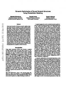
For example, let X 1 , X 2 , X 3 denote severity of acute illness, chronic health status, and mortality of a patient, respectively, where chronic health status of the patient was evaluated before the illness occurred, and influences the severity of acute illness. Suppose that both variables X 1 and X 2 influence the chance of mortality
( X3 )
of the patient, see
Figure 2.1.
Severity of acute illness: X 1
X 3 : Mortality
Chronic health status: X 2 Figure 2.1: A Bayesian Network with Three Random Variables of a Patient
Each arc is an ordered 2-tuple Auv = ( X u , X v ) , such that u ≠ v . X u ∈ Pa ( X v ) is said to be a parent of X v , and X v ∈ Ch ( X u ) is said to be a child of X u . A traverse or traversal T is an alternating sequence of nodes and arcs, such that every arc Auv is preceded by a node X u and followed by a node X v . The Bayesian network in Figure 2.1 yields the following four complete traversals: T1 = ( X 1 , A13 , X 3 ) T2 = ( X 2 , A21 , X 1 , A13 , X 3 ) T3 = ( X 2 , A23 , X 3 ) T4 = ( X 3 )
30
(1.7)
A shorthand notation for traversal and paths excludes the arcs, since there is a unique arc between two adjacent nodes.19 From this point on, this shorthand notation is always used in this dissertation. Notice that if the arc A23 in Figure 2.1 is replaced with an arc A32 , S would exhibit a cycle and T2 in the traversals set (1.7) would be an infinite sequence. In S every possible T is a path, and thus finite. In a path, every node (therefore every arc)
is distinct. In other words, S does not contain a cycle; therefore, S is said to be a directed acyclic graph. In this dissertation, the concept of path is used to validate every arc that may be added into a Bayesian network and might cause a cycle. Parameters are the terms that define the distribution of the model, which represents the population distribution Φ (Bernardo & Smith, 2000). For example, suppose body weight X in a population is distributed normally, i.e. Φ ( X ) ∼ N ( µ ,σ 2 ) , where µ and σ are the mean and standard deviation of this population distribution, which can be estimated from the sample and compose together the parameter set of the body weight model. In this dissertation, only multinomial Bayesian networks are discussed; therefore, the nature of the parameters of interest is multinomial. Suppose we have a sample of size N from a sample space of size k, i.e. Ω = (ω1 ,…, ωk ) , where probability of each distinct outcome is denoted by θi = P ( X (ωi ) ) . Let each frequency count of X (ωi ) in the sam-
19
Since Bayesian network structures are not hypergraphs, which are not considered here. For details, see (Harary, 1969).
31
ple of size N be denoted by ni = n ( X (ωi ) N ) .
The size of the event space20 is com-
puted through the multinomial coefficient, n 1
N n2
N! . = ' nk n1 ! n2 !' nk !
(1.8)
The joint probability distribution of this multinomial sample can be obtained as follows: P ( X (ω1 ) = n1 ,…, X (ωk ) = nk ) = n1
N n2
n1 n θ1 'θ k k ' nk
(1.9)
As seen in Equation (1.9), the parameters that define the multinomial distribution are the sample size N and the probabilities, θ1 ,…,θ k . While the parameters define the state of the domain, the parameter space Θ is the space of all states of the domain, where θ ∈ Θ (Berger, 1985). In mathematics, the dimension of a model usually refers to the number of variables of model; e.g., a Bayesian network M with n random variables is an n-dimensional model, which is denoted in this dissertation by dim X ( M) . In this dissertation, the number of parameters required to model a random variable is called the parametric dimension and it is denoted by dimθ ( M) as is discussed below. As seen in Equation (1.9), the number of different joint distributions increases as a function of both N and k. The larger the parameter space, the more complex the functions that we can represent. If we consider the same issue from the reverse perspective, when the
20
The number of distinct possible events, or the number of different arrangements of the sample among k distinct outcomes.
32
parameter space increases, the number of distributions that might generate the data increases as well. Identifying the distribution that best fits the data based (based on a metric) may require extensive search, which comes with high computational time complexity. This phenomenon is known as the curse of dimensionality or the dimensionality problem. While nodes, arcs, and parameters are basic building blocks of a Bayesian network, another functional decomposition of a Bayesian network is often needed: A Bayesian network is a composition of a set of local structures and local parameters. Let local structure Li be associated with a variable X i such that: ∀i : Li = { X i , Pa ( X i )}
(1.10)
Pa ( X i ) = {Pa1 ( X i ) , Pa2 ( X i ) ,…, Paπ ( X i )} ,
(1.11)
where Pau ( X i ) denotes a particular parent variable of X i and Pa ( X i ) denotes all parents of X i . The set of all local structures S = {L1 , L2 ,…, Ln } is referred to as the global structure. Correspondingly, the global set of probabilities θ consists of local probabilities, that is
θ1 ,θ 2 ,…,θ n , where ∀i , ∀j ≠ i : θi ∩ θ j = ∅ . Outcomes of every variable considered in this dissertation are finite, hence countable, and are enumerated by # + , such that X i = {1,2,…, ri }
33
(1.12)
Probabilities of a random variable are
θ1 ,θ 2 ,…,θ r ,
(1.13)
P ( X i ) = {P ( X i = 1) , P ( X i = 2 ) ,…, P ( X i = ri )}
(1.14)
i
which correspond to
The parametric dimension of a multinomial random variable denoted by dimθ ( X i ) is
{
}
dimθ ( X i ) = θ1 ,…,θ ri −1 ,
(1.15)
which is also called the minimal sufficient statistics or in short the sufficient statistics21 for X i . A set of sufficient statistics is the summary of “the whole of the relevant information supplied by the sample” (Fisher, 1922). A statistic (e.g., σ , n ( X i N ) , or θ1 ) is a function of the sample. Notice that one of the θi terms in Equation (1.13) is absent in Equation (1.15), because given sufficient statistics and the last axiom of probability theory, the remaining probability can be deduced by subtracting the sum of probabilities from 1. In other words, sufficient statistics entail all parameters that are necessary and sufficient to obtain the joint probability distribution as shown in Equation (1.9). The sample space of Pa ( X i ) is the set of combinations of outcomes of Pa ( X i ) , where each distinct combination of outcomes of Pa ( X i ) is called a parent configuration of X i denoted by Ci = {Cij } . ∀j
21
The term sufficient statistics sometimes is used in singular form, sufficient statistic, even if it corresponds to two or more parameters.
34
{
Ω ( Pa ( X i ) ) = Ci1 , Ci 2 ,…, Ciqi
}
(1.16)
Suppose in our example, the variable chronic health status is evaluated as low, normal, high, which can be enumerated as X 2 = {1,2,3} , respectively, and let the other two variables be binary. The parent configurations of X 1 are as follows: C11 = { pa1 ( X 1 ) = 1} = { X 2 = 1}
C12 = { pa2 ( X 1 ) = 2}= { X 2 = 2} C13 = { pa3 ( X 1 ) = 3} = { X 2 = 3}
The parent configuration of X 2 is as follows: C21 = {
}
Notice the last subscript of a configuration set Ci is qi (see Equation (1.16)), and the last and only term for C2 is C21 , i.e., q2 is 1, i.e. q2 ≠ 0 . The parent configurations of X 3 are as follows: C31 = { X 1 = 1, X 2 = 1} C32 = { X 1 = 1, X 2 = 2} C33 = { X 1 = 1, X 2 = 3} C34 = { X 1 = 2, X 2 = 1} C35 = { X 1 = 2, X 2 = 2} C36 = { X 1 = 2, X 2 = 3} Similarly, the sample space of Li is the set of combinations of outcomes of Li , where each distinct combination of outcomes of Li is called a node-parent configuration of X i or a local structure configuration of X i denoted by Cijk is defined similarly:
35
Cijk = { X i = k , Cij }
(1.17)
Ω ( Li ) = {Cijk }
(1.18)
qi , ri j =1, k =1
The local structure configurations of X 1 is as follows: C111 = { X 1 = 1, C11 } = { X 1 = 1, X 2 = 1} = (1,1)
C112 = { X 1 = 2, C11 } = { X 1 = 2, X 2 = 1} = ( 2,1)
C121 = { X 1 = 1, C12 } = { X 1 = 1, X 2 = 2} = (1,2 ) C122 = { X 1 = 2, C12 } = { X 1 = 2, X 2 = 2} = ( 2,2) C131 = { X 1 = 1, C13 } = { X 1 = 1, X 2 = 3} = (1,3)
C132 = { X 1 = 2, C13 } = { X 1 = 2, X 2 = 3} = ( 2,3)
The parametric dimension of a local structure is
{
}
dimθ ( Li ) = θ ( Li ) = N ;θi11 ,…,θi1ri ,θi 21 ,…,θiq ( r −1) = ri qi i
i
(1.19)
In our example, dimθ ( L1 ) , dimθ ( L2 ) , dimθ ( L3 ) are 2 ⋅ 3 = 6 , 3 ⋅ 1 = 3 , and 2 ⋅ 6 = 12 , respectively. In our example, every node is connected to every other node. Such a structure is called a clique and denoted by K n , where n is the dimension of K, i.e. the number of nodes in the clique. The parametric dimension of a clique depends on the size of the set of the joint probabilities of its variables, and it is computed as follows: n
dimθ ( K n ) = ∏ ri
(1.20)
i
Again, the parametric dimension of a clique consists of sample size N and all joint probabilities except arbitrarily one of them. For a given variable set of size n , K n delineates
36
the upper-bound time and space complexity of n-dimensional model; therefore, dimθ ( K n ) plays an important role in complexity analysis.
2.4.2 Learning Bayesian Network Structures from Complete Data Finding one Bayesian network that fits the data better than another Bayesian network requires a search over the model space. Each step of the search involves using a metric in the evaluation of the model. Searching for the most likely network is called model selection. The success of model selection depends on the efficiency and effectiveness of the search heuristic22 and the scoring metric. Although there are many model scoring metrics, such as information theoretic metrics (e.g., the Akaike Information Criterion (AIC), Bayesian Information Criterion (BIC), and Kullback-Leibler divergence) and conventional goodness-of-fit metrics (such as chisquare statistic, Pearson’s chi-square statistic, and likelihood ratio statistic), the focus in this study is on BDe, a Bayesian model scoring metric used to score Bayesian networks. The most distinguishing property of Bayesian scoring metrics is the combination of data with subjective prior probabilities on model parameters and model structures, which are called “parameter priors” and “structure priors,” respectively. A Bayesian network with n variables { X 1 ,..., X n } can be scored using the BDe metric (Cooper & Herskovits, 1992; Heckerman et al., 1995), which is as follows:
22
In real-world problems, the model space is usually too large to search exhaustively; thus, a heuristic search needs to be adopted.
37
n
qi
i
j
P ( S | D ) ∝ P ( S ) ∏∏
Γ (αij )
Γ (αij + N ij
ri
)∏ k
Γ (αijk + N ijk ) Γ (αijk )
.
(2.21)
The score P ( S | D ) indicates the probability of a Bayesian network structure S for a given sample (i.e., data) D. It is also called a posterior probability, or simply posterior. P ( S ) is a structure prior determined by the network developer. The terms ri and qi de-
note the size of sample space of X i and that of Pa ( X i ) , respectively.
Let
Cijk = ( X i = k , Pa ( X i ) ) denote a configuration of a local structure and α 0 denote the prior equivalent sample size, which corresponds to the size of an (imaginary) prior sample that shaped our belief on the population distribution Φ , then N ijk = n ( Cijk N ) and
αijk = ( Cijk α 0 ) are the frequency count and prior parameter of Cijk , respectively, and N ij = ∑ kri N ijk and αij = ∑ kri αijk . As seen in Equation (2.21), the score of each local structure { X i , Pa ( X i )} is computed independently, and each local score contributes to the global score as an independent multiplicative factor. The BDe metric makes the following assumptions (Heckerman et al., 1995): 1. Multinomial Sample: The sample contains categorical data only. 2. Complete Data: There are no missing data in the sample.
38
3. Parameter Modularity: Let θ ijk denote P ( X i = k | Pai = j ) . Given N, parameters of Cijk are modular: If X i has the same set of parents in two different Bayesian networks with structures S1 and S 2 , for which P ( S1 ) > 0 and P ( S 2 ) > 0 , then
∀j f (θij | S1 ) = f (θij | S2 ) , where θij = {θij1 ,...,θijn } .
(
)
4. Dirichlet Parameter Distribution:23 θ ∼ Dirichlet α111 ,...,α ijk ,...,α nqn rn .
The
Dirichlet parameter distribution assumption implies that given S, there exists a set of parameter priors {αijk } so that Equation (2.22) holds:
f (θij | S ) =
( ) θ ∏ Γ (α ) ' Γ (α )
Γ αij1 + ' + αijri ij1
ijri
ri
k =1
α k −1
(2.22)
ijk
Equation (2.22) implies that given parameter priors, elements of θij are a priori independent. 5. Parameter Independence: The parameters of the population are independent. This assumption is divided into two parts, Local and Global Parameter Independence. a. Local Parameter Independence: The elements of θij are independent. This assumption allows the expression of priors associated with variable Xi as
{
}
follows: ∀i f (θ i | S ) = ∏ ji=1 f (θ ij | S ) , where θ i = θ i1 ,...,θ iqi . q
23
If all the probability density functions are assumed to be strictly positive, i.e. ∀ ( i, j, k ) θijk > 0 , the
condition of this assumption is shown to be a necessary consequence of assumptions 5.a and 5.b (Geiger & Heckerman, 1995).
39
b. Global Parameter Independence: The parameters of different variables are independent. This assumption facilitates the computation of the parameters θ of a Bayesian network B = ( S ,θ ) as a product of the parameters of individual variables: ∀i f (θ | S ) = ∏ i =1 f (θ i | S ) , where θ = {θ1 ,...,θ n } . n
6. Prior equivalent sample: Prior belief about parameters defined on S can be conceptualized as if a number of cases (a sample of size α 0 ) had already been observed and ∀ ( i, j, k ) : αijk = α 0 P ( X i = k , Pa ( X i ) = j ) . The term α 0 is called the
prior equivalent sample size. The hypothetical Bayesian network with the structure S and parameters {αijk }∀ i , j ,k is called a prior Bayesian network. (
)
The BDe metric without Assumption 6 is called the BD metric. With the addition of prior equivalent sample assumption, it exhibits the likelihood equivalence property (Heckerman et al., 1995); which means that if two Bayesian network structures S1 and S 2 are statistically indistinguishable then P ( D | S1 ) = P ( D | S 2 ) . The term P ( D | S ) is
called the marginal likelihood. Two Bayesian network structures are statistically indistinguishable if they (1) have the same set of conditional independence relations according to the Markov condition, (2) have prior probabilities derived from the same prior network, and (3) use a constant prior equivalent sample size α 0 where ∀i : α 0 = α i = ∑ j ,k α ijk , (Spiegelhalter et al., 1993). The BDeu metric is a special case of the BDe metric in which ∀ijk : α ijk =
1 . qi ri
40
2.4.3 Parameterization and Inference in Bayesian Networks
In this dissertation, the probability terms {θijk } are computed as follows:
θijk = P ( X i = k Pa ( X i ) = j ) =
N ijk + 1 N ij + ri
(2.23)
This approach of parameterization, which is called smoothing differs from maximum likelihood estimation, in which θijk = N ijk N ij . Notice that if N ij = 0 (hence, N ijk = 0) , the
probability term in Equation (2.23) remains strictly positive and equals 1 ri . This latter term, which is called a Bayes-Laplace prior (Jaynes, 1968) indicates that our prior belief about θijk values are uniform for every k . The Bayes-Laplace prior can be applied differently than as it is used in Equation (2.23) by putting more (α > 1) or less (α < 1) weight on the priors:
θijk =
N ijk + α
(2.24)
N ij + α ri
Prior belief certainly does not have to be uniform; therefore, the general form of Equation (2.23) is
θijk =
N ijk + α ijk N ij + α ij
,
(2.25)
where α ij = ∑ ki αijk . r
Recall that a Bayesian network can be decomposed into a set of local structures. The joint probability distribution of a Bayesian network is computed as a product of prob-
41
abilities of child variables given their parents. This method is also known as recursive factorization. n
P (θ ) = ∏ θijk i =1 n
(
= ∏ P X i Pa ( X i ) i =1
)
(2.26)
= P ( X 1 ,…, X n )
The variables of the Bayesian network in Figure 2.1 can be sorted based on their topological order:
( X 2 , X1, X 3 ) .
A set is ordered topologically if the following condition
holds for every variable for every position i = 1,2,… : Every parent of the variable in position i is in a position that is less than i. The recursive factorization of the Bayesian network in Figure 2.1 is: P ( X1, X 2 , X 3 ) = P ( X 2 ) P ( X1 X 2 ) P ( X 3 X1, X 2 )
(2.27)
In moderately large Bayesian networks such products can be efficiently computed using the local computation or junction tree algorithm (Lauritzen & Spiegelhalter, 1988), which is the main inferential method used in the experiments of this dissertation (for further details, see Section 2.4.6). The junction tree algorithm is an exact Bayesian network inference method. Exact Bayesian network inference is to be NP-hard (Cooper, 1990). In those cases when exact inference is not practical, other approximate algorithms are used, for which I used likelihood weighting algorithm. For details of this and other well known approximation algorithms, see (Cousins, Chen, & Frisse, 1993; Shachter & Peot, 1990).
42
2.4.4 Dynamic Bayesian Networks
A dynamic Bayesian network (DBN) is a Bayesian network with explicitly represented temporal variables. A DBN structure can be viewed as having two dimensions: The time line and the variable line represented on the horizontal and vertical axes, respectively see
Figure 2.2. TEF X ( t0 )
X ( t1 )
X ( t2 )
X ( t3 )
X1 ( t ) X2 (t) X3 ( t )
past
present
future
time
Figure 2.2: A DBN with Four Time Slices Each variable on the time line forms a sequence X i ( t ) = { X i ( t0 ) ,…, X i ( td )} called a temporal variable sequence (TVS); the sequence of TVS values for a given patient is
called the temporal outcome sequence (TOS). At a given time (time slice) tk , there exists
{
a set of variables X ( tk ) = X 1 ( tk ) = x1( k ) , …, X n ( tk ) = xn( k )
}
called a contemporaneous
variables set (CVS). Temporal variables are measured at the same time are said to be contemporaneous. Outcomes of a CVS (i.e., x1( k ) ,…, xn( k ) ) forms a contemporaneous outcomes set (COS). As discussed in Section 2.3, in this dissertation time index set T = ! ,
43
which is equivalent to interval-valued time parameter on the real line; therefore, in this dissertation, the terms time point and time slice are used interchangeably. As discussed in Background section about Markov processes, a TVS can be an infinite sequence. When the context reveals a fixed initial time t0 and a known terminal time td , (e.g., admission and discharge of a patient who stayed in the ICU for d + 1 days), then
(
)
X i ( t ) implies { X i ( t0 ) , X i ( t1 ) ,…, X i ( td )} , which also can be expressed as X i t[0,d ] .
In Figure 2.2, a vertical line called temporal event frontier (TEF) is drawn, which is an imaginary (virtual)24 line of the present time and sweeps from left to right in the direction of time flow. It always is at a certain point on the time line, indicating what time it is relative to the DBN structure. In the example shown in Figure 2.2, all variables that are behind the TEF line have been measured. Variables whose outcomes are known (i.e., measured) are represented as shaded nodes on the graph. In the context of inference, their outcomes (as well as the corresponding nodes) are called evidence. DBNs can be decomposed into a set of local structures as Bayesian networks are decomposed. Additionally, they can be decomposed into a set of time slices, or into a set of local structures over a sequence of time slices. Each such decomposition yields a different type of subprocess since a DBN as a whole represents a (global) stochastic process. The smallest building block of a stochastic process may be called an elementary subprocess, which is represented in DBNs as a temporal local structure Li ( t ) .
24
In other words, TEF is not an actual data structure as nodes, arcs, and parameters are, but it can be conceptualized as a control structure (like a flag) indicating relative time and the current state of collected information.
44
Temporal problems bring useful background knowledge that may be incorporated within the structure of DBNs. The foremost important information is that variables are temporally ordered and that the direction of dependencies between variables is the same as the direction of time. As seen in Figure 2.2, there is no arc that is extended from right to left (against the time flow). Being in a compliance with the direction of time, variable interactions could be perceived as causal interactions, which may or may not be true (Glymour & Cooper, 1999; Spirtes, Glymour, & Scheines, 2000; Pearl, 2000). In this dissertation, all variable interactions are associational, with no commitment as to whether they are causal. Since we use the DBN models for predictions that are based on observations, rather than on interventions, distinguishing causal relationships (arcs) from associational ones is not necessary. The current trend in DBN research is to find efficient methods to parameterize manually constructed DBN structures, which sometimes were built explicitly with some causal interpretation, see e.g. (Dagum et al., 1995; Kjaerulff, 1992; Arroyo-Figueroa, Alvarez, & Sucar, 2000; Tawfik & Neufeld, 2000). Therefore, in literature DBNs25 have about the same conformation as the one shown in Figure 2.2. More subtle but important background knowledge that can be incorporated readily into search over the space of DBN structures is the expectation of a dependency between successive instances of a TVS, i.e., { X i ( t ) , X i ( t + 1)}∀t ; e.g., serum-glucose level at time t depends the serum-glucose level at time t − 1 . If the data-sampling rate is high, as in sig25
Although every Bayesian network that has a nonempty set of variables with an explicit time dimension and/or a set of space dimension (as in biological sequence analysis) can be classified as a DBN, such labels are not common in literature.
45
nal processing, it may be reasonable to assume that there are no dependencies between contemporaneous variables; i.e., variables in the same time slice would be assumed independent given the outcomes of earlier events. There are other rules that are usually found to be effective in heuristic search for DBN models. For example, information in the recent past is likely to be more important for predicting future outcomes than the information in the distant past. Such heuristics can significantly constrain the search space, making search of complex temporal models more feasible computationally. Markov processes, defined by Equation (2.2) can be represented in DBNs, such as the one shown in Figure 2.3, where the restriction is that arcs can span between at most two time slices. X ( t0 )
X ( t1 )
X ( t2 )
X ( t3 )
X1 ( t ) X2 (t) X3 ( t )
time
Figure 2.3: A Markov Process as a First-Order DBN The DBN in Figure 2.3 is not stationary. In the example DBN shown in Figure 2.3, the local structure of
X 3 ( t2 ) , (i.e.,
{X
3
( t2 ) , Pa ( X 3 ( t2 ) )} ,
46
where its parents are
Pa ( X 3 ( t2 ) ) = { X 3 ( t1 ) , X 2 ( t2 )} ) is different than other instances of the local structures of X 3 ( t ) . By the definition of stationarity, joint probability distributions of these local
structures have to be equivalent; thus, a systematic structure learning process has to yield isomorphic26 local structures (i.e., symmetry between every pair of local structures) for the entire DBN. The only exceptions are the local structures of the initial condition X ( t0 ) , if there is any. Although structural stationarity (i.e., the repeating symmetry of
arcs within each CVS and between every pair of adjacent CVSs) is not a sufficient condition for stationarity, it is certainly a necessary condition. Compliance with stationarity can easily be achieved for the DBN structure in Figure 2.3
( )
by deleting the arc in X 3 t[1,2] , or by adding directed arcs in the direction of time flow
(
)
into X 3 t[0,1],[2,3] , whichever yields better score. The resulting structure may compactly be represented in two time slices, such as the structure shown in Figure 2.4.
X (t )
X ( t + 1)
X1 ( t ) X2 (t) X3 ( t )
time
Figure 2.4: Stationary Markov Process as a First-Order DBN 26
Two structures are isomorphic if there is one-to-one correspondence between their sets of arcs and between their sets of nodes.
47
The parameters defined on local structures of the first time slice represent the initial distribution and the parameters defined on the other remaining interactions between variables in the structure represent transition probabilities (see Section 2.3). 2.4.5 Learning Structures of DBNs from Complete Data
Although the earliest accounts of DBNs in literature date to the late 1980s (Cooper et al., 1988; Dean & Kanazawa, 1989), DBNs have been used increasingly in the second half of the 1990s. DBNs have been applied successfully to a number of problems, including ICU patient outcome predictions (Dagum et al., 1995), liver transplantation process models (Aliferis & Cooper, 1998), diabetic patient monitoring (Bellazzi et al., 1998; Bleckert et al., 1998; Hovorka et al., 1999), speech recognition (Zweig, 1998; Bilmes, 2000; Stephenson et al., 2000), user modeling (Schafer & Weyrath, 1997), power plant process modeling (Arroyo-Figueroa et al., 2000), map learning for mobile robots (Doucet et al., 2000), and motion analysis and control (Forbes et al., 1995). Aliferis and Cooper recently extended the conventional DBN representation with constructs that represent levels of temporal abstractions. They called the resulting representation Modifiable Temporal Bayesian Networks (MTBNs) (Aliferis & Cooper, 1995; Aliferis, 1998). The MTBN approach introduces a different temporal indexing method for temporal variables, which enables one to specify different temporal granularities and different levels of temporal abstractions for every subset of variables. The levels of temporal abstractions represented in an MTBN enables model developers to work on more compact graphs, while its new notation captures some temporal specifications that augment the set of temporal indices found in conventional DBNs. The dissertation hypothe48
ses do not require additional features that MTBN representation offers; therefore, its representation was not used in this dissertation. Dagum et al. (Dagum et al., 1995) were one of the first investigators on dynamic Bayesian networks and applied their work on ICU domain, where they monitored central hemodynamics of an ICU patient. Measurements of mean arterial blood pressure, heart rate, arterial and venous oxygen saturations, oxygen consumption and carbon dioxide production were taken and monitored with an 11-minute periodicity. They constructed a causal DBN structure, where we can distinguish two sets of nodes: (Set 1) all four variables to be predicted were placed in front of the TEF, whereas (Set 2) all other variables were behind TEF (i.e., their measurements were known); thus, variables in Set 2 were directly connected to variables in Set 1. Although not learned from data, the structure had an interesting long-term temporal dependency property as shown in Figure 2.5 (incoming arcs into VO2 ( t0 ) from other variables are not shown). This structure combines information of near-term (11 and 22 minutes) outcomes with a single long-term (approx. 12 hours) outcome. X ( t−2 )
X ( t−69 )
X ( t −1 )
X ( t0 )
VO2 ( t )
time
Figure 2.5: Monitoring VO2 on an ICU Patient (Dagum et al., 1995)
49
Learning DBN structures from data is a relatively new research direction. To my knowledge, the first investigation of DBN structure learning was reported study in (Friedman, Murphy, & Russell, 1998) who modeled human car driving conditions in a simulated environment. The data contained tracking information with the following variables: position and speed relative to a roadside reference, distance and speed relative to the car in front, (Boolean) presence of a car immediately to the left or right. Three models were learned with 0, 1, or 2 hidden variables. Learning was performed using two different scoring metrics (BDe and BIC) under the stationary Markov process assumption and was decomposed into two tasks: 1) Learning X ( t0 ) , and 2) learning a transition network. The structure of a transition network comprises all nodes in a CVS such that X ( t ≠ t0 ) and all incoming arcs to the nodes in that CVS. In the presence of hidden variables, they combined existing metrics (either BDe or BIC) with a version of EM algorithm to learn DBN structures. The authors argued that the set of arcs within time slice t0 does not need to be equivalent (i.e., bijective) to the set of interactions within any other time slice t > t0 . While a different set of interactions within X ( t0 ) does indeed not alter the isomorphic nature (imposed by stationarity) of the local structures in other time slices, the benefits (if any) of learning interactions within X ( t0 ) separately are not clear.27
Some other authors
(Davies, 2002; Murphy, 2002) followed this decomposition scheme in estimating DBN parameters. In the context of learning models from complete data for prediction, in this
27
For further details about the rationale, see (Friedman et al., 1998).
50
dissertation we do not need to learn the interactions within X ( t0 ) , since the presence of evidence at t0 is given, and thus any interactions between the variable at t0 nodes will not have an effect on predicting mortality beyond t0 . In the absence of evidence, the DBN structure
is
immaterial
for
inference
purposes,
because
for
any
variable
P ( X i ( td ) = k E = ∅ ) can be directly estimated from statistic (see Section 2.4.3). P ( X i ( td ) = k E = ∅ ) =
1 + ∑ t N i1k ( t ) ri + ∑ t N ( t )
(2.28)
Learning in (Friedman et al., 1998) was performed on various size datasets. Dataset sizes were different for learning tasks 1 and 2 (see above). They varied between 250 and 1500 for the learning task 1, and between 104 and 105 for the learning task 2. Interactions within X ( t0 ) were learned without assuming stationarity by using frequency counts of only those outcomes that occurred at time t0 , whereas learning interactions in other time slices were performed under stationarity assumptions. Another study on learning dynamic structures (Bilmes, 2000) was performed on a class of hidden Markov models (HMMs). The model class that Bilmes focused on is called autoregressive HMM, or AR-HMM(K), see Figure 2.6.
51
X ( t0 )
X ( t1 )
X ( t2 )
X ( t3 )
X1 ( t ) X2 (t)
time Figure 2.6: Auto-Regressive Hidden Markov Model with Second-Order Markov Dependencies In an HMM, unobserved state variables (seen as unshaded nodes in Figure 2.6) yield observed outputs, which are independent conditioned on the state variables. In AR-HMMs, outputs are also first-order Markov dependent; whereas, in AR-HMM(K) model, Kthorder dependencies are allowed. In his study, using an information theoretic (mutual information) metric, Bilmes scored contributions of higher order arcs conditioned on variable values; thus, the presence of a higher-order dependency was influenced by a given state of variables. A Bayesian network associated with two or more structures that vary among different observations is called a multinet (Geiger & Heckerman, 1996). In one of our earlier studies (Kayaalp et al., 2000, see APPENDIX A) , we learned DBN structures from a SOFA dataset (Vincent et al., 1996) using the K2 Bayesian network scoring metric (Cooper & Herskovits, 1992). Using forward-stepwise arc-addition algorithm, we searched arcs, which were in the direction of time flow. The survival outcome was in the last time slice td . Search for the predictors of the outcome was performed over time slices {t < td } . The resulting Bayesian network had a simple structure with a
52
single predictor of survival, which was total SOFA score. The stationary model outperformed the average of all (33) nonstationary models.
Each nonstationary model
i = 1,…,33 was parameterized by the data of patients who stay in the ICU exactly i days. No independencies were assumed. Nonstationary models of patients who stayed in the ICU very short periods consisted of larger sample sizes than other nonstationary models and performed relatively better than other nonstationary models in terms of predictive performance. The results were interpreted as the performance of a nonstationary model may be comparable to that of a stationary model, if there are sufficient data to parameterize the nonstationary model. That study was the precursor of the experiments of this dissertation. In a later study (Kayaalp et al., 2001, see APPENDIX B), we studied an alternative approach to learn DBN structures from data. In this study, new variables were constructed by sequences of outcomes observed in the sample. Then those variables were rank ordered based on how well they predicted survival according to a receiver operating characteristic (ROC) metric (see Chapter 4.4). A set of m variables that were listed on top of the rank were input into a simple Bayes network and survival chances was predicted in the near and relatively distant future times. The size m was determined by cross-validation. By combining data sequences of varying lengths, we effectively combined different order Markov models and different stationarity assumptions. Other research on DBNs involves a focus on parameter estimation including the use of EM (Lauritzen, 1995), gradient-descent (Russell et al., 1995; Binder et al., 1997), various smoothing and filtering algorithms with linear Gaussian distributions (such as Kalman filters, linear update filters), with mixture of Gaussian distributions (such as assumed 53
density filters, and Gaussian sum filters)28 and various other sampling and approximation algorithms such as MCMC (Shachter & Peot, 1990; Chickering & Heckerman, 1996). This line of research is outside of the focus of this dissertation, and extensive reviews can be found elsewhere (Forsythe, 1992; Murphy, 2002; Murphy, To Appear) Markov decision processes (MDPs) are another temporal probabilistic network representation and are frequently used in planning and robotics. MDPs are defined on state spaces (see the discussion on state spaces of Markov processes in Section 2.3). A detailed treatment of differences and similarities between DBNs and MDPs can be found in (Boutilier, 1999).
2.4.6 Inference in Dynamic Bayesian Networks Although the methodologies proposed, tested, and evaluated in this dissertation are not about inference, their evaluation requires the use of inference. In DBNs as mentioned in Section 2.4.3, there are two major classes of inferential techniques: exact inference and approximate inference. Exact inference is preferable, when computationally feasible; however, exact methods may require more computational resources than are available. In that case, a suitable approximation method can be used. Exact inference on Bayesian networks is usually performed through the local computation algorithm (Lauritzen & Spiegelhalter, 1988), which also is the main inference method used in testing the models of this dissertation. Local computation (a.k.a. junction tree) algorithm converts each local structure separately into a clique, and the Bayesian 28
For an extended set of research areas on filtering and smoothing, see T, Minka’s overview on Bayesian Inference in Dynamic Models: http://www.stat.cmu.edu/ ~minka/dynamic.html
54
network into a chordal graph G1 , which then is transformed into a junction tree G2 such that each maximum clique K a of G1 is mapped onto a node va of G2 , and every node pair ( va , vb ) of G2 is connected through an undirected edge if K a ∩ K b ≠ ∅ . The joint probability of this graph can be computed as
P (X) =
∏ P(K ) ∏
K∈G1
( va ,vb )∈G2
P ( K a ∩ Kb )
.
(2.29)
In Equation (2.29) P ( K ) ≡ P ( X ′) , in which P ( X ′) is the joint probability of variables, and X′ and {v ∈ K }∀v are bijective (i.e., they are in one-to-one correspondence), where
{v} denotes the vertex set of K. The local computation algorithm is perhaps the most popular exact method that is used for Bayesian network inference. Other alternative exact methods such as the arc reversal algorithm (Shachter, 1986) can also be found in the literature. For an extended summary of the local computation algorithm and descriptions of other frequently used inference algorithms, see (Pearl, 1988; Lauritzen, 1996; Dechter, 1998; Cowell, 1998b). Although approximate inference is of great interest in DBN research, it is not directly related to the hypotheses of this dissertation, and, in fact, a reasonable treatment of this very wide area of research is outside the scope of this dissertation. There are a number of overview articles, such as (Murphy, To Appear; Shachter & Peot, 1990; Cousins et al., 1993; Jordan, Ghahramani, Jaakkola, & Saul, 1998; Cowell, 1998a), dissertations such as
55
(Kozlov, 1998; Davies, 2002; Murphy, 2002) and other relevant publications such as (Boyen & Koller, 1998; Nodelman, Shelton, & Koller, 2002).
2.4.7 Instance-based Learning It is more important to know what kind of a patient has a disease than what kind of a disease a patient has. — Sir William Osler, M.D., 1891 Medical wisdom dictates that the clinical approach ought to be patient centric rather than disease centric. The instance-based learning approach described below enables us to build patient-specific models that respect this medical wisdom. It is important to note that the patient-specific (or, in more general terms, case-specific) model learning approach proposed, implemented, and tested in this study is based on the instance-based approach, but it is different from mainstream instance-based learning methods. These differences are discussed in Section 3.3. In conventional supervised-learning techniques, a classification model is built using the known cases provided in a training set. Subsequently, this single model is used to classify all test (query) cases selected from the same population as the training cases. This process is illustrated in Figure 2.7, where Query (i) represents the ith case to be classified. While the first module, Model Building, takes place only once, the Classification module must be executed n times if there are n query cases to be classified. The model is usually optimized for predicting the majority of the cases prevalent in the training set ; otherwise, in the long run, the overfitting problem would be likely to lower the predictive performance of the model (Mitchell, 1997). Therefore, the types of cases that are underrepresented in the training set are usually classified with low accuracy. 56
Classification (i)
Model Building
Sample
Model
Query (i)
Model
Classification
Figure 2.7: Model building and classification in conventional supervised-learning techniques. On the other hand, in the instance-based learning approach, the model building takes place after a query case is provided to the learner. As shown in Figure 2.8, a different model is built for each query case; therefore, the entire learning process must run n times if there are n unknown cases to be classified. With instance-based learning, unusual cases are modeled with relatively high fidelity, subject of course to intrinsic limitations of the training set.
Model Construction and Classification (i) Sample Query (i)
Model (i)
Classification (i)
Figure 2.8: Model building and classification in the instance-based learning approach
The differences between these two approaches are not only mechanistic but also conceptual: In conventional modeling approaches, it is not feasible to learn a general model without knowing the types of query cases a priori. Conventionally, a model is built with a specific question in mind, e.g. whether a case is or is not a member of a class. Such restrictions do not exist with instance-based learning approaches. For example, if the entire database of a fully automated healthcare system is used an instance-based learning system can dynamically construct a model to classify a patient case for diagnostic, therapeu57
tic, prognostic, or any other purpose as long as the information in the database is adequate for the required inference and there are sufficient patient data to make such inferences. In a statistical instance-based learning approach, the problem is to identify the set of training cases that are “similar” to the query case and to classify the query case using the statistic that is obtained from the training set of these similar cases. The measure of similarity between the query case and the training cases is based on the attributes of the query case that are represented in the model. In the nearest-neighbor method, the similarity between the query case and the training cases is determined by some given metric, which often is a Euclidian distance metric due to its simplicity and intuitiveness. However, other metrics such as the Minkowski metric, the Manhattan distance, and the Tanimoto metric can be used as well (Duda, Hart, & Stork, 2000). The set of variables (attributes) that best discriminate the outcome of a query case is expected to be much smaller in the instance-based learning approach, because a population model ought to provide solutions to the union of all probable query cases. The population-model needs to include the set of variables that might be predictive for any query case, or at least for any very likely query case; thus, the search space of variables can be quite large. As an example, although the set of variables representing routine measurements (age, pulse, blood pressure, etc.) are similar among the ICU patients, the set of measured laboratory tests and medications vary widely among patients. Similarly, the number of days of ICU stay also varies from patient to patient. Thus, in this example, the selection of a population model requires a search over the model space that incorporates the union of medications and lab tests for all the patients in the training set; in contrast, 58
the selection of variables in a patient-specific model requires a search over the space that incorporates only the medications and labs tests of the single patient in question. Let dimθ ( M) denote the parametric model dimension (see Section 2.4.1) of a problem at a given time. An increase in the parametric model dimension is exponential in the order of the process; therefore, the complexity of the search-space of a DBN model M
(
)
with a maximum of t time slices is O dimθ ( M) . t
A generic model ought to provide solutions to a large set of queries that can be formulated as P (Outcome = True | X 1 ,..., X n )
(2.30)
The number of possible queries is the product of the dimensions of every conditioning variable,
∏
n i =1
dimθ ( X i ) ; whereas a model constructed through an instance-based learn-
ing approach is required to provide a solution to a single query that can be formulated as P (Outcome = True | X 1 = x1 ,..., X n = xn ) .
(2.31)
Considering (1) the dimensionality problem aggravated by the inclusion of the temporal dimension, (2) variations in the ICU stay among patients, and (3) the wide spectrum of the clinically relevant variables of patients, patient-specific learning presents an appealing approach relative to learning generic models for a large set of patients. Beside its aforementioned benefits, instance-based learning also allows dynamic discretization instead of off-line a priori discretization, but testing the discretization effectiveness of patient-specific learning is not part of the hypothesis set of the present study; hence, it 59
has not been implemented in this present dissertation study. In related work, Munos and Moore (To appear) showed that instance-based approaches can be used to discretize Markov decision processes to achieve optimal control using various measures. Due to a postponement of the model construction until the presentation of a query case to the learner, the instance-based learning approach is sometimes called lazy-learning (Aha, 1997). Since the cases in the ICU database are patients, the term “patient-specific learning” is more descriptive in the context of this study. Memory-based learning is another term associated with this approach (Stanfill & Waltz, 1986), because all training cases ought to be stored in order to classify new cases; whereas in other approaches, the sample statistic is represented in model parameters, and the training cases are no longer needed for classification. Other terms that have been used in machine learning literature to refer to the instance-based learning approach are case-based reasoning29 and exemplar-based reasoning (Porter, Bareiss, & Holte, 1990). The basic notion among all instance-based methods is that the available training set is not large enough and/or is not distributed homogeneously, as idealized over all training set attributes; thus, the model parameterization cannot be performed reliably over the entire sample space. The premise is that if cases similar to the query case are identified within a subset of the training set, the training set may be replaced by that subset, by which the intended model can be parameterized more accurately. A companion assumption is that the remaining training set that contains all but “similar” training cases cannot be utilized
29
A series of case-based reasoning conferences have been held since 1992. http://www.cbr-web.org/CBR-Web/?info=conferences&menu=rc.
60
For details, see
effectively to extract relevant information for better model parameterization. As discussed in Section 3.3, a patient-specific learning method as implemented in this study does not exclude any single training case in model learning nor does it make the above assumptions. There are a number of parameters that ought to be determined when “similar” cases are identified in the training set, such as •
the size of the subset,
•
the maximum distance between the query case and similar training cases (the terms window size, cell size, or hypercube size are also used),
•
the identification of relevant dimensions (selection of features) of the domain, and
•
the choice of the distance metric that is appropriate for the problem and the data.
The substantial degrees of freedom provided by the above dimensions of instance-based learning make it challenging to compare comprehensively such a learning approach to population-based methods. On the other hand, these degrees of freedom provide ample opportunity for developing instance-based learning approaches that will work well in practice. This dissertation explores once such instance-based learning method, which is described in detail in the next chapter.
61
3
METHODS
This chapter is organized into five sections. In Section 3.1, I describe the ICU data used to test the hypotheses in Section 1.1; which are made more concrete in this section. In Chapter 6, I introduce a new class of DBNs, which I call dynamic simple Bayes models, or in short DSB models. In Section 3.2, I discuss the implementation of the baseline model, which is a DBN representing characteristics of the ICU population. This model is learned from data with the assumption that temporal dependencies are first-order Markovian and the process is stationary. In Section 3.3, I discuss how to learn patient-specific models with the assumption that the underlying process is a stationary Markov process; such models are needed to test the first hypothesis of this dissertation. In Section 3.4, I discuss how to learn patient-specific models without making assumptions on the order or stationarity of the process; such models are needed to test the second hypothesis of this dissertation.
3.1 ICU Data and the Problem The data set used in the present dissertation contains the medical data of 6,704 ICU patients treated in the Presbyterian Hospital of the University of Pittsburgh Medical Center in the 1990’s.30 The database is deidentified; it does not contain names, addresses, social security numbers, or other identifying tags of the patients or the physicians. In this data-
30
I withhold stating the exact time interval in order to protect patient confidentiality in the event this deidentified dataset is made public in the future, with the approval of the Institutional Review Board.
62
set, each patient was assigned a new unique patient number different from his/her medical record number. The dataset includes the records of 6,704 ICU patients: 2,757 females, 3,874 males, and 73 patients whose genders are not indicated. The minimum age is 12 years and the maximum age is 102 years; however, the ages of 64 patients are recorded as “0”, presumably unknown. The data were discretized in consultation with Dr. Gilles Clermont, Assistant Professor in Critical Care Medicine at the University of Pittsburgh and an ICU physician. The variables are listed in APPENDIX C. In this dataset, there are 109 temporal variables and a variable that represents whether the patient survived to be discharged. Not all of these variables were measured every day for every patient. Instead of interpolating their unmeasured values, the value 0 is assigned to those variables, denoting the value as unknown. The meaning of an unknown value is that the value was either some default value (e.g., serum level of a given drug was 0 because the patient was not receiving drug therapy) or the value was not expected to influence the condition or the treatment plan of the patient. It is also possible that some of the data were not entered into the database properly, and therefore, were missing; however, as a simplification method, I assume that there are no such records. Ignoring missing data may certainly add additionally noise into the database but it is not expected to pose a bias in favor of hypotheses of this dissertation. All variables are aggregated into 1-day temporal granularity, which seems a reasonable clinical choice for this domain. It is the temporal granularity adopted in this work for the 63
entire dataset. In earlier studies (Kayaalp et al., 2000; Kayaalp et al., 2001), it was used with satisfactory prediction performance. A more complex choice for this clinical dataset might be a 6-, 8-, or 12-hour temporal granularity, which could be uniform or nonuniform for all variables. A nonuniform temporal granularity scheme may be more suitable when the data collection is automated for the majority of the data or if the data collection frequency for some data is very high (e.g., several times per hour) or continuous (e.g., EKG signal). Certainly, learning the right temporal granularity for each variable would be a more general approach. A heterogeneous temporal granularity scheme, however, is not suitable for this dissertation, because (1) adopting such a scheme would not be appropriate for a baseline model with two time-slices (see Section 3.2), and (2) it would make the scope of the dissertation unmanageable. In this work, if there was more than one entry of a particular measurement for a given patient per day, the median of those measurements was taken. There are other possible choices such as using the mean of the measurements or using the last entry of the day. Certainly, if computational resources are available, an existing variable set can be augmented by introducing new variables that represent parameters of daily distributions (mean, median, variance, minimum, maximum, etc.) of any existing variable. Temporal models learned from data can be used for various clinical purposes, such as monitoring clinical values (in alert systems), diagnosing patient status (in expert systems), forecasting patient outcomes, and determining optimal treatment policies. In this study, the temporal models are learned for forecasting patient outcomes. More specifi64
cally, the models are learned to predict the chance of survival of patients within the subsequent 24 hours of hospitalization. Any clinical variable of patients can be predicted using the same methodology; however, predicting next-day survival has special clinical importance. This problem is also appealing from the view of model evaluation because the outcome to be predicted is very objective. In this study, only a subset of all possible patient variables were used for learning models, since data corresponding to other variables were not readily available. The set of patient variables is much larger due to the multimodal31 nature of the patient data. Examples of the data types that are not used in this study include data related to medications, surgery, and other treatments such as hemodialysis; textual data that are found in patient records such as earlier diagnoses, medical history, op-notes, and progress reports; and imaging and biosignals.
3.2 The Baseline Model This section describes the approach I took to induce baseline models from data. Due to the dimensionality problem (see Section 2.4.1), DBNs are represented in two time slices, and the transition probabilities are assumed stationary over the time span of the problem (Friedman et al., 1998). Such assumptions yield strictly stationary, discrete-time, discrete-state Markov processes. I have adopted the following assumptions to create a
31
Data modality is the nature of the medium on which information is represented. Documents may have heterogeneity in various dimensions, such as physical (e.g., textual, audio, video), organizational (e.g., plots, images), contextual (e.g., discharge report, op-notes, medical history).
65
model whose predictive performance is used as the baseline for evaluating each hypothesis of this dissertation. The Baseline Model assumes: 1. A single model M1 representing relevant clinical processes is learned from the data and used to predict all test cases. 2. The clinical processes represented in M1 are strictly stationary. 3. The clinical processes represented in M1 are Markov processes. Since the hypotheses tested in this dissertation are not about the effectiveness of the model evaluation metric, the same Bayesian metric, BDeu, is used uniformly in all model selection processes. The details of the BDeu metric are provided in Section 2.4.2. In M1 , in addition to atemporal variables, there are two temporal states. In each temporal state, there are n temporal variables (covariates) X = ( X 1 ,… , X n ) and one outcome variable Q . The state of each temporal variable is denoted by a time index t ∈ # such as X i (t ) . The query involves a prediction of the future outcome of a patient given all avail-
able (past and present) data of the patient. The outcome variable has two states: alive and dead (see Figure 3.1). The only non-trivial stochastic problem is the parameterization of the future states of patient outcomes, given the patient is alive at the time point t of the
(
)
query formation. Formally, the query can be stated as P Q ( t + 1) = 1 Q ( t ) = 1, X ( t ) = ? ,
66
where ; i.e., given the patient data at time t, what is the patient’s chance of survival? The term Q ( t + 1) = 1 denotes the outcome state “alive.”
( ) = P (Q ( t + 1) = 1 Q ( t ) = 1) = 1 − p = P (Q ( t + 1) = 0 Q ( t ) = 0 ) = 1 = P (Q ( t + 1) = 1 Q ( t ) = 0 ) = 0
0 < p10 = P Q ( t + 1) = 0 Q ( t ) = 1 < 1 0 < p11 p00 p01
p11
10
P ( D | S1 ) , the newly added arc is not viable. Since ln ( 0 < x ≤ 1) is a monotonically increasing function, the logarithmic transformation appropriately preserves score precedence: ln P ( D | S 2 ) > ln P ( D | S1 ) ⇔ P ( D | S 2 ) > P ( D | S1 ) .
It is important to note that the overall score of a Bayesian network structure is the product of the scores of the local structures, which are the node-parent configurations. Due to the parameter independence assumption of the BDeu metric, each local score is independent of the others; therefore, maximizing every local score maximizes the global score of the structure.
69
The search I use starts by identifying parents of the node representing the outcome variable Q ( td ) , where the time td is the discharge day. Each identified parent of the outcome node may belong to one of two sets: (1) Nodes in time-slice td , and (2) nodes in earlier time-slices {ti }i =1 . Recall that td is the next day. Thus, we are predicting one day d −1
into the future. The values of the outcome variable, Q ( td ) , and indeed all other variables, are thus unknown when the prediction is being made. On the other hand, we assume that all values of all variables on the days before td have known values.32 Because of the Markov property and the no-unknown-values assumption, the only variables that influence the conditional probability distribution of Q ( td ) are those at time td and at time td-1.
(
{
} ,{ X
P Q ( td ) X i ( td ) ∈ Pa (Q ( td ) )
∀i
k
( td −1 ) ∈ Pa (Q ( td ) )}∀k
)
(3.4)
Furthermore, since the values of all the variables at time td-1 have known values, the arcs among these variables have no influence on the conditional probability distribution of Q ( td ) . Therefore, the only variables for which we need to search for parents are those
variables in td that are themselves parents of Q ( td ) . Let U denote this set of variables. The potential parents for the variables in U are the variables in td and td-1. We search separately for the parents of each variable in U, since the scoring metric is decomposable, as mentioned previously. The search for the parents of a given variable in U ends when no new parent can be added that further increases the score.
32
We treat unmeasured values as known by giving them a value of 0; see Section 3.1 for a discussion of this mapping.
70
In order to facilitate a sequential search, usually nodes are ordered a priori. If interactions between nodes are not well known, such ordering would be ad hoc and may yield an inaccurate structure. Here, a new search method called pq-search33 is introduced. The set U can be decomposed into three disjoint sets: U 0 contains nodes whose parents have already been identified in an earlier phase of search. U1 is a priority queue containing nodes that have already been identified as ancestors of Q ( td ) and of which parents currently are being searched. U 2 = U \ (U 0 ∪ U1 ) . At the beginning of search U 0 is empty, and U1 contains only Q ( td ) . After all parents of Q ( td ) are found, Q ( td ) is transferred from U1 into U 0 , and each of its parents X i associated with a score ∆ i , which is initially set to max, transferred from U 2 into U1 . U1 is in descending order; however, since all parents initially have the same maximum score, the order is arbitrary at this point. Until U1 is emptied, continue the search as follows: Let X i be the first node in U1 . Delete X i from U1 . Each node in U 2 that maximizes the score of Li is added into Pa ( X i ) directly. Each node in U 0 that maximizes the score of Li is added into Pa ( X i ) as well, unless it causes a cycle. When a node X k ∈U1 maximizes the score of Li , update the current ∆ i of X i such that ∆ i = P ( D Li′) − P ( D Li ) , Li′ = ( X i , Pa′ ( X i ) ) Pa′ ( X i ) = Pa ( X i ) ∪ X k
33
The term pq stands for priority queue.
71
(3.5)
and insert X i back into U1 based on its ∆ i score. If the search for X i is thorough, that is, no parent could not improve the score of Li further, transfer all of its parents in U 2 that are at td by setting their ∆ scores to maximum, and transfer X i into U 0 . Continue the search. Notice that under the assumptions being made, the distribution of the outcome variable depends only on variables whose nodes are its ancestors in the graph. Since variables following death are not measured, not searching children for the outcome variable is arguably a reasonable modeling approach. The following heuristic called selection & heuristic elimination (SHE) is applied to every node in U1 separately, and it reduces the search space drastically. It is used uniformly for all the modeling methods evaluated in this dissertation. The heuristic consists of two nested loops. The outer loop restricts the search space between two time-slices and is executed m times, where m denotes the maximum processorder allowed by user. In the experiments of this dissertation, M1 and M2 , m = 1 , whereas in M3 , it is m = 3 . Let U = {X ( t0 ) , X ( tc ) , X ( td ) c < d } and n = U − 1 , where c = d − 1 if there are two time slices and t0 denotes atemporal variables, such as gender.
In M3 , c = d − s , where s is the iteration number of the outer loop. Outer Loop: Let s = 1,…, m be the iteration counter. If s = 1 , then the search space consists of all arcs within the time slice td and from tc to td , i.e., A ji ( td , td ) ∪ A ji ( tc , td ) ,
72
where ∀j ≠ i : A ji ( td , td ) =
{( X
j
( td ) , X i ( td ) )}
and ∀j : A ji ( tc , td ) =
{( X
j
( tc ) , X i ( td ) )} .
If s > 1 , then the search space consists of only A ji ( tc , td ) . Inner Loop: In the inner-loop, the parents of X i ( td ) are searched among U. Let j denote an iteration counter. At the first iteration
( j = 1) ,
n nodes are evaluated as possible par-
ents of the outcome node Q ( td ) , and the one that maximizes Li ( td ) is chosen as the first parent of X i ( td ) . SHE takes two arguments: (1) heuristic retention rate r, and (2) heuristic termination point z, both of which are set by user. SHE rank orders all nodes that are possible parents of X i ( td ) in order to identify the node that maximizes the score of Li ( td ) . After the first parent is identified, n nodes remain, one of which might be chosen
as the second parent of X i ( td ) later in the next iteration. Let n ( j = 1) denote these remaining nodes. Using the retention rate r, SHE eliminates all nodes but the first r ⋅ n ( j ) nodes on top of the rank. In other words, n ( j + 1) = r ⋅ n ( j ) , as long as n ( j + 1) ≥ z . This is the essence of the algorithm. In each cycle, a set of nodes denoted by are identified as ineligible, since they cause a cycle. If Let l denote the number of such nodes among n ( j ) nodes. If n ( j ) − l < r ⋅ n ( j ) , then n ( j + 1) = n ( j ) − l .
In each iteration j, roughly, r j n nodes are evaluated, so the sum of maximum number of operations are: r 0 n + r1n + ' + r g −1n + z + ( z − 1) + ' + 1
73
(3.6)
Notice that the first g iterations forms a geometric series. Recall that the partial sum of a geometric series is convergent, and since 0 < r < 1 , the sum of the maximum operations in the first g iterations is less than s1 :
s1
1 ⇒ dependent P ( Sdependent D ) = 1 ⇒ indifferent P ( Sindependent D ) < 1 ⇒ independent
(3.20)
By keeping the joint distribution function intact, we can observe the behavior of the BDeu metric as the sample size grows (see Figure 3.3).38 This observation directly maps onto the issue of the size of reference sample, where all multinomial distribution parameters θij but the reference sample size N are kept constant, and as N grows, variable dependencies that initially are considered less significant are evaluated as stronger dependencies; thus, the larger the N , the more complex the structure tends to be.
38
As mentioned earlier, in particular cases, this issue requires a more complex analysis (see (Kayaalp & Cooper, 2002)), of which details are out of scope of this dissertation.
91
P (Sdependent |D ) / P (Sindependent|D )
Ratio of BDeu Scores of a Weakly Dependent Bivariate Structure 2 1.5 1 0.5 0 20
30
40
50
60
70
80
90 100 110 120 130
Sample Size
Figure 3.3: As Sample Size Grows, θij Implies Stronger Dependency
In this dissertation N = N (8) ; i.e., the reference sample size N in model M3 is set to N ( ) , the size of the stationary sample, which corresponds to df 8 in Figure 3.2 and to the 8
sample sizes of the baseline model M1 and the patient-specific model M2 , both of which assume stationarity. 3.4.4 Patient-Specific Subprocess Alignment
Biological processes have their own rhythm. Many of these processes are interdependent and their rhythm can be reset at certain instances. For example, glucose and insulin levels in serum are interdependent variables, and the serum-glucose level regulation is reset by food intake. In this process, there are two types of temporal dependencies: the serum92
insulin and serum-glucose levels before the food intake in the evening on a given day d depends on those levels in the afternoon on the same day and on those levels in the evening on day d − 1 (Bellazzi et al., 1998). On the other hand, hormones such as estrogen, progesterone, luteinizing hormone (LH), and follicle-stimulating hormone (FSH) have very different rhythms. We cannot assume that a clinical process can be modeled accurately with a Bayesian network with a single certain Markov order for all variables. Rather, a clinical process may consist of multiple interdependent subprocesses, each of which may have its own order and cycle. If a process is relatively primitive,39 the onset time of its cycle is often apparent. In the prior example, food intake reinitialized the process of serum-glucose regulation. Similarly, the sharp decrease in estrogen that causes menstruation resets the menstrual cycle. However, the onset time of a clinical problem, which is usually a complex process, may not be determined as easily. Moreover, patient hospitalization data do not usually cover the onset of a clinical problem since it usually occurs before hospitalization. On the other hand, the reset (re-initialization) time of some subprocesses (such as univariate processes) may be distinguishable as abrupt changes responding to a recently given medication, a recent operation, or an organ failure. Biological processes vary among individuals. For example, different adult females may have menstrual cycles of slightly varying duration, or patients with weakened immune systems, such as patients on high-dose corticosteroids, may take longer to respond to
39
In this context, complexity of a process is determined by the number of its subprocesses and the degree of its dependence on other processes. A multivariate process consists of a composition of a set of univariate and/or multivariate subprocesses.
93
medical interventions. In the case of the menstrual cycle, which is a well studied and well defined process, we know the common critical points, so aligning its subprocesses for different individuals may not be too difficult; whereas, in the case of any arbitrary pathological process, we do not know the common critical points. In this dissertation, I have chosen to align patient cases based on the day of ICU admission. The downside of this simple alignment assumption is that ICU patients may enter the ICU at different stages of illness, and thus, not be well aligned to each other. I have made this assumption for practical reasons. In particular, doing so avoids the computational time costs of searching over patient alignments. Since the time required to run the studies described in Chapter 4 was already extensive, avoiding additional computational time costs was important. In addition, developing methods for dealing with the alignment problem appears to be a sizeable research issue, and it seems too ambitious to try to include it with all the other issues addressed in this dissertation.
3.5 Data Structures This dissertation introduces data structures that (1) store the temporal patient data compactly in the main memory, (2) allow access to relevant data points quickly, (3) count the frequency of any joint variable set efficiently, regardless of the temporal distances between variables, and (4) update the counts of the joint states of a local structure efficiently when a new variable is added. Two different data structures were used:
94
1. A compact data structure, Adjacency Bit Strings (ABS), that represents the entire dataset in memory. 2. A flexible data structure, Dynamic Local Configuration (DLC), that represents the data partitioned according to the dynamic local structure.
Xi
X1
X 1 (ω1 ) X 1 (ωK )
X i ( ωK )
X i (ω1 ) X i (ωK , t0 )
X i (ω1 , t0 )
(
X i ω1 , tdi
Xn
(
X i ω K , td i
)
X n (ω1 )
X n ( ωK )
) (
(
)
X n (ω1 , t0 ) X n ω1 , td X n (ωK , t0 ) X n ωK , tdn n
X i (ωk )
: Variable X i measured on patient case ωk
X i (ωk , ts )
: Variable X i measured on patient case ωk at time ts
Figure 3.4: Abstract Data Type of Adjacency Bit Strings (ABSs). The ADT of the ABS is a tree (see Figure 3.4). The first-level internal nodes below the root of ABS represent random variables { X 1 ,…, X n } . The second-level nodes represent the patient cases: X i (ωk ) denotes variable X i of the patient case ω2 . If X i is an atemporal variable, then this level of nodes are leaves comprising ( X i (ω1 ) ,…, X i (ωK ) ) , an ordered set of values of X i each of which is associated with a particular patient ωk . The third-level nodes are leaves. Each set of leaves comprises 95
( X (ω , t ) ,…, X (ω , t ) ) , i
k
0
i
k
d
)
an ordered set of X i values of a particular patient ωk , in which each element is associated with a data point at a particular time ranging from t0 (admission day) to td (discharge day of the patient).
ω2
( x (ω , t ),…, x (ω , t )) ( x (ω , t ),…, x (ω , t ))
ωK
( x (ω , t ),…, x (ω , t ))
ω1
i
1
0
i
1
i
2
0
i
2
d1
d2
Xi
td k
xi (ωk , ts )
i
K
0
i
K
dK
: Length of stay of patient k in the ICU : Value of variable X i measured on patient ωk at ts
Figure 3.5: Data Structure of Adjacency Bit Strings (ABSs) Implementation of the ABS is similar to adjacency linked lists. The array part of the structure is two dimensional: (1) variables, and (2) patient cases. The ABS structure is depicted in Figure 3.5, in which the first dimension of the array is not shown. If the variable is an atemporal variable, the array cell contains the variable value for the patient; otherwise, it contains a pointer to a bit string, the length of which depends on the length of ICU stay of the patient and on the number bits required to represent the number of states of the variable. The time-complexity of accessing a relevant data point is O (1) .
96
The DLC structure contains various parametric information that pertains to the local structure { X i , Pa ( X i )} of the DBN. It combines three ADTs: Two trees (1) a flat tree whose leaves contain temporal variables representing Pa ( X i ) , (2) a flat tree whose leaves contain local scores corresponding to different sdfs, and (3) one tree-hash-list (THL) complex (see Figure 3.6) that represents the distribution of patient cases in the sample based on different joint states of the local structure.
Xi
t0
Xi (t) = 1
X i ( t ) = ri
td
t0
X i11 ( t0 )
X iqi 1 ( t0 )
H i11 ( t0 )
H iqi 1 ( t0 ) H i11 ( td )
X i1ri ( t0 )
X i11 ( td ) X iqi 1 ( td )
H iqi 1 ( td ) H i1ri ( t0 )
td
X iqi ri ( t0 ) X i1ri ( td )
X iqi ri ( t0 )
H iqi ri ( t0 ) H i1ri ( td )
H iqi ri ( td )
H ijk ( ts ) = ( N ijk ( ts ) ; Eijk ( ts ) ) : Frequency count of Eijk ( ts ) and event Eijk ( ts ) Eijk ( ts ) = {ωk }
: A set of patients who had event Eijk ( ts )
Figure 3.6: Abstract Data Type of Tree-Hash-List The ADT of THL complex is a tree whose leaves contain a set of patients and the size of that set. The first-level nodes, the children of the root, denote the states of a temporal variable40 in question X i ( t ) = k . The second-level nodes represent the time points
40
The DLC structures are defined for temporal variables only, since values of all atemporal variables are given, and all given variables are roots of the DBN structures.
97
X i ( ts ) = k . The third-level nodes denote a particular local (node-parent) configuration
( X ( t ) = k , Pa ( X ( t ) ) = j ) and associated with H i
s
i
s
{
tients Eijk ( ts ) = X i (ωe , ts ) = k , Pa ( X i (ωe , ts ) ) = j
ijk
}
( ts ) , which consists of a set of pa-
and the size of that set N ijk ( ts ) .
∀e
Implementation of the DLC is based on an array (see Figure 3.7). The first ri cells of the array correspond to the root of the THL complex, and each of the next two elements of the array corresponds to one of two flat trees, the depths of which are 1. Each of the first ri cells of the array contains a pointer to another array that represents the timeline. Each cell of the this data set the highest length of stay is 311, so the timeline array
Xi
0
310
0 j2 => j7 => j22 =>
k
t
1 PID 4 PID PID PID PID 2 PID PID
HASH Table
ri -1 {Pa} {lnScores}
0 1
8
Pa Pa ∆t ∆t
sdf8 Bayesian Scores
sdf0 sdf1
Figure 3.7: Data Structure of Dynamic Local Configuration (DLC)
contains corresponds to a particular day of the ICU stay and 311 cells. Each cell contains a pointer that exclusively points to a hash table. If the node X i does not have a parent, which is always so at the initialization of the local structure, then there is only one entry
j1
in
the
hash
table
that 98
points
to
a
list
of
patients
{
Eijk ( ts ) = ωe X i (ωe , ts ) = k , Pa ( X i (ωe , ts ) ) = j
}
∀e
whose
sum
corresponds
to
N ij1k ( ts ) = n ( Eijk ( ts ) ) . If the node has parents, then the hash table contains qi′ entries for any given k, where {N ijk > 0}∀j =1,...,q = qi′ ≤ qi .41 In other words, there is no hash entry for i
zero counts. The time complexity of accessing this statistic is O (1) . Each patient identifier denoted as PID in Figure 3.7 is appended to the list of the THL complex in constant time; thus, the time complexity of populating this structure is O ( m ) , where m is the sum of the length of stays over all patients in the sample. The time complexity of adding a new parent into the local structure is also O ( m ) since each patient case is mapped into a new j value depending on the value of the variable represented by the new parent.
41
Recall that qi is the product of the possible states of all variables in Pa ( X i ) .
99
4
EXPERIMENT SET I
This section describes the study design of this dissertation and provides details of the experiments conducted. As stated previously, this dissertation is based on two hypotheses (see Statement of Hypotheses, page 4), which were tested in three sets of experiments: Testing the predictive performance of (1) baseline models, (2) models resulting from hypothesis 1 that incorporated patient-specific modeling, and (3) models resulting from hypothesis 2 that relaxed the stationarity and first-order Markov assumptions. Models were learned and tested on the same sets of data, where the training and testing (query) data sets were mutually exclusive for every model. The test results comprise a set of probability values, each of which corresponds to the chance that a given patient would survive to the next day in the ICU. All models were evaluated using receiver operating characteristics (ROC) curves. In supervised learning, the conventional study design is as follows: 1. Split dataset into two disjoint sets: training set and test set. 2. Learn a model with the training set. a. Possibly, perform bagging or boosting and create a collection of models b. Possibly, perform cross-validation on training sets to refine models. 3. Evaluate the trained model(s) on the test sets.
100
Although the main purpose of the cross-validation method is to validate the model on the training data in a disciplined and unbiased way, it has also been used (e.g., see (Wagner, 1995)) for testing the models with all available resources of the data. In this dissertation, the latter method is called Cross-Testing. The next section describes a generalized, extended version of this method.
4.1 Cross Testing Cross-Testing enables one to build larger experiment set by increasing the effective size of training and test sets out of the same dataset U. In this dissertation, the following parameters were used in cross-testing: b = 1 , n = 10 , and mode = 1 . In the experiments of this dissertation, the split was not on the dataset, rather on the patient set. After patients were split into p-Train and p-Test, the dataset U of all patient cases was split into Train and Test by using p-Train and p-Test as a map; i.e., all records of any given patient were transferred into the same set together. Structure of models M1 , M2 , and M3 were generated by the same program called dynamic structure learner (DSL) , which I developed in Perl for this dissertation. M4 was generated by another program that I developed in Perl for this dissertation, which executes both training and testing. The following sections of this chapter only apply to M1 , M2 , and M3 .
101
Table 4.1: The Cross-Testing Algorithm Let U be a dataset, and Method be the classification method under study; 1 ≤ n ≤ U , b ≥ 1 , mode ≥ 1 , where ( n, b, mode ) ∈ # + ;
procedure Cross-Testing (U, b, n, mode, Method) { Results ← ∅ ; for i = 1 → b { {U1 ,…,U n } ← disjoint_split (U , n, random ) ; for j = 1 → n { if (mode = 1 ){ Test ← U j ;
Train ← U \ U j ; }else{
Test ← bootstrap ( U j , mode);
Train ← bootstrap ( U \ U j , mode); }fi Results j ← Method (Train, Test ) ;
Results ← Results ∪ Results j ; }rof }rof return Results; } function bootstrap (U, m): returns a dataset of size m that is randomly sampled (with replacement) from U. function disjoint_split (U, n, random): returns n disjoint subsets of U split ran-
domly, where U = ∪ i =1U i , and U i ≈ U j n
4.2 Implementation Issues A number of decisions and assumptions had to be made to evaluate the methods described in Chapter 4. The search heuristics described in Section 3.2.2 are examples of such assumptions. The same heuristic policies and the same set of parameters for model 102
learning were applied as consistently as possible; any exceptions are described below. This approach was implemented by creating a unified programming environment in which parameters of the running program (the execution parameters (EP)) are set externally in a file (the EP-file) that consists of a list of specifications of model learning parameters (see APPENDIX D). Similar execution parameter specification approaches have been used in other systems such as C4.5 (Quinlan, 1993) and RL (Provost, Aronis, & Buchanan, 1999). The EP-file is composed of four parts: (1) specifications of involved files (see APPENDIX D.1), (2) specifications of some model parameters, (3) specifications of heuristic parameters, and (4) specifications of running time parameters. 4.2.1 Model Parameters
There are two main types of models: (1) population models, which belong to the set of baseline models M.1 , and (2) patient-specific models M.2 and M.3 . The model type is specified in ModelType, where 1 and 2 indicate the population- and the patient-specific model types, respectively (e.g., see Table 4.2). There are nine sdf functions, namely {sdf 0 ,..., sdf8 } , that are considered in this dissertation, which are plotted in Figure 3.2. In M.1 and M.2 , underlying processes are assumed to be stationary and are associated with sdf 8 . In the EP-file, the stationarity characteristic of processes is specified in StationarityFunctionType with an sdf number (e.g., 8 for strictly stationary processes). No value or a value of “–1” indicates that the stationarity
103
characteristics of processes are not unique and must be learned from data. This learning option is selected in the M.3 learning models.
Table 4.2: An Example of Model Parameters in EP-file Columns: parameter name, parameter value, description #Model Parameters ModelType StationarityFunctionType StationarityDecayFunctions MaximumProcessOrder StructureScoringMetric PriorEquivalentSampleSize GammaFunctionHashSize AtemporalVariables TemporalVariables MaximumTimeIndex MaximumCaseIndex CachedTemporalSampleWeights
= = = = = = = = = = = =
2 8 9 1 BDeu 4 14 3 110 310 6706 50
# 1:GeneralModel; 2:Pt-Spcf # -1:unknown; 0:StrictlyNonstat,...,8:StrictlyStat # size of {sdf}
#alpha0 #in lg (log_2); i.e., 14 implies 2*14 #always listed at the front of the variable list
In this dissertation, the Markov process assumption is tested. When underlying processes are assumed to be first-order Markov processes, their maximum process order is limited to 1; otherwise, the maximum process order needs to be specified. For the model sets
M.1 and M.2 , MaximumProcessOrder is set to 1; for the model set M.3 , it is set to 3 in order to complete this dissertation in a timely manner. In this version of the program, only two scoring metrics, the K2 (Cooper & Herskovits, 1992) and the BDeu (Heckerman et al., 1995), are implemented, but only BDeu was applied in this dissertation. The desired scoring metric is specified in StructureScoringMet-
ric. The PriorEquivalentSampleSize is specified in the BDeu case only. In order to speed up calculations, some of the gamma function values that are frequently used are cached. Due to memory capacity restrictions, the cache size had to be limited.
104
That limit is specified in GammaFunctionHashSize with a strictly positive number a, which indicates that the program allows storage of a maximum of 2a floating-point values. When the cache size reaches its limit, half of the cache is discharged with a least-
used-out policy. The next four parameters specified in the EP-file are the number of atemporal variables, the number of temporal variables, the number of patient cases, and the maximum time index (corresponding to the maximum length of stay of any patient), specified in Atempo-
ralVariables, TemporalVariables, MaximumTimeIndex, and MaximumCaseIndex, respectively. The last parameter is the number of days for which the weights due to sdfs are stored in main memory. It is specified in CachedTemporalSampleWeights, which is described in the previous section on model files. 4.2.2 Heuristic Parameters
The field SearchStepDepth specifies the number of time slices in the past that concurrently are considered in searching for a new parent. In this dissertation, it is set to 1, indicating that the d + 1 st order relations are not searched before all possible d th order relations are exhausted, where d = {1, 2,..., max ( d )} , and max ( d ) is specified in Maximum-
ProcessOrder. Table 4.3: Heuristic Parameters Used in All Experiments #Heuristic Parameters SearchStepDepth HeuristicScoreRetentionRate HeuristicScoreEliminationLimit
105
= 1 = 0.3 = 5
The functions of the next two heuristic parameters are described in Section 3.2.2. The field HeuristicScoreRetentionRate specifies the value of r in Series (3.6), and the field
HeuristicScoreEliminationLimit specifies the value of z, which determines the last element of Series (3.6). Both r and z are defined and described in Section 3.2.2. 4.2.3 Run Time Parameters
Running time parameters specify how long the program should run. For the set of population models M.1 , the running time parameter was set high so that models could be fully learned (i.e., learning is ended when models cannot be improved further); whereas, the patient-specific model learning had to be limited in duration due to time constraints of this dissertation (i.e., learning is terminated when the cut-off time ModelingTime is reached). The patient-specific approach is quite costly in computational time compared to learning general models; namely, in the former, one model is learned per patient case; whereas in the latter, a single model is learned for all patient cases. In order to take into account the disparity of computational resource usage efficiency between these two approaches, the computation time of learning general models is unrestricted, whereas patient-specific model learning processes are cut-off after approximately 10 minutes of the 3-GHz processor-time limit.42 This duration (1.8 Teracycles) is specified in ModelingCycles. The fields ModelingTime and CPU depend on the specifications of each machine. Most of
42
The 10-minute time on a 3-GHz processor is an approximate figure, since the machines that are used for these experiments vary in speed (from 500 MHz to 2.2 GHz) and in architecture. At the time this dissertation was prepared, the state of the technology of the fastest consumer PC processors was at 3 GHz; thus, 3 GHz is chosen as the benchmark.
106
the processors that are used in the experiments in this dissertation were tested on the same benchmark test case, and are calibrated based on a 30-minute run of that benchmark test case on a PC equipped with a 1-GHz Pentium III. It is important to note that this is the only place where the same heuristic parameters were not applied uniformly across all models. In other words, while the model set M1 was run until it is completed, while the model sets M2 and M3 were terminated forcefully after some cut-off time.
4.3 Testing Models Since inference is not a research focus of this dissertation, any available Bayesian network inference software is potentially suitable for this dissertation. SMILE v1.0 (Structural Modeling, Inference, and Learning Engine) is the software package I chose. It was developed by the Decision Systems Laboratory at the School of Information Sciences at the University of Pittsburgh.43 I input models into SMILE in Microsoft Belief Network format. Using the C++ application programming interface (API) of SMILE, I developed a front-end to SMILE that performed the necessary inference for every model. Since the construction of each patientspecific model was time limited, the resulting patient-specific models were not very complex in terms of arc density. With only a few exceptions, most of the population and patient-specific models that were read into SMILE were able fit into the memory of a PC
43
The software package available at URL: http://www2.sis.pitt.edu/~genie/.
107
equipped with a total of 512 MB memory, and exact inference using the local computa-
tion algorithm (Lauritzen & Spiegelhalter, 1988) (see Section 2.4.6) was feasible computationally. For the other few models that are larger than the memory capacity of the machines that run the tests, an approximation algorithm called likelihood weighting (Shachter & Peot, 1990) was applied with a simulation sample size of 106. It is implemented in the SMILE package as well.
4.4 Results and Evaluations The design of the evaluation study is based on a comparative demonstration study (Friedman & Wyatt, 1997). Three sets of models were developed to predict the mortality outcome of patients within the next day:
M.1 : The set of baseline models representing strictly stationary, first-order Markov processes
M.2 : The set of patient-specific models with the assumptions that underlying processes are strictly stationary and first-order Markov processes
M.3 : The set of patient-specific models without the assumptions that underlying processes are strictly stationary and first-order Markov processes All models were evaluated on the same set of test cases that is mutually exclusive from the training cases, as shown in Figure 2.7 and Figure 2.8. Each model M was evaluated using the area under the Receiver Operating Characteristics (ROC) curve AUC ( M) . Since the area under the ROC curve combines prediction results over the entire spectrum 108
of sensitivity and specificity values, it serves as an objective metric to compare different models in terms of their predictive performance. In Experiment Set I, 6704 patient cases were evaluated at discharge, out of which 5742 patients were discharged alive (labeled as negative), and 962 patients died on the discharge day (labeled as positive), yielding a mortality rate of 14%. 4.4.1 ROC Analysis
ROC curves of the true positive rate (TPR) as a function of the false positive rate (FPR) for models M1 , M2 , and M3 are plotted in Figure 4.1.
ROC Curves of Three Models on 6704 Patients; (+): Mortality; (-): Survival 1 M2 0.8
0.6
M1 M2 M3
TPR
M3 0.4
M1
0.2
0 0
0.2
0.4
0.6
0.8
1
FPR
Figure 4.1: ROC Curves of Hypotheses Modeled in M1 , M2 , and M3 . 109
The plots are generated with mortality labeled as positive. The area under the curve (AUC) is an overall performance measure in the absence of a particular decision threshold of interest.
The areas are AUC ( M1 ) = 0.6470 , AUC ( M2 ) = 0.6533 , and
AUC ( M3 ) = 0.6527 . The result of the baseline model is low, and improvements ob-
served on other models compared to baseline model are small. The AUC statistic is equivalent to Wilcoxon-Mann-Whitney test statistic, which is a nonparametric approach (DeLong, DeLong, & Clarke-Pearson, 1988). The standard errors on the areas as estimated using Wilcoxon-Mann-Whitney test are shown in Figure 4.2. Wilcoxon-Mann-Whitney Test
AUC +/- Std. Error
0.67 0.66 0.65 0.64
0.6573
0.6471
0.6636
0.6629
0.6534
0.6527
0.6432
0.6425
0.6369
0.63 0.62 M1
M2
M3
Models
Figure 4.2: Standard Errors of the Means
The Wilcoxon-Mann-Whitney analysis was performed using a software package called LABROC4, and there is a slight difference in precision of the fourth number after the decimal point between the AUC statistic that I computed and the test values that
110
LABROC4 provides.
The software package is based on the code “RSCORE II”
(Dorfman & Alf, 1969), and developed by Metz and colleagues (1986). ROCKIT by Metz and colleagues (1986) was used for fitting the results to a binormal curve. A binormal distribution is a normal distribution composed by two random variables whose distributions are assumed to be Gaussian. Due to limitation of the ROCKIT not all 6704 patients could be evaluated; rather, 5962 patients were evaluated.
While
962 out of 6704 patients died, 6012 patients survived. Only 5000 out of 6012 patients could be analyzed using ROCKIT; therefore, 5000 unique cases were randomly drawn (i.e. without replacement) from 6012 patient cases. Although the ratio between survived and died patients changed, it does not affect the ROC analysis. Recall that sensitivity (TPR) and specificity (1–FPR) are orthogonal, where sensitivity is the number of true positive cases over all actually positive cases, and specificity is the number of true negative cases over all actually negative cases. The results are plotted in Figure 4.3 through Figure 4.5. The bars plotted in these figures are 95% confidence intervals.
111
Estimated Binormal ROC Curves with Asymmetric 95% Confidence Intervals on 5962 Patient Set, where (+): Mortality; (-): Survival 1 0.8 0.6 TPR
M1 M2
0.4 0.2 0 0
0.2
0.4
0.6
0.8
1
FPR
Figure 4.3: Binormal ROC Curves of M1 and M2 Correlated binormal ROC curves of M1 and M2 are compared in Figure 4.3. In the following statistics AUC and CI denote the area under the curve and 95% confidence intervals, respectively. AUC ( M1 ) = 0.6729 CI : [.6514, .6940] , and AUC ( M2 ) = 0.6529
CI : [.6345, .6709] .
As seen here unlike in the nonparametric analysis the
AUC ( M1 ) > AUC ( M2 ) , but the difference is not significant ( p = .0662 ) .
112
Estimated Binormal ROC Curves with Asymmetric 95% Confidence Intervals on 5962 Patient Set, where (+): Mortality; (-): Survival 1 0.8 0.6 TPR
M1 M3
0.4 0.2 0 0
0.2
0.4
0.6
0.8
1
FPR
Figure 4.4: Binormal ROC Curves of M1 and M3
Correlated binormal ROC curves of
M1 and M3 are compared in Figure 4.4.
AUC ( M1 ) = .6715 CI : [.6499, .6925] , and AUC ( M3 ) = .6638 CI : [.6433, .6839] .
As seen here unlike in the nonparametric analysis the AUC ( M1 ) > AUC ( M3 ) , but the difference is not significant ( p = .5509 ) .
113
Estimated Binormal ROC Curves with Asymmetric 95% Confidence Intervals on 5962 Patient Set, where (+): Mortality; (-): Survival 1 0.8 0.6 TPR
M2 M3
0.4 0.2 0 0
0.2
0.4
0.6
0.8
1
FPR
Figure 4.5: Binormal ROC Curves of M2 and M3
Correlated binormal ROC curves of
M2 and M3 are compared in Figure 4.5.
AUC ( M2 ) = .6513 CI : [.6330, .6692] , and AUC ( M3 ) = .6636 CI : [.6431, .6836] . AUC ( M2 ) < AUC ( M3 ) , but the difference is not significant ( p = .2999 ) .
The AUC of ROC curves of models M1 through M3 fitted into binormal distributions are quite different in terms of ranking the models: Even though the rank order of the models in terms of AUC is reversed in this test, the absolute values of areas do not change significantly and are still very low. The differences between these areas are also statistically insignificant. Given that (1) performance rankings of two different statistical tests 114
that are used frequently in ROC analysis yield reverse orders, (2) the confidence intervals overlap on all analyses, these results do not support either of the hypotheses. 4.4.2 Run-Time Complexity
All three experiments were run under the same conditions; however, the experiments in which patient-specific models were learned (model classes M2 and M3 ) were limited in their running time, while the M3 models were run until they could not be improved further. The mean running time used to construct each of the M1 models in the first experiment was approximately 155 minutes on a 1-GHz machine. Model construction was cut-off at 30 minutes for the models of other two experiments. Although it is possible that running those experiments longer might improve the AUC score of the resulting models, and might even support the hypotheses, it seems unlikely that such an improvement would carry the AUC scores into desirable range that is 0.85 or higher.
115
5
EXPERIMENT SET II
The first set of experiments in the previous chapter was on predicting mortality of ICU patients based on clinical time series. As seen in Figure 4.2, the areas under the ROC curves of general population model, patient-specific stationary first-order Markov models, and patient-specific nonstationary third-order Markov models were not statistically different from each other. In other words, the assumptions that were relaxed according to Hypotheses 1 and 2 were neither significantly improved nor significantly degraded the overall predictive performances of the resulting models. When results are positive, benefits of using real datasets are rewarding due to empirical utilities of the proposed model; however, the complexity of nature (e.g., complexity of variable interactions or problems with respect to data collection and measurement) may sometimes be unyielding to test the hypothesis with the limited available sample. To control the complexity and bypass the small sample size problem, one can generate a simulated dataset to test the hypotheses. Despite certain shortcomings of simulation approaches (e.g., artificiality), they still are useful to rapidly test and reformulate sound hypotheses. However, for judging empirical values of hypotheses that are supported by simulation studies, hypotheses ought to be tested further in a variety of domains that share the characteristics of the assumptions about the underlying data generating simulation models. In this chapter, we use a set of simulation experiments to test whether the results summarized in Figure 4.2 hold for nonstationary datasets. We introduce an experimental design to generate a dataset based on a simulated stochastic process, which is nonstationary, 116
third-order Markov, and comprises three dependent temporal variable sequences. Since nonstationary model based time series generation has not been studied well in the literature, we had to devise a method to generate the necessary datasets in a systematic fashion. This chapter is organized as follows: The data generation method based on process simulation is described in the next section, which is followed by Section 5.2 where a set of new experiments on the new dataset are defined. The experimental results are presented and discussed in Section 5.3.
5.1 Generating Nonstationary Time Series Data generation in stationary time series is straightforward: Given a model structure, a complete set of probability values is defined, based on which the dataset is generated via sampling from the model. For example, if the probability of a binary variable X = 0 is 0.6, the value 0 would be assigned to X for every random number generated between 0 and 1 that is less than or equal to 0.6. In nonstationary time series, however, the probability values cannot be defined simply as constant real numbers since they change over time. The definition of each nonstationary time series requires a different temporal function with a range between 0 and 1 for every conditionally independent joint state. Due to our limited knowledge about the nature of nonstationary processes, the constraints that can be imposed on the data-generating model are limited to a few desirable characteristics: (1) continuity, (2) smoothness of probabilistic functions over time, (3) non-
117
monotonicity (i.e., lack of terminal states) for non-outcome variables, and (4) stationarity of the structure of the data-generating model. Continuity and smoothness assumptions are made frequently in modeling. Continuity is observed on almost all analog processes of nature. Smoothness is a desirable property yet not necessary. Nonmonotonicity is a characteristic of nontrivial systems, since probabilities that monotonically increase or decrease over time would yield attenuated uncertainty after some time lag and would approach to either 0 or 1. The last constraint, the stationarity of the structure, is a simplifying assumption, since the model structure on which nonstationary distributions are defined does not have to change over time; i.e., nonstationary distributions may originate from a stationary model structure. Although it is possible to alter the structure over time (e.g., using a set of a priori rules based on the joint states of conditional probabilities), it would be ad hoc and might yield noncontiguous and non-smooth time series. A variety of trigonometric functions such as f ( td ) in Equation (4.1) was chosen to ensure nonmonotonicity over the long run. f ( td ) =
1 ( sin ( g ( td ) ) + 1) , 2
(4.1)
where time td ∈ ! and g ( td ) ∈ $ is a function of time. The range of f ( td ) is [0,1] . The family of g ( td ) is mostly a mixture of trigonometric and exponential families, which diversify functions in terms of cycles and amplitudes. All data-generating functions defined on local model structures shown in Figure 5.2 are listed in APPENDIX E.
118
Nonstationarity implies change of a probability distribution over time; whereas, the model structure on which nonstationary distributions are defined does not have to change over time. A data-generating stationary structure shown in Figure 5.1 was constructed manually.
ti − 3
ti −1
ti − 2
ti
X1 Y X2
Figure 5.1: The Data-Generating Structure
As a visual aid for disentangling the structure in Figure 5.1, the first-order directed arcs are drawn as straight lines, the second-orders as dashed lines, and the third-orders as dotted lines. For further clarification, the structure is broken down into three local structures, which are illustrated in Figure 5.2, where the variables that are not in the parent set of an illustrated local structure are not shown.
119
ti − 3 ti − 2 ti −1 ti
ti − 3 ti − 2 ti −1 ti X1
X1 Y X2
X1 X2
X2 (a)
ti − 3 ti − 2 ti −1 ti
(b)
(c)
Figure 5.2: The Local Structures (a) X 1 ( ti ) , (b) X 2 ( ti ) , and (c) Y ( ti )
Each case comprises a temporal binary (0,1) outcome sequence Y ( t ) = y ( t0 ) ,..., y ( t j ) that is started at t0 and terminated either at t9 or when Y ( t j ) = 0 , where 0 ≤ j ≤ 9 . Every case where j > 0 , i.e. the length of outcome sequence is greater than 1, also comprises two additional temporal variable sequences of lengths j, X 1 ( t ) = x1 ( t0 ) ,..., x1 ( t j −1 ) and X 2 ( t ) = x2 ( t0 ) , ..., x2 ( t j −1 ) . As seen in Figure 5.2.(c), to generate the first outcome value at ti , the actual process time line should start at or before ti − 3 . In order to simulate the unavailability of registration points in clinical datasets,44 the starting time point t0 of the observed time series was based on a uniform distribution between ti and ti + 9 . Given that the first time point of each case was labeled with t0 , the actual time point when the data generation was started may be between t−12 and t−3 . The portion of the time series where ti < t0 was censored, i.e. unobservable. The training and test datasets contained 100,000 and 1,000 (time series) cases, respectively. The average length of a case was 6 and the total number of outcome points, i.e. Y ( ti ) , in all test cases was 6,040.
44
This approach may be analogous to varying ICU arrival time of patients who are at different stages of disease progression.
120
5.2 Experimental Design In this section, six new experiments (see Table 5.1) are introduced.
Table 5.1: Some Characteristics of Experiment Set II Labels Experiment Model MG E-II.1 M1.3 E-II.2 M1.1 E-II.3 M2.3 E-II.4 M2.1 E-II.5 M3.3 E-II.6
Model Type
Population Population Population Case-specific Case-specific Case-specific
Assumptions Corresponding Markov Stationarity ICU Model Up to 3rd-order Stationary Up to 3rd-order Stationary M1 1st-order Stationary rd Up to 3 -order Stationary M2 Stationary 1st-order rd M3 Up to 3 -order Nonstationary
E-II.1. This experiment is about predicting outcomes Y ( ti ) of test cases at each time point ti , given the data-generating population model structure45 and given values of all uncensored non-outcome variables x ( t0 ) ...x ( ti −1 ) before ti , where i > 0 . For i = 0 , the outcome is predicted based on the marginal distribution of Y ( t0 ) . The model set is denoted as MG . In this experiment, the learning algorithm assumes stationary parameterization, even though the data generating parameters were nonstationary, which possibly hinder the predictive performance of the resulting model due to the increased degree of uncertainty in the parameters. By providing the datagenerating population model structure, (a) the task is reduced to parameteriza45
Note that, the provided data-generating model structure is third-order Markov. Since all samples of time series were generated by the same model, the data-generating model can be called as the population model.
121
tion and prediction, and (b) an upper-boundary for learning stationary population models is established. E-II.2. This experiment is about learning the structure and parameters of a population model from the simulated data, and predicting outcomes Y ( ti ) at each time point ti , given values of all non-outcome variables x ( t0 ) ...x ( ti −1 ) before ti where i > 0 . For i = 0 , the outcome is predicted based on the marginal distribution of Y ( t0 ) . It is assumed that the model is stationary yet not necessarily first-order Markov. The model set is denoted as M1.3 . Given the results of the previous experiment, the results of this experiment may yield insight about the performance of the structure learning algorithm without the first-order Markov assumption. E-II.3. This experiment is identical to E-II.2 with the only exception that the learning algorithm assumes that the structure is first-order Markov. The resulting model set is denoted as M1.1 . Given the results of the previous experiment, the results of this experiment may yield insight about the change of predictive performance of the model when the model learning is based on a more restrictive parameterization such as first-order Markov parameterization even though the data-generating model is third-order Markov. The model set M1.1 is analogous to M1 , which is the population model learned in the first set of experiments. An important distinction between this 122
experiment and the corresponding experiment on the ICU data is that the Markov order of M1.1 is reduced deliberately from the actual third-order of
MG ; whereas, the actual Markov order of the data-generating model of Experiment Set I is unknown. In other words, the order reduction in Experiment Set I yielding M1 might be (a) comparable to, (b) less than, or (c) higher than the reduction proposed for this experiment. Unlike in the Experiment Set I, predictions in Experiment Set II were performed at every ti , where 0 ≤ i ≤ 9 and Y ( ti −1 ) = 1 for all i ≥ 1 . E-II.4. This experiment is about learning the structures and parameters of casespecific stationary models from the nonstationary simulated data, and predicting outcomes Y ( ti ) at each time point ti , given values of all non-outcome variables x ( t0 ) ...x ( ti −1 ) before ti , where i > 0 . For i = 0 , the outcome is predicted based on the marginal distribution of Y ( t0 ) . The resulting model set is labeled as M2.3 . Note that, the first-order Markov assumption is not applied. E-II.5. This experiment is identical to E-II.4 with the only exception that the learning algorithm assumes that the structure is first-order Markov. The resulting model set is denoted as M2.1 . Given the results of the previous experiment, the results of this experiment may replicate the comparative results of E-II.2 and E-II.3. A possible discordance between observations of these two pairs of experiments (i.e., E-II.2–E123
II.3 and E-II.4–E-II.5) might provide insight about the effect of the model type (i.e., population vs. case-specific) on the restrictive first-order parameterization when the actual data-generating model is higher-order Markov. E-II.6. This experiment is about learning case-specific model structure and model parameters from simulated data by relaxing the stationarity assumption, and predicting outcomes Y ( ti ) at each time point ti , given values of all nonoutcome variables x ( t0 ) ...x ( ti −1 ) before ti where i > 0 . For i = 0 , the outcome is predicted based on the marginal distribution of Y ( t0 ) . The resulting model set is labeled as M3.3 , which is analogous to the ICU model set M3 . The comparative analysis of the results of this experiment against Experiment E-II.4 might provide insight about the effectiveness of the relaxation of the stationarity assumption.
5.3 Testing and Evaluations of Models The testing methodology was identical to that of Experiment Set I, which is described in Section 4.3. The prediction performances were measured in AUC and the results are tabulated in Table 5.2.
124
Table 5.2: Results of Six Experiments on Nonstationary Time Series Simulation Experiment E-II.1 E-II.2 E-II.3 E-II.4 E-II.5 E-II.6
Model MG M1.3 M1.1 M2.3 M2.1 M3.3
AUC 0.5157 0.4972 0.5002 0.5003 0.4630 0.5115
The results indicate that the standard approach of learning stationary Bayesian network parameters using Bayes-Laplace priors as defined in Section 2.4.3 may not yield empirically useful predictive models if the sample does not contain stationary distributions. Even though the performances of these models were too low for any empirical purpose, their comparative analysis may still be informative. The MG model, of which structure was used to generate the nonstationary time series, delineates the upper predictive performance boundary of the stationary population models. As seen in Table 5.2 the other two population models, both of which were also stationary, were scored comparably but lower than MG . T he results indicate that the standard approach of learning stationary Bayesian network parameters using Bayes-Laplace priors as defined in Section 2.4.3 may not yield empirically useful predictive models if the sample does not contain stationary distributions. Even though the performances of these models were too low for any empirical purpose, their comparative analysis may still be informative. Given low predictive performances of all models, conclusions require extra care and strong validation via statistical significance analysis, which we performed through boot125
strapping, where the bootstrap sample size was equal to the sample size of the test dataset (i.e., 6040 predictions) and the number of bootstrap samples was equal to 10,000. The results are shown in Figure 5.3. 0.56
AUC
0.53
0.50
0.47
0.44 MG
M1.3
M1.1
M2.3
M2.1
M3.3
Model
Figure 5.3: Results of Experiments E-II.1–4 within 95% Confidence Intervals
As seen in these results, all population models performed comparably and the differences are not statistically significant. Models M1.1 and M1.3 however performed on the lower end of the performance of MG . The performance difference might be attributed to the structural differences of these models depicted in Figure 5.4.46 The structures that were learned from data using BDeu metric are depicted (see Figure 5.4.(e–h)) below the actual
Notice that the data-generating local structure Y ( ti ) shown in Figure 5.2.(c) has a parent Y ( ti −1 ) , since Y ( ti ) was generated when Y ( ti −1 ) = 1 ; however, that link is not present in predictive structures depicted in Figure 5.4, because Y ( ti −1 ) did not have any value of predictive information since it could never be equal to zero. 46
126
structure (see Figure 5.4.(a–d)). The structures in (e) and (f) are the same in model sets
M1.1 and M1.3 .
t0
t0 t1
t0 X1 Y X2
X1 Y X2
Y (a)
(b)
t0
t0 t1
(e)
X1 Y X2 (g)
(f)
(d)
ti − 3 ti − 2 ti −1 ti
t1 t2
X1 Y X2
X1 Y X2
Y
X1 Y X2
(c)
t0
ti − 3 ti − 2 ti −1 ti
t1 t2
(h)
Figure 5.4: Actual Model Structures at Prediction Times t0 (a), t1 (b), t2 (c), and ti (d) where 3 ≤ i ≤ 9 , and the Corresponding Learned Model Structures (e–h). As seen in Figure 5.4, the learning algorithm added spurious arcs connected to X 1 ( ti ) and X 2 ( ti ) where ti denotes the time, at which the outcome was predicted and the variable values were unknown. Deletion of variables X 1 ( ti ) and X 2 ( ti ) would yield structures that would be identical to the actual structures. The learning algorithm did not search for arcs originated from variables at ti − 2 or earlier before completing the search for arcs originated from variables at ti and ti −1 coming into Y ( ti ) . Apparently, some predictive information intrinsic to variables X 1 ( ti − 3 ) and X 2 ( ti − 2 ) were conveyed into prediction
of
Y ( ti )
through
local
structures
127
L1 ( ti ) = { X 1 ( ti ) , Pa ( X 1 ( ti ) )}
and
L2 ( ti ) = { X 2 ( ti ) , Pa ( X 2 ( ti ) )} , both of which were learned completely before proper arcs from X 1 ( ti − 3 ) and X 2 ( ti − 2 ) into Y ( ti ) were added. In devising the case-specific learning algorithm, the sample size was trade-off against the specificity of the data patterns observed in the test case and the subsample. The rationale behind Hypothesis I was, if the subsample containing only those training cases with matching patterns of the test case is used for parameterization, the problems associated with registration points and nonstationarity might be overcome. These observations contradict with the expected outcome, since case-specific models M2.3 did not perform better than the corresponding population models M1.3 . As Hypothesis II suggested restricting Markov order ( M2.3 → M2.1 ) adversely affected case-specific models; the effect was statistically significant. Relaxing the stationarity assumption (as seen in M3.3 compared to M2.3 ) improved performance slightly, but the difference is small ( ∆AUC = 0.012 ) and statistically not significant. In population models, the restrictive Markov assumption did not adversely affect predictive performance.
Both models ( M1.3
( ∆AUC = 0.003 ).
128
and
M1.1 ) performed equally low
6
DYNAMIC SIMPLE BAYES (DSB) MODELS
In this dissertation, a new class of DBN called dynamic simple Bayes models is introduced. A dynamic simple Bayes model is a stationary, first-order DBN, in which the directions of the transitional arcs are reverse of the time flow and contemporaneous variables are conditionally independent given their parents, which are in the next time slice forward in time (see Figure 6.1).
TEF X ( t0 )
X ( t1 )
X ( t2 )
X ( t3 )
X1 ( t ) X2 (t) X3 ( t )
past
present
future
time
Figure 6.1: A Dynamic Simple Bayesian (DSB) Model with Three Temporal Variables DSB models have the same favorable characteristics as their atemporal counterparts simple Bayesian networks (a.k.a. naïve Bayesian networks): they are (1) easy to build, (2) fast in inference, and (3) parameterized with low-order frequency counts. In DSB models, parameters are estimated in the same way as done for other stationary Markov models (see Section 3.2.3).
129
The following two sections define and discuss Experiment Set III, in which, the DSB modeling approach is tested and evaluated first on the ICU data and then on the simulated nonstationary data.
6.1 DSB Based ICU Model The DSB based ICU model is simpler than the baseline ICU model M1 and may provide a better baseline. In this dissertation, the DSB based ICU model denoted by M4 has 3 atemporal variables denoted by X 1 , X 2 , X 3 ; 109 temporal variables denoted by X 4 ( t ) , …, X 112 ( t ) ; and 1 outcome variable denoted by Q ( t ) . The outcome variable is the parent of all other 112 variables, which by definition are conditionally independent given the outcome variable. The parameterization is stationary, as in the baseline model. Since outcome variable values in the past and present are always alive, they do not have any effect on the prediction of the future outcomes, and excluded from M4 (see Figure 6.4).
130
X
X ( t0 )
X ( t1 )
X ( td −1 ) X ( td )
X1 X2 X3 X4 (t)
X112 ( t ) Q (t)
time
Figure 6.2: The DSB Based ICU Model M4
The ROC curve of the Dynamic simple Bayes (DSB) model is compared against the ROC curves of Experiment Set I as shown in Figure 6.3.
131
ROC Curves of Four Models on 6704 Patients; (+): Mortality; (-): Survival 1 0.8
M4 M1 M2 M3 M4
0.6 TPR
M3 0.4
M1
M2
0.2 0 0
0.2
0.4
0.6
0.8
1
FPR
Figure 6.3: ROC Curves of the DSB Model and the Three ICU Models of Experiment Set I AUC ( M4 ) = 0.8153 , which is a substantially larger than the areas of other models (see
Section 4.4). The DSB model results are also comparatively evaluated with respect to other models using binormal ROC curves. Binormal ROC curves are plotted in Figure 6.4 through Figure 6.6.
132
Estimated Binormal ROC Curves with Asymmetric 95% Confidence Intervals on 5962 Patient Set, where (+): Mortality; (-): Survival 1 0.8 0.6 TPR
M1 M4
0.4 0.2 0 0
0.2
0.4
0.6
0.8
1
FPR
Figure 6.4: Binormal ROC Curves of M1 and M4
Correlated binormal ROC curves of
M1 and M4 are compared in Figure 6.4.
AUC ( M1 ) = .6707 CI : [.6492, .6917] , and AUC ( M4 ) = .8167 CI : [.7988, .8336] . AUC ( M1 ) < AUC ( M4 ) , and the difference is statistically significant ( p < .0001) .
133
Estimated Binormal ROC Curves with Asymmetric 95% Confidence Intervals on 5962 Patient Set, where (+): Mortality; (-): Survival 1 0.8 0.6 TPR
M2 M4
0.4 0.2 0 0
0.2
0.4
0.6
0.8
1
FPR
Figure 6.5: Binormal ROC Curves of M2 and M4
Correlated binormal ROC curves of
M2 and M4 are compared in Figure 6.5.
AUC ( M2 ) = .6510 CI : [.6327, .6689] , and AUC ( M4 ) = .8170 CI : [.7990, .8338] . AUC ( M2 ) < AUC ( M4 ) , and the difference is statistically significant ( p < .0001) .
134
Estimated Binormal ROC Curves with Asymmetric 95% Confidence Intervals on 5962 Patient Set, where (+): Mortality; (-): Survival 1 0.8 0.6 TPR
M3 M4
0.4 0.2 0 0
0.2
0.4
0.6
0.8
1
FPR
Figure 6.6: Binormal ROC Curves of M3 and M4
Correlated binormal ROC curves of
M3 and M4 are compared in Figure 6.6.
AUC ( M3 ) = .6625 CI : [.6420, .6826] , and AUC ( M4 ) = .8165 CI : [.7986, .8334] . AUC ( M3 ) < AUC ( M4 ) , and the difference is statistically significant ( p < .0001) .
As seen in these results, the predictive performance of the DSB model was superior to all other DBN models.
135
DSB has also a very fast run-time. Reading 10 different training sets, 10 different test sets into memory, and drawing inference for all 6704 cases took approximately 7.5 seconds on a 1-GHz, 32-bit machine.
6.2 The DSB Model on Simulated Nonstationary Time Series DSB modeling is introduced for parametrically reducing the sample space of complex temporal models such as the ICU models containing a high number of variables. Given a large sample size, the parametric space usually is not a concern of small size modeling, for which DSB modeling approach may not be suitable. Even though the models of Experiment Set II fall in the category of small models, the DSB modeling approach needs to be tested under the condition of nonstationarity. The resulting DSB model denoted as
M5 shown in Figure 6.7 is quite simple.
ti −1 ti X1 Y X2 Figure 6.7: The Structure of DSB Model M5 on Simulated Nonstationary Time Series
Since the standard Bayesian network parameterization, which previously was failed for nonstationary time series (see Experiment E-II.1 in Section 5.3), is used in parameterization of a given DSB structure, the predictive performance of the resulting DSB model should be evaluated in conjunction of MG , which was the most predictive model in Experiment Set II. 136
Additionally, it might be informative to compare the DSB model against a simple Bayes model that predicts the outcome Y ( ti ) based on all observed temporal variables that are assumed to be conditionally independent given outcome. The structure of the resulting model denoted as M6 is shown in Figure 6.8. Y ( ti )
X 1 ( t0 )
X 1 ( ti −1 ) X 2 ( ti −1 )
X 2 ( t0 )
Figure 6.8: The Simple Bayes Model M6 on Simulated Nonstationary Time Series This model is similar to the single-pattern based model in our earlier study on the SOFA dataset (Kayaalp et al., 2001). These two models differ in two aspects: (1) the variables of M6 are not selective, and (2) in the earlier study the variables at different time points were clustered based on their values. The experimental results of models MG , M5 , and M6 are plotted in Figure 6.9.
137
0.58 0.56
AUC
0.54 0.52 0.50 0.48 MG
M5
M6
Model
Figure 6.9: Results of Models MG , M5 , and M6 within 95% Confidence As seen in Figure 6.9, both M5 and M6 perform significantly better than MG . The 95% confidence intervals of both models are above the baseline AUC = 0.5 . The predictive performance advantage of M6 , which is not statistically significant, may be attributed to its lack of assumption on Markov dependency and stationarity. As seen in Figure 6.8, the Markov order of the outcome variable is always i and the model is always strictly nonstationary, since the parameterization of every variable depends on the time point ti of the outcome variable Y ( ti ) .47
47
This nonstationary characteristics is identical to the one that we studied in an earlier study (Kayaalp et al., 2000).
138
7
CONCLUSIONS AND FUTURE RESEARCH
This dissertation investigated two hypotheses: 1. Predictive performance of dynamic Bayesian networks (DBNs) will be improved through the use of patient-specific learning when compared to the absence of patient-specific learning. 2. Relaxing the assumptions that the data are generated by stationary and first-order Markov processes will result in patient-specific DBNs that have improved predictive performance, relative to patient-specific DBNs that represent stationary and first-order Markov processes. Two sets of experiments were conducted to test these hypotheses. Experiment Set I was based on intensive care unit (ICU) dataset, and Experiment Set II was based on a simulated nonstationary dataset. An additional set of experiments was conducted to further investigate the effect of parametric complexity on both ICU and simulated nonstationary dataset using the newly proposed dynamic simple Bayes (DSB) model and a simple Bayesian network models. Experiment Set I was composed of three experiments: E-I.1. A set of population models were learned as DBNs from complete data using a Bayesian network scoring metric called BDeu. These were learned under the assumptions that the underlying processes being modeled have two properties (a) stationarity, and (b) the first-order Markov property.
139
E-I.2. A set of patient-specific models were learned as DBNs from complete data using BDeu with the assumptions that underlying processes are stationary and first-order Markov processes E-I.3. A set of patient-specific models were learned by relaxing stationarity and Markov process assumptions. These three sets of DBNs were applied to predict next-day mortality for ICU patient cases. The area under the ROC curve was used as a performance metric. No statistically significant differences among these three methods were observed. For Experiment Set II, a new dataset was generated through simulating a nonstationary process of three variables. The training and test datasets contained 100,000 and 1,000 multivariate time series with the maximum temporal length of 10, respectively. The task in Experiment Set II was to predict the value of Y ( ti ) , given all variable values observed between t0 and ti −1 . Experiment Set II was composed of six experiments: E-II.1. Given the structure of the data-generating model, the parameters were learned from data with the assumption of stationarity. The resulting population model set is denoted as MG . This experiment tested the stationary parameterization of Bayesian networks using Bayes-Laplace priors on the multivariate nonstationary time series data. E-II.2. This experiment was identical to E-II.1 in all aspects except that the model structure was not given but learned from data. The resulting population model set was stationary, higher (up to the third) order Markov and was denoted as 140
M1.3 . It tested the Bayesian network structure learning algorithm using BDeu priors on the same dataset. E-II.3. This experiment was identical to E-II.2 in all aspects except that learning was based on the first-order Markov assumption. The resulting population model set denoted as M1.1 was analogous to the ICU model M1 of E-I.1. Given the results of E-II.2, the experiment tested the effect of first-order Markov assumption on the nonstationary dataset. Recall that relaxing first-order Markov assumption was a part of Hypothesis II. Unlike E-1.3, this experiment did not relax stationarity assumption. E-II.4. This experiment tested Hypothesis I by learning case-specific stationary models M2.3 with the Markov order up to three from the simulated nonstationary data, predicting outcomes, and comparing results against the predictions of
M1.3 of E-II.2. Unlike E-I.2, it was not based on the first-order Markov assumption. E-II.5. This experiment was based on the stationarity and first-order Markov assumptions yielding a case-specific model set denoted as M2.1 . Comparing M2.1 against M1.1 , it tested Hypothesis I using stationarity and first-order Markov assumptions. Comparing M2.1 against M2.3 , it also tested the effect of firstorder Markov assumption in case-specific stationary models. Using results of E-II.3, this experiment also tested the effect of first-order Markov assumption in conjunction with model types (i.e., population models vs. case-specific models). 141
E-II.6. This experiment was about learning case-specific models M3.3 from simulated nonstationary data by relaxing both stationarity and first-order Markov assumptions. The model set M3.3 was analogous to the ICU model set M3 . Comparing M3.3 against M2.1 , this experiment tested Hypothesis II. Comparing two sets of case-specific, higher-order Markov models, M3.3 against
M2.3 , it tested the effect of relaxing stationarity in isolation. Comparing M3.3 against M1.3 , it also tested the effect of relaxing stationarity in conjunction with model. Based on the results of the Experiment Set II, we can draw the following conclusions: Stationary parameterization of DBNs using Bayes-Laplace prior, which is a standard approach, may yield models with little or no predictive value if samples comprise multivariate nonstationary time series with unknown process start time (i.e., if samples are consisted of a set of only nonstationary time series that are not aligned according to their initialization times at which the time series generations start). As seen in Experiment EII.1, the problem is not directly related to the DBN approach, since the data-generating structure MG was given a priori. The performance of the Bayesian network structure learning algorithm using BDeu priors48 was not negatively affected by the nonstationary characteristics of non-aligned time series. Even though the resulting structures contained some spurious interactions, which
48
Given all necessary precautions that were suggested in our earlier study (Kayaalp & Cooper, 2002) are taken.
142
might be overcome through changing some simple heuristic assumptions, their overall negative effects were negligible. The ability to learn the underlying structures well using a parameterization scheme that however does not yield reliable predictions is an interesting phenomenon, which requires further investigations in the future studies. Case-specific modeling as defined in this dissertation did not add any significant predictive value to the DBN approach with stationarity assumption when the underlying data set is nonstationary. Relaxing the first-order Markov assumption might be beneficial under certain conditions if the sample size is large. This conclusion is based on observation that relaxing firstorder Markov assumption made a negligible positive difference in population models and a statistically significant difference in case-specific models. The results of the simulation study were inconclusive in evaluating the predictive performance improvement through relaxing the stationarity assumption. Experiment Set III tested the effect of parametric complexity of models on both ICU and simulated nonstationary dataset using DSB and a simple Bayesian (SB) network models. On both datasets, the predictive performance of the DSB approach was superior to other DBN approaches. The SB model was tested on the nonstationary dataset only, and scored with the highest predictive performance. The predictive performance difference between DSB and SB models was not statistically significant. The experimental results of this dissertation suggest that the assumptions of the DBN approach have to be revisited towards a more robust dynamic Bayesian network method
143
that would yield predictive temporal models for nonstationary multivariate time series. The direction of arcs assumed in the DSB approach differs from the basic assumption of the DBN approach, in which the direction of temporal arcs are assumed to be in line with the direction of time flow. This restriction, which has always been followed in other DBN studies, may not be an effective assumption as suggested by the results of DSB. Such a restriction constrains the independence relationships that can be represented among the variables. In the DBN structure learning, heuristic search was directed only by a Bayesian scoring metric with uniform parameter priors and uniform structure priors. With the addition of the time dimension into an ICU model whose parametric dimensions were already quite high, the search space of the DBN model increased immensely. Without any restriction on multinomial parameter space, the final local maximum of search may be too far from the global maximum due to the dimensionality problem. In the ICU modeling experiments, a Bayesian scoring metric was applied to induce DBN structures. The scoring metric is based on using a non-parametric multinomial distribution. Fitting a high dimensional, non-parametric distribution requires a lot of data, perhaps more data than was available in this evaluation. A constructive lesson that is implied by the experimental results of this dissertation is, as in the examples of DSB and SB models, reasonable parametric restrictions on modeling high dimensional, temporal phenomena may yield more predictive models. Our domain knowledge implies that the hypotheses of this dissertation are in line with the characteristics of nature (i.e., nature is neither first-order Markov nor stationary), but given the limi144
tations of the studied learning methods and DBN representation, such relaxations do not have a positive effect on the final outcome, nor perform the resulting models drastically worse without those assumptions. It is still possible that the hypotheses will be useful under other circumstances of which data may exhibit different characteristics. The characteristics of the mortality outcome prediction on ICU data are quite complex and are dependent on the ICU patient management, which is influenced heavily by extrinsic variables. The low predictive performance of ICU models may also be correlated with a potential idiosyncrasy between training the models on the entire dataset and testing them only on the outcomes of the discharge day. In future research, assumptions on stationarity need to be tested separately on population models. Other instance-based learning methods may be tested for patient-specific learning.
7.1 A Recap of New Methods The experiments that are described in this dissertation relied on a large set of test cases. The importance of using a large test set in experiments is well-known, and monitoring the progress of experiments showed us repeatedly that tests with a small number of cases could easily lead to false results and conclusions. Simplicity of research design should not rely on small test sets but rely on a small sample space (small set of variables) and testing should be incremental, beginning from small sample space and progressing to larger ones.
145
In this dissertation, a new class of DBN called dynamic simple Bayes (DSB) model is introduced (see Section 1). A DSB is a stationary, first-order DBN, in which the directions of the transitional arcs are in the reverse of time flow and contemporaneous variables are independent given their parents, which are in the subsequent time slice. A set of DSB models was tested on the same set of experiments as the other three models of this dissertation. The predictive accuracy of DSB was much higher than that of any other model tested, and the differences were statistically significant. The method is simple to implement, lean in memory requirements, and fast in inference. In this dissertation, a new type of patient-specific learning method was introduced (see Section 3.3), but the experimental results did not support its effectiveness. Further studies are required to analyze it in parts, and test those parts separately. In this dissertation, a new DBN parameterization method is introduced. In this method, the so-called stationarity decay functions are learned from data and used for relaxing stationarity assumption in DBNs (see Section 3.4.3). The concept can readily be extended to general stochastic processes. Further studies are required to test the effectiveness of this method. In this dissertation, a set of new abstract data types and data structures are introduced (see Section 3.5). Particularly, dynamic local configuration (DLC) is significantly important to learn dynamic models that are arbitrarily deep in temporal dependencies. The DLC structures are defined on DBNs for the following operations: arc addition, arc deletion, and updating local scores, which they perform efficiently.
146
Efficiency in heuristic search over high dimensional parametric spaces is crucial in learning DBNs (see Section 3.2.2). A new set of efficient heuristic search methods was proposed. Selection & heuristic elimination (SHE) algorithm improves the local structure search by Θ ( n ) . The heuristic retention rate, a parameter of SHE, is set by user, by which the efficiency is calibrated according to the user’s need. Although it is efficient, its effectiveness requires further study. Another new search algorithm called pq-search is an improvement over the conventional Bayesian network search algorithms, in which usually a node ordering is assumed. The pq-search algorithm does not make such an assumption. It forms a priority queue, in which nodes are ordered (and their orders are dynamically changed) based on the state of the structure and based on the importance of those nodes with respect to their contribution to the score of the model. In addition to these methods, a new set of notation and terms that are required to define and describe the concepts and components in DBNs was introduced.
7.2 New Research Questions This dissertation has also revealed a number of new research questions besides the ones cited above: 1. How can we align patient-specific elementary subprocesses to the patient processes of the sample? 2. How can we decide on the size of the reference sample? 147
3. What are the useful families of stationarity decay functions? 4. How effective are DSBs more broadly in clinical diagnosis, monitoring, and forecasting? 5. Can we improve diagnosis, monitoring, and forecasting performance of DSBs by relaxing its parametric constraints, such as conditional independence of contemporaneous variables given their parent variables in the next time slice or conditional independence of X ( t − 1) and X ( t + 1) given X ( t ) ? 6. Are there other parametric or semi-parametric methods that might improve predictive performance beyond that achieved by DSB and SB models in the experiments reported here? This new set of research questions along with the new methods introduced in this dissertation address an important set of issues in learning DBN structures from data. Because of the generality of the methods, they may enhance future research studies on learning dynamic models.
148
APPENDIX A PREDICTING ICU MORTALITY: A COMPARISON OF STATIONARY AND NONSTATIONARY TEMPORAL MODELS
149
Predicting ICU Mortality: A Comparison of Stationary and Nonstationary Temporal Models∗ Mehmet Kayaalp, M.D., M.S.1, Gregory F. Cooper, M.D., Ph.D.1, Gilles Clermont, M.D., M.Sc.2 1
2
Center for Biomedical Informatics, Intelligent Systems Program Department of Anesthesiology, University of Pittsburgh Medical Center University of Pittsburgh Pittsburgh, Pennsylvania
[email protected],
[email protected],
[email protected]
Objective: This study evaluates the effectiveness of the stationarity assumption in predicting the mortality of intensive care unit (ICU) patients at the ICU discharge. Design: This is a comparative study. A stationary temporal Bayesian network learned from data was compared to a set of (33) nonstationary temporal Bayesian networks learned from data. A process observed as a sequence of events is stationary if its stochastic properties stay the same when the sequence is shifted in a positive or negative direction by a constant time parameter. The temporal Bayesian networks forecast mortalities of patients, where each patient has one record per day. The predictive performance of the stationary model is compared with nonstationary models using the area under the receiver operating characteristics (ROC) curves. Results: The stationary model usually performed best. However, one nonstationary model using large data sets performed significantly better than the stationary model. Conclusion: Results suggest that using a combination of stationary and nonstationary models may predict better than using either alone.
long period, or the domain expert happens to know that the process to be modeled is stationary. Many times, however, the analysis of the data does not yield any conclusive evidence about the stationarity of the process, and the designer has to make a design assumption about stationarity.2 In this study, we induce a stationary and 33 nonstationary temporal models from the same medical data, and we compare the differences in predictive performance between the models. Our goal is to determine the merits and drawbacks of the stationary and nonstationary modeling approaches for predicting mortality in the ICU, and to evaluate conditions under which the stationary or nonstationary models are relatively more effective.
BACKGROUND We used a database of demographic, physiologic and outcome variables collected on 1,449 patients admitted to 40 different ICUs in May 1995. The database contains 11,418 records. Each record contains one day of data on one patient; i.e., the temporal granularity of variables is fixed at one day, except for those variables that are atemporal. The data were originally collected for a prospective study to evaluate a newly established Sequential Organ Failure Assessment (SOFA) score that was intended to assess the incidence and severity of organ dysfunction or failure of ICU patients.3 Each record contains the following eight atemporal fields: (1) center number (1–40), (2) the day in the ICU (1– 33; data were collected up to 33 days), (3) age (12–95 years of age), (4) sex (M/F), (5) type of problem motivating admission (1–5; elective surgery, emergency surgery, trauma, medical, and cardiac), (6) the origin of the admission (1–5; emergency room, floor, operating room, other acute care hospital, and other origin), (7) whether or not it was a readmission to the ICU (Y/N), and (8) the status on discharge from the ICU (deceased/survived). The database contains the following 23 temporal fields: (1) oxygenation index, (2) mechanical ventilation (Y/N), (3) platelet count, (4) bilirubin, (5) mean arterial pressure,
INTRODUCTION Temporal modeling is important in numerous clinical domains, including chronic diseases at one extreme and rapidly–progressing acute problems at the other. For these classes of medical problems, we need a robust methodology for providing consistent and reliable temporal decision support to contribute to improved quality of care. This paper analyzes a key question in temporal process modeling: When should we assume stationarity? Before formally defining stationarity in the next section, we provide an informal definition of stationarity: A process observed as a sequence of events is stationary if its stochastic properties stay the same when the sequence is shifted in a positive or negative direction by a constant time parameter; i.e., its course in a given period is independent of its starting time point. Sometimes it is possible to detect stationarity in the process by investigating the character of the longitudinal data.1 This is usually possible when data are collected for a ∗
Published in Proceedings of the Annual Symposium of AMIA 2000.
150
networks considered, one can select a network that best fits the data.4 Techniques used for learning atemporal Bayesian networks are applicable to learning temporal Bayesian networks as well. The variable space in temporal Bayesian networks is increased by the factor of time parameters T ,
doses of (6) dopamine, (7) dobutamine, (8) epinephrine, and (9) norepinephrine, (10) Glasgow Coma Scale, (11) blood urea nitrogen, (12) serum creatinine, (13) urine output, (14) white blood cell count, (15) lowest and highest heart rates, (16) lowest and highest temperature, (17) current state of infection (Y/N), SOFA system scores for the (18) respiratory, (19) cardiovascular, (20) hematological, (21) neurological, and (22) hepatic systems (each between 0–4, where 0 is normal and 4 is pathologically worst), and (23) total SOFA score (linear addition of the former six SOFA system scores). Patient variables are continuous unless stated otherwise above. We discretized the continuous variables based on medical knowledge and their statistical variances observed in the sample population. In our study, we excluded some other variables contained in the original data set to ensure fairness in forecasting; e.g., the binary (Y/N) variable “do not resuscitate order” can boost model prediction performance significantly, since it may inherently imply a grim prognosis and a non-aggressive therapeutic course. Among important forecasting problems facing ICU physicians is the probability of patient survival at the discharge from the ICU. We formulated the problem as a stochastic process: Given a sequence of temporal patient data up through day d, what is the probability the patient will die (or its complement, will survive) on day d + 1. This is a multivariate stochastic problem. In this study, a multivariate stochastic process is defined as a set of measurable event sequences, where each sequence is comprised of a set of random variables X = { X } associated with time points t1 , t2 ,... ∈ T defined on the temporal space T. A multivariate stochastic process can be modeled as a temporal Bayesian network. A temporal Bayesian network can be defined in terms of a structure M = (V , A) and a probability space. The structure is comprised of a directed acyclic graph, where nodes V = { X (t )} represent temporal
random
variables,
and
arcs
where t ∈ T . Such an increase generally leads to a sparse data set. This problem is known as the curse of dimensionality. One frequently applied remedy to this problem is to assume stationarity in parts of the stochastic process, which leads to partitioning the duration of the process into smaller periods, [t1 ,..., tn ] , which may be called windows. The subprocess in each window is assumed to be a representative recurrent unit of the entire process; therefore, properties of the stochastic process are assumed to stay the same when the event sequence ( X1 (t1 ),..., X n (tn ) ) is shifted in a positive or negative direction by a constant time parameter t (see Eq.(1)). Table 1: White Blood Cell Counts (WBCs) of a Patient Days 1 2 3 4
WBC high high normal normal
… … … … …
Consider a patient with four records shown in Table 1, where only one field, WBC, of each record is shown. A nonstationary model would associate each record with an absolute day, on which the measurement was made; thus, the nonstationary model would consist of four days, and use a single data point per temporal variable (see Table 2). Table 2: Four Days of Records Used as a Single Event in a Nonstationary Model WBC1 high
A = {( X i (ti ), X j (t j ))}
represent pairwise interactions between variables, where ti ≤ t j if X i ≠ X j ; otherwise ti < t j . A temporal Bayesian
WBC2 high
WBC3 normal
WBC4 normal
… …
On the other hand, a stationary model with two time-slices would associate measurements with both stationary variables sequentially (see Table 3).
network is strictly stationary, if for every t1 , t2 ,... ∈ T
P ( X 1 (t1 ),..., X n (tn ) ) = P ( X 1 (t1 + t ),..., X n (tn + t ) ) (1)
Table 3: Four Days of Records Used as Four Events in a Stationary Model With Two Time-slices
Bayesian networks can be manually constructed by an expert by identifying problem variables and interactions between variables, and by assigning prior probabilities to the event set. In the present research report, we used a machine learning approach to construct Bayesian networks from data automatically. By evaluating the probability distributions in the database, this method can assign a probability score to each possible Bayesian network model encountered during the model search. Among all Bayesian
WBC1 unknown high high normal
151
WBC2 high high normal normal
… … … … …
As seen in Table 2 and Table 3, the nonstationary model treats two WBCs on each day as being unique, whereas the stationary model groups sequential pairs of WBC values.
The last step of preprocessing involved forming proper test data for the stationary and nonstationary experiments. For the nonstationary experiments, preprocessing of the test data did not differ from that done for the training data. For the stationary experiment, the temporal data during the last five days of ICU stay of each patient were collected along with the atemporal data. For the patients who stayed in the ICU for d days, where d < 4 , values of the temporal variables between day 1 and day 4 − d were set to unknown. Data preprocessing was followed by model learning from the training data. For the stationary experiments, there was only one set of data; consequently, one stationary model was constructed based on that data set. For the nonstationary experiments, however, there were 33 distinct data sets; thus, 33 nonstationary models were learned. Finding a Bayesian network that fits the data is a model selection problem. Because the number of all possible models grows exponentially with the number of variables, the common approach for finding a “good” model is heuristic search, which does not guarantee finding the best model. The model scoring metric used in this study is based on the following Bayesian score: 4,5
METHODS The methods used in this study can be described in three parts: (1) preprocessing the data, (2) learning models from the data, and (3) testing and evaluating the models. The first data preprocessing step was variable selection. We include only those variables described above. The second data preprocessing step was the discretization of the continuous variables. Each variable distribution was analyzed separately. Variables were discretized manually based on the range of normal values and prior known relationships of variables to mortality; e.g., very low and very high white blood cell counts are both associated with higher mortality, so this variable was discretized in three categories. Missing values were labeled with the category unknown and processed along with other categorical values. The third step of the data preprocessing was determining training and test sets. The 1,449 patient cases were randomly split into two disjoint sets: one with 949 patients for the training, and the other with 500 patients for the test. The test data set was not used in any part of the model learning process. For inducing the nonstationary models, the training data set was partitioned into 33 subsets, where the length of ICU stay was the same for all patients within each subset. The length of stay of patients in the database varied between 1 and 33 days with the following exception: four of nine patients who stayed longer than 33 days died after the 34th day; nonetheless, we treated them as if they stayed only 33 days, and died on day 34. We treated the other five patients as if they were discharged on day 33. The criteria used in preprocessing the data for inducing the stationary model were as follows. The outcome variable (i.e., ICU mortality) belongs to the time-slice n for a patient case with n − 1 records. The preprocessing method should take into account that the patient was alive prior to day n; therefore, in all stationary event sequences, except in the last one if the patient died, the mortality variable should be instantiated as alive. In this experiment, we set the stationarity window with five time-slices, where the fifth time-slice contains only the mortality variable model. First, the temporal variables (e.g., white blood cell count), atemporal variables (e.g., sex), and the outcome variable were partitioned into different sets. For each patient, a set of training records was created whose fields consisted of (1) values of the atemporal variables, (2) values of the temporal variables corresponding to every four consecutive ICU days, and (3) the value of the classification variable on the fifth consecutive day.
n
qi
i
j
P ( M | D ) ∝ ∏∏
Γ(α ij ) Γ(α ij + N ij
ri
∏ ) k
Γ (α ijk + N ijk ) Γ(α ijk )
(2)
Here, D is the database of training cases; n is the number of nodes (variables) in the Bayesian network model M; Γ is the gamma function; qi is the number of joint states of the parents of node i ( qi = 1 if node i has no parents); ri is the number of states of node i; Nijk is the number of cases in D that node i has value k and the parents of node i have the state denoted by j; α ijk denotes a Dirichlet prior parameter. We assume uniform priors for variables, namely α ijk = 1 for all i, j, k. α ij = ∑ ki α ijk r
and
N ij = ∑ k N ijk . Eq.(2) is not an equality, but rather a ri
proportionality, where a uniform prior P( M ) is assumed for all structures. Further assumptions made in this modeling methodology can be found in other reports. 4,5 The intended use of the model M is forecasting the mortality R of a patient given data D, i.e., P( R | D, M ) . The inference requires only a subset of variables in D that is the set of parent nodes of the mortality variable. Let R be the mortality variable and π ( R ) be parent variables of R, then the probability of interest is P( R | D, π ( R )) . In other words, the model search task can be simplified to the identification of a set of parents of R. Since the structure of model M consists of R and π ( R ) only, P( M | D) in Eq.(2) can also be denoted as P(π ( R ) | D) . The search algorithm given below assumes that the class of interest is the nth node; i.e., π ( R ) = π (n) .
152
stationary cumulative 1-9
1. M ← ({1,..., n},{}) , i.e., π (n ) ← {} 2. score ← P (π (n) | D) 3. for i :1 → n − 1 and i ∉ π ( n ) and π (n ) < n − 1 a. push i to π ( n ) b. if P(π (n) | D ) > score then score ← P (π (n) | D) , flag ← up, candidate ← pop π ( n ) else pop π ( n ) 4. if flag = up then push candidate to π ( n ) , flag ← down, goto 3 else return π ( n )
sensitivity
1 0.9 0.8 0.7 0.6 0.5 0.4 0.3
0.83, 0.79, 0.74, 0.54
0.2 0.1 0
This search algorithm returns a model that maximizes the Bayesian score for the model structure given the database. As this is a stepwise-forward, greedy algorithm, the global maximum is not guaranteed; i.e., the result is a local maximum. The resulting models were applied to the test data in both stationary and nonstationary cases. For each test case C, the probability of patient mortality was computed as P( R = d | C ) =
cumulative 1-33 cumulative 10-33
0 0.1 0.2 0.3 0.4 0.5 0.6 0.7 0.8 0.9 1 1-specificity
Figure 1: ROC curves for stationary and nonstationary models. Areas under the ROC curves for the stationary model and for all nonstationary models were 0.83 and 0.74, respectively. Combined predictions of nonstationary models 1 to 9 and 10 to 33 have ROC areas of 0.79 and 0.54, respectively.
n( R = d , π c ( R )) + 0.22 n( R = d , π c ( R )) + n( R = s, π c ( R)) + 1
where d and s stand for deceased and survived, respectively; n(⋅) denotes the frequency count of the instantiated variables in the training data set. π ( R ) , the parents of the mortality variable, are found via the search described above. π c ( R ) denotes the parents of R, with values determined by the variable values of the test case C during inference. We assumed that the prior probability of ICU mortality can be assessed from an independent data set. In inference, we set the priors for deceased as 0.22, which is the frequency of mortality in the training sample. The forecasting results were evaluated using an ROC metric.
nonstationary models between three and nine days had the same predictive variable, which was the mechanical ventilation on the last day prior to discharge. According to these results, for patients staying a single day in the ICU, the presence of hypotension (or its complement) is highly prognostic of outcome. Similarly, the prognosis of a patient who stays in the ICU for more than two days depends on the presence or absence of mechanical ventilation. Over all nonstationary models, there were 11 models with the variable, mechanical ventilation, and 6 models with hypotension related variables (2 dopamine, 1 dobutamine, 1 norepinephrine, 1 SOFA cardiac, and 1 mean arterial pressure measure).
RESULTS The stationary model that locally maximizes Eq.(2) was a Bayesian network with two nodes; namely, the SOFA total score on the last day prior to discharge from the ICU. The ROC curve of the stationary model is the top curve in Figure 1. The area under the ROC curve is 0.83, where 1.0 indicates the entire area. Twenty-four of 33 nonstationary models have single predictors of mortality. There are no other predictors of mortality, presumably due to small sample sizes for model induction. For the first nonstationary model, which is the model of patients who stayed only one day in the ICU, the predictive variable was the dose of administered dopamine. For the second nonstationary model, the total SOFA score on the second day was identified as the predictive variable, as in the stationary case. The
Compared to the test set of the stationary experiment, nonstationary data sets were rather sparse. In certain nonstationary test sets, no patients survived, whereas in some others, no patients died. The ROC metric is relatively uninformative in those situations, and we therefore excluded those sets from analysis. Figure 2(a) shows ROC areas plotted for the nonstationary models. The fluctuation observed in Figure 2(a) is due to the small numbers of test cases for some nonstationary models. The reliability of ROC scores improves when the number of data points in both test and training sets increases. In Figure 1, the curve labeled as “cumulative 1–33” delineates the ROC points for all nonstationary models, 1 to 33; i.e., predictions of all nonstationary models are
153
ROC areas
(a) 1
number of test cases in both experiments, it is unlikely that this difference in performance is incidental. This result indicates that nonstationary models may perform as well as or better than stationary models when there are a large number of training cases. The stationarity assumption increases the number of effective data points by reducing the model dimensions; however, due to the limitations of the assumption, parameterization of the Bayesian networks are suboptimal, which negatively influences predictive performance. We plan to investigate methods that use a hybrid stationary and nonstationary modeling methodology. The goal is to take advantage of any predictors that are approximately stationary, yet also model other predictors that are nonstationary.
0.8 0.6 0.4 0.2 0
Number of. cases
(b)
150
T rain
100
T est
50 0
1
5
9
13
17
21
Days (model size)
25
29
33
Figure 2: (a) Each point denotes the area under the ROC curve for a nonstationary model. (b) Number of cases (data points) per nonstationary model.
Acknowledgements We thank Drs. Jean-Louis Vincent, Rui Moreno, and the European Society of Intensive Care Medicine for the provision of the SOFA dataset and their support of this study. This work was supported by the National Library of Medicine with the grant “Integrated Advanced Information Management Systems” No. G08-LM06625 and with the grant No. R01-LM06696.
evaluated with a single ROC curve. The curves plotted with dashed lines are cumulative ROC curves for the nonstationary models 1 to 9 (the second curve from the top) and 10 to 33 (the curve at the bottom), where the area under the ROC curve decreases from 0.79 to 0.54. This decay is due to the small number of both training and test cases. When the number of training cases is small, the constructed structure and its parameterization are suboptimal, whereas when the number of test cases is small, the results are statistically not meaningful; therefore, in Figure 2, (a) and (b) are plotted next to each other. While the model size gets larger, the number of data points decreases; therefore, the predictive performance of nonstationary models decays significantly while the model size grows, as seen in Figure 1 and Figure 2(b). Computations were executed on a SUN workstation. Each nonstationary model was constructed in a few seconds (on average in nine seconds), whereas the stationary model was constructed in approximately two minutes. The time required for inference was one second per five test cases using the stationary model, whereas it took only three seconds for all 500 test cases using nonstationary models.
1.
2. 3.
4.
5.
CONCLUSIONS The results of this study are consistent with clinical experience.6,7 The total SOFA score, reflecting the collective burden of organ system dysfunction, was found to be predictive in the second nonstationary model and in the stationary model. One explanation for this outcome is that the number of nonstationary training cases for model two is high enough to identify the total SOFA score as a highly predictive parent variable. In the nonstationary model on day 2, predictive performance is far better than that of the stationary model; areas under the ROC curves were 1.0 vs. 0.83, respectively. Because of the large
6.
7.
154
References Riva A, Bellazzi R. Learning temporal probabilistic causal models from longitudinal data. Artificial Intelligence in Medicine 1996; 8:217–234. Manuca R, Savit R. Stationarity and nonstationarity in time series analysis. Physica D 1996; 99:134–161. Vincent J-L, de Mendonca A, Cantraine F, Moreno R, Blecher S. Use of the SOFA score to assess the incidence of organ dysfunction/failure in intensive care units: Results of a multicenter, prospective study. Critical Care Medicine 1998; 26(11):1793–1800. Cooper GF, Herskovits E. A Bayesian method for the induction of probabilistic networks from data. Machine Learning 1992; 9:309–347. Heckerman D, Geiger D, Chickering DM. Learning Bayesian networks: the combination of knowledge and statistical data. Machine Learning 1995; 20(3):197–243. Angus DC, Linde-Zwirble WT, Clermont G. The incidence of organ failure and its impact on mortality and resource use in hospitalized community acquired pneumonia. Am J Resp Crit Care Med 1997; 155(4):A929. Linde-Zwirble WT, Clermont G, Coleman MB, Brodak S, Angus DC. Incidence of ARDS in the US, Europe and Japan. Intensive Care Med 1996; 22(Suppl 3):272.
APPENDIX B PREDICTING WITH VARIABLES CONSTRUCTED FROM TEMPORAL SEQUENCES
155
Predicting with Variables Constructed from Temporal Sequences
Mehmet Kayaalp Center for Biomedical Informatics Intelligent Systems Program University of Pittsburgh Pittsburgh, PA 15213
[email protected]
Gregory F. Cooper Center for Biomedical Informatics Intelligent Systems Program University of Pittsburgh Pittsburgh, PA 15213
[email protected]
Abstract
Gilles Clermont Department of Anesthesiology School of Medicine University of Pittsburgh Pittsburgh, PA 15213
[email protected]
In this study, we used a database of physiologic and outcome variables collected on 1,449 patients admitted to 40 different ICUs in May 1995. The database contains 11,418 records, i.e., on average 7.9 records per patient. The temporal granularity of variables is fixed at one day since each record contains one day of collected data on one patient. The data were originally collected for a prospective study to evaluate a newly established Sequential Organ Failure Assessment (SOFA) score that has been used to assess the incidence and severity of organ dysfunction or failure of ICU patients (Vincent and others 1998).
In this study, we applied the local learning paradigm and conditional independence assumptions to control the rapid growth of the dimensionality introduced by multivariate time series. We also combined various univariate time series with different stationary assumptions in temporal models. These techniques are applied to learn simple Bayesian networks from temporal data and to predict survival probabilities of ICU patients on every day of their ICU stay.
1 INTRODUCTION Temporal modeling is important for a variety of domains ranging from physical sciences to market analysis. For problems that are intrinsically temporal, one needs a robust methodology to provide consistent and reliable temporal decision support. This paper addresses two key questions in stochastic process modeling: (1) How can the rapid growth of the dimensionality introduced by multivariate time series be controlled? (2) How can models with various stationarity assumptions be combined? The methodology developed and evaluated in this study was based on one clinical question: What is an intensive care unit (ICU) patient’s chance of survival over the next few days, given all of his/her available temporal measurements that have indicated the physiologic condition of the patient? More specifically, the task is to predict probabilities ( P1 , P2 ,..., P6 ) of survival of a given patient during the following six mutually exclusive temporal intervals, respectively: 0– 1, 1–3, 3–7, 7–15, 15–31, and 31–63 days in the future, where 0 denotes the current day. These clinical predictions may be of interest to a physician at the end of each day of ICU stay of the patient. 156
The database contains 25 temporal variables (see Table 1). The original dataset also contains atemporal data, which we did not use in this study, so that we can focus on temporal sequences and ensure that changes in prediction performance are solely due to the newly constructed variables (which we will call patterns) as proposed in the presented methodology. We discretized patient variables that were continuous in the database based on medical knowledge and their statistical variances observed in the sample population. The third author of this report filled in missing SOFA system values by extrapolating the existing values of the patient variables based on his medical knowledge and judgment. Eighteen percent of values of all other temporal variables were still missing, to which we assigned a separate categorical value, unknown. Data collection was limited to 33 days of ICU stay, since only 9 of 1,449 patients stayed in the ICU for more than 33 days. We define a patient case as the physiologic state of a patient on a given day, considering all available temporal data collected during ICU stay of the patient up to and including that given day. For example, a patient in the ICU on day d has cases (C1 , C 2 ,..., C d ) , where C i +1 subsumes C i , and i = 1, 2,..., d − 1 . We divided the entire dataset into 65 percent for training (7,388 cases on 949 patients), leaving 35 percent for testing (4,030 cases on 500 patients). We developed patient-specific simple
Bayes models that are learned separately for each patient case using the statistics of training cases (records). We used the area under the receiver operating characteristics (ROC) curve to assess model performance. Table 1: Temporal variables of the SOFA patient database. Arities of variables are presented in the third column. Arity indicates the number of different values that each discrete variable can take. Temporal Variable Oxygenation index Mechanical ventilation Platelet count Bilirubin Mean arterial pressure Dopamine dosage Dobutamine dosage Epinephrine dosage Norepinephrine dosage Glasgow coma scale Blood urea nitrogen Serum creatinine Urine output White blood cell count Heart rate Temperature Sepsis related surgery Presence of infection SOFA neurological SOFA respiratory SOFA cardiovascular SOFA hematological SOFA hepatic SOFA renal SOFA total
Arity 4 2 4 3 4 3 3 3 3 4 5 5 4 4 4 4 2 2 6 6 6 6 6 6 6
the target model is an approximation on the local (test) data, those methods are called local learning algorithms. A stochastic process is defined as (strongly) stationary if the probability density functions generated by this stochastic process are the same for all temporal sequences ( ti +1 , ti + 2 ,..., ti + n ) , where i ≥ 0 and n > 0 (Jenkins and Watts 1968). For a stationary univariate time series of length n > 0 , Equation (1) holds for all i ≥ 0 and any temporal displacement constant k ≥ 0 . P ( xi +1 , xi + 2 ,..., xi + n ) = P ( xi +1+ k , xi + 2 + k ,..., xi + n + k ) (1)
Acronym pO2/fiO2 rsup plat bili pam dopa dobuta epin norepi gcs urea creat urin wbc hr temp su infect sofaneuro sofapulm sofacard sofacoag sofaliver sofarenal sofatotal
In this paper, we represent the values of any temporal variable with a lower case letter and a subscripted integer denoting the time stamp of the variable value. For P ( X (t ) = xt , X (t + 1) = xt +1 ) will be example, abbreviated as P ( xt , xt +1 ) , and these expressions denote the joint probability of two successive values of variable X at times t and t + 1 . A stationary univariate time series model M with a sequence of i + 1 data points assumes that xt is a stochastic function of the sequence ( xt −1 , xt − 2 ,..., xt −i ) , and it is conditionally independent of any other factors, given the sequence ( xt −1 , xt − 2 ,..., xt −i ) and the model M ; i.e., P ( xt | xt −1 , xt − 2 ,..., xt − i , M) = P( xt | xt −1 , xt − 2 ,..., xt − k , M) , where k > i . In this report, the term “stationarity assumption” refers to this conditional independence assumption, given a sequence of i successive data points. A Markov chain is a special case of this class of models, where i = 1 . Our earlier study showed that nonstationary models perform quite well if the applicable sample size is large enough (Kayaalp, Cooper, and Clermont 2000). However, as time series get longer, the predictive performances of nonstationary models decrease rapidly, due to the exponentially increasing parameter space.
2 BACKGROUND In an earlier study using the same database along with 8 atemporal variables, we predicted patient mortality at ICU discharge by creating nonstationary and stationary models (Kayaalp, Cooper, and Clermont 2000). The model-building process was based on the standard supervised-learning paradigm, i.e., learning a global model from a training set, where we used a Bayesian scoring metric as defined in (Cooper and Herskovits 1992). In this study, we used the local learning paradigm. Local learning (a.k.a. lazy or instance-based learning) methods let us induce a model using the available data of the test case in question. Although parameters are learned from the training data, the model is optimized specifically to predict the test case in question. Since 157
In the current study, a set of new binary variables was constructed from each unique, univariate time series of a length between 1 and 33 time points. Our approach can be considered as a type of constructive induction, creating new variables from existing ones (Pazzani 1996; Bloedorn and Michalski 1998). It can also be seen as a sequence processing and matching technique, which has been used in a variety of domains including information theory (Shannon 1948), bioinformatics (Searls 1993), speech recognition, and text processing (Nevill-Manning 1996). Various methods for representing different stationarity assumptions in the context of short-term memory1 have also been studied in research on machine learning (Ron, Singer, and Tishby 1996), and recurrent 1
A memory model is a stochastic function defined by past events. It determines the number of data points to be stored, the resolutions of those data points and their dependence relations.
neural networks (Mozer 1993), among others. But in this study we go one step further and use sequences of various lengths in the same model, combining different stationarity assumptions.
the temperature pattern Ptemp1 , we should compute
P(C | Ptemp1 ) , where C denotes the survival of the patient. Since the length of the value sequence in Ptemp1 is provided with the patient in question, the probability of observing the exact pattern P( Ptemp1 ) may be estimated on
3 METHODS One key issue in prediction problems with high dimensionality (as in multivariate time series analysis) is representation. The approach presented below reduces the parameter space by (1) representing univariate time series with simpler variables, (2) applying the local learning paradigm, and (3) using conditional independence assumptions. A discrete multivariate parameter space is determined by the number of variables and their arities. The number of parameters in this parameter space is equal to the number of joint probabilities. For time series models, the time dimension must be taken into account as well. In our database, we have four binary (including the outcome variable of interest), five ternary, eight 4ary, two 5-ary, and seven 6-ary variables (see Table 1), which translates to 24 35 4852 67 ≅ 251 ≅ 1015 possible atemporal variable-value combinations, which is the size of the atemporal parameter space, when no independence is assumed. The size of the parameter space of a stationary time series with a fixed sequence length d is 251d without assuming any independence. Our first reduction of the parameter space comes with a constructive induction approach using the local learning paradigm: Instead of building a single global model and applying it to all test cases uniformly, we induced a separate, local model for each patient case; the learning process can therefore be called patient-specific. We built new variables from univariate time series observed in each patient case. The newly constructed variables are called “patterns.” In this report, a pattern is defined as a list of equidistant temporal values of a variable. For example, the body temperature of a patient who stayed in an ICU for three days may have the temperature pattern Ptemp1 = (high, high, normal). When the list contains a single temporal value, we call it an “elementary pattern,” which corresponds to a regular, time-stamped variable. In this study, we evaluate each pattern P as a binary variable; in a given data stream, it is either present or not. For example, patterns (high), (normal), (high, high), (high, normal) and (high, high, normal) are positive for the above ICU patient example in the previous paragraph, whereas patterns (low), (normal, high), and (high, high, normal, normal) are negative, since they are not observed in the patient data. If body temperature is the only patient variable and we need to predict the chance of survival of a patient with 158
the relevant sample of temperature patterns, which is the set of temperature value sequences of the same length as Ptemp1 , i.e., {(low, low, low), (low, low, normal), (low, low, high),…, (high, high, high)}. In this study, the length of the sequence in a pattern is called aggregation level and denoted as agg ( P ) . Given Pi = ( x1 , x2 ,..., xn ) , agg ( Pi ) = n . In the above example, agg ( Ptemp1 ) = 3 . The frequency statistic of a pattern Pi with the aggregation level agg ( Pi ) is collected from the sample of patterns {Pj } of the same variable with the same level of aggregation; i.e., Pi ∈{Pj | j = 1,2,..., J
∧agg ( Pj ) = k} ,
where k is constant, and J is the number of patterns in {Pj } . If it is a univariate temporal pattern, where the arity of variable is a, then J = a k . In the temperature example, the cardinality of the pattern set, to which Ptemp1 belongs, is 33. The probability of Pi in an arbitrary univariate sequence of length agg ( Pi ) can be estimated as P ( Pi ) =
∑
n( Pi ) J j =1
n(Pj )
(2)
where n(⋅) returns the frequency count of its attribute. For example, if Ptemp1 was observed in 10 patient cases and all other temperature patterns with the same aggregation level were observed in 90 patient cases, then P( Ptemp1 ) = 0.1 . Joint probability of the pattern Pi and outcome variable C can be estimated as P (C , Pi ) =
∑
n(C , Pi ) J j =1
n(C , Pj )
(3)
Using Equations (2) and (3), we can compute conditional outcome probability. P (C | Pi ) =
P (C , Pi ) P ( Pi )
(4)
A database of patterns is built from training patient cases. Recall that a patient case on day d contains all data of d records; hence, it has d consecutive daily values
( x1 , x2 ,..., xd ) measured for each variable. There are d patterns {( xd ), ( xd −1 , xd ),...., ( x1 , x2 ,..., xd )} for each variable associated with this patient case. The pattern set of a patient case with v variables and d days of history consists of v × d patterns. By this definition, all sequences that do not include the last day’s measurement xd are excluded from the pattern set. The pattern set along with frequency statistics of all patterns in the training data constitutes the pattern database that we use to construct patient-specific models.
Since all patterns are binary, the size of a parameter space that is specific to a patient case with v regular temporal variables and d days is 2vd. In addition to 25 temporal variables in our database, there is one binary response variable (mortality) in each model; thus, the size of a patient-specific parameter space is equal to 225d+1. This is approximately 225 times reduction of the parameter space; recall that the size of the parameter space is 251d when data are represented as a stationary multivariate time series of length d without assuming independence. Our second reduction of the parameter space comes with the conditional independence assumption: When patterns are assumed to be conditionally independent, given the binary outcome variable of interest, the size of the exponential parameter space is reduced to a polynomial 22 vd . For the current database, this number is 100d. Notice that, conditional independence is assumed between patterns, not between the events2 in a pattern. The resulting temporal model is a simple Bayes model: P (C | P1 , P2 ,..., Pm ) ∝ P (C )∏ i =1 P( Pi | C ) , where each m
Pi denotes a pattern observed in a given patient case and is included in the model, and C represents the outcome variable of interest. Although it is a violation of conditional independence assumption, in our experiments we did not restrict models to the set of patterns that are mutually exclusive.
Given a database of patterns, model selection is reduced to a pattern selection (variable selection) process in a simple Bayes modeling approach. The following steps summarize the pattern selection process that we performed in this study: 1.
All patterns in a given test patient case were identified.
2.
The probability of each pattern was estimated using the frequency statistics that were
2
An event is an observation that is measured at a specific time point and represented as a variable value in a time series. 159
collected from training patient cases and represented in the pattern database. 3.
Each pattern along with the outcome variable of interest was evaluated separately for its predictive significance using the area under the ROC curve, which is a measure of the prediction performance of a model.
4.
Patterns whose outcome prediction performances yielded ROC areas smaller than 50 percent were eliminated.
5.
Patterns were rank-ordered and m patterns with the highest ROC scores were selected for inclusion into the final model, where m is determined by a simple validation process discussed below.
Using a small validation set3 of 330 patient cases, we searched for m, an optimal number for patterns to include in simple Bayes models. As described in the Introduction, the models were built to predict ( P1 , P2 ,..., P6 ) the survival chance of each ICU patient at six mutually exclusive temporal intervals of their ICU stay. Our preliminary results as evaluated in the next section indicate that m the optimal size of the pattern set used in these models is equal to 128. m is an upper bound only; obviously, all models could not have 128 patterns, since the number of patterns in each patient case can be at maximum 25d, where d is the number of days in the ICU. m can be less than 25d, because patterns whose outcome predictive performances yielded ROC areas less than 50 percent were excluded from the pattern set during the validation process. Predictions ( P1 , P2 ,..., P6 ) of the final models of each patient case were also evaluated with the same ROC metric. The results were produced on three parallel running processes on three 600 MHz Intel Pentium II based Linux machines in approximately one day. The experiment required 93 MB system memory.
4 RESULTS Our preliminary results indicate that patient-specific models with a maximum of 128 patterns perform best, yielding areas under the ROC curves between 75 and 80 percent for all 6 predictions (see Figure 1). A single-pattern model evaluated in this study is a bivariate Bayesian network, in which the outcome variable of interest is dependent on one pattern. We compared multi-pattern models with single pattern 3
Validation and test sets are mutually exclusive. Patient cases in the validation set are randomly selected from the training set.
Areas under ROC Curves
models, since the latter is the best representative of a bivariate temporal Bayesian network with regular temporal variables, and all models that were found in our earlier study most predictive of survival of ICU patients (Kayaalp, Cooper, and Clermont 2000) were also bivariate temporal Bayesian networks with regular temporal variables. Recall that a regular temporal variable is equivalent to an elementary pattern of that variable.
1 0.9 0.8 0.7 0.6 0.5 0.4 0.3 0.2 0.1 0
Single-pattern Models Multi-pattern Models P1
P2
P3 P4 Predictions
P5
P6
Figure 1: Prediction Performances of Single-Pattern vs. Multi-Pattern Models. Table 2 shows percentage of patterns, each of which was found the most significant in a set of predictions. The patterns shown in Table 2 cover 85 percent of all patterns used in single-pattern models. Recall that the last value in every pattern corresponds to a data point observed on the last day of the patient case in question. Each pattern in Table 2 is presented with the variable name of the pattern and a sequence of variable values (..., xd −1 , xd ) , where xd is the data point observed on the last day. Therefore, “rsup (2,2)” refers to the use of mechanical ventilation during the last two days of ICU stay, value “(1)” associated with SOFA patterns, indicates that the functional parameters of the associated organ systems are within physiological ranges, and “urin (2)” indicates low urine output and renal system dysfunction. Table 2 shows that use of mechanical ventilation is a dominant predictor of the patient survival between days 2 and 63 following the day when the prediction is made. Cardiac system related SOFA score is the most dominant on the first day and during the second half of the first month following the prediction day. Renal system related patterns are significant during the first day and the second month following the prediction day.
160
Table 2: Percentage of patterns found most significant, with largest ROC areas in predictions P1 through P6. The first column contains patterns. Numbers in parentheses are data sequences that appeared in those patterns. P1 rsup (2,2) rsup (1) rsup (2) sofacard (1) urin (2) sofarenal (1,1) others
3 1 0 50 11 6 29
P2 P3 P4 P5 P6 46 47 0 25 37 32 32 7 7 8 10 10 30 5 6 0 0 55 55 0 0 0 0 0 0 0 0 0 0 29 13 11 9 9 20
We built 22,152 multi-pattern models for 3,692 patient test cases by using 8,469 unique patterns. Although only 18 percent of patterns were uniform sequences such as (2, 2,..., 2) , 91 percent of the time only uniform patterns were selected into the models. We were expecting that predictive patterns would capture worsening conditions of decompensating patients, but, instead, patterns indicating stability were selected the most. One reason why we could not observe many patterns of change may have been due to the scoring function that we set in our pattern selection process. The current scoring function maximizes the area under the ROC curve, which is a function of the sensitivity and specificity of the model predictions. In the training database, the survival rates of patients decrease slowly, from 0.97 to 0.73, while the prediction range gets longer. It might be possible to capture patterns of decompensating patients by changing the scoring function.
5 CONCLUSIONS In this study, we addressed two key issues: (1) Clinical prediction problems represented in multivariate time series are subject to the curse of dimensionality. The local learning paradigm along with the constructive induction approach and conditional independence assumptions, can reduce the global parameter space to a local, smaller parameter space given the data of a single patient. Instead of considering all combinations of possible time series, we constructed a new set of variables only from those patterns that appeared in the patient case in question. (2) How can time series with various stationarity assumptions be combined? By constructing patterns from time series with various lengths, hence with different stationarity assumptions, and building models using those patterns, we could represent and combine different dependence relationships observed in univariate event sequences.
In this preliminary study, we limited the focus of research to the above stated two points, and tried not to include any additional degree of freedom, such as search on multivariate pattern space and search on unrestricted space of Bayesian network structures. When such searches are performed effectively, more expressive, predictive patterns, and better model structures are likely to be found; however, predictive results of the presented method with such extensions would then be strongly affected by the degree of the effectiveness of the heuristics used in those additional search procedures.
6 FUTURE STUDIES In this study, we used only an aggregation technique to construct variables from time series patterns. We are planning to use some abstraction techniques to combine patterns that are similar in nature. Abstraction techniques would enable us not only to utilize the available sample population more effectively but also to include other combinations of time series that we excluded in the presented study, without any additional burden of computational complexity. We also plan to extend our approach to use temporal multivariate patterns in hierarchical models and apply prequential analysis (Dawid 1984).
Theory. The Prequential Approach: Journal of Royal Statistical Society A, 147, p. 278–292. Jenkins, G.M. and Watts, D.G., 1968, Spectral Analysis and Its Applications. San Francisco, CA, Holden-Day, Kayaalp, M.M, Cooper, G.F., and Clermont, G., 2000, Predicting ICU Mortality: A Comparison of Stationary and Nonstationary Temporal Models. Proc. AMIA 2000 Symposium, p. 418–422. Los Angeles, CA. Mozer, M.C., 1993, Neural Net Architectures for Temporal Sequence Processing: Weigend, A. S. and Gershenfeld, N. A. Time Series Prediction: Forecasting the Future and Understanding the Past. Addison–Wesley. Nevill-Manning, C.G., 1996, Structure: University of Waikato.
Inferring
Sequential
Pazzani, M.J., 1996, Constructive Induction of Cartesian Product Attributes. Information, Statistics and Induction in Science, Melbourne. Ron, D., Singer, Y., and Tishby, N., 1996, The Power of Amnesia: Learning Probabilistic Automata with Variable Memory Length: Machine Learning, 25, p. 117–149. Searls, D.B., 1993, The Computational Linguistics of Biological Sequences: Hunter, L., p. 47–120. Artificial Intelligence and Molecular Biology. MIT Press: Cambridge, MA. Shannon, C.E., 1948, A Mathematical Theory of Communication: The Bell System Technical Journal, 27, p. 379–423, 623–656.
Acknowledgements
We thank Drs. Jean-Louis Vincent, Rui Moreno, and the European Society of Intensive Care Medicine for the provision of the SOFA dataset and their support of this study. We also thank to our anonymous reviewers for their constructive questions and remarks. This work was supported by the National Library of Medicine with the grant “Integrated Advanced Information Management Systems” No. G08LM06625. Research support for Greg Cooper was provided in part also by grants Nos. R01-LM06696 and R01-06759 from the National Library of Medicine and by grant No. IIS-9812021 from the National Science Foundation. References
Bloedorn, E. and Michalski, R.S., 1998, Data-Driven Constructive Induction: IEEE Intelligent Systems, 13, p. 30–37. Cooper, G.F. and Herskovits, E., 1992, A Bayesian Method for the Induction of Probabilistic Networks from Data: Machine Learning, 9, p. 309–347. Dawid, P.A., 1984, Present Position and Potential Developments: Some Personal Views. Statistical 161
Vincent, J.-L.M.P.F., de Mendonca, A.M., Cantraine, F.M., Moreno, R.M., and Blecher, S.M., 1998, Use of the SOFA score to assess the incidence of organ dysfunction/failure in intensive care units: Results of a multicenter, prospective study: Critical Care Medicine, 26, p. 1793–1800
APPENDIX C STUDY VARIABLES
.
Table C.1: Names, States and Descriptions of Study Variables No States Variable 5 Age 1 6 Weight 2 3 Sex 3 4 ABPd 4 4 ABPs 5 4 ABPm 6 4 CI 7 4 CVP 8 3 FiO2 9 3 GCSt 10 4 HR 11 4 ICP 12 4 PA 13 4 SPRATE 14 5 RESPMODE1 15 3 SAO2 16 4 TEMP 17 3 Urine 18 2 Ultrafilt 19 2 EBL 20 2 Blood 21 2 Autotr 22 2 PlasmaEtc 23 2 Wound 24 2 TPN 25 2 Tubefeed 26 2 Oral 27 2 Chesttube 28 2 Gastric 29 2 Intest 30 4 ablac 31 3 abrtio 32 4 alb 33 4 alk 34
162
Description Age Height adjusted weight Sex Diastolic blood pressure Systolic blood pressure Mean blood pressure Cardiac index Central venous pressure Fraction of inspired oxygen Glasgow coma scale total Heart rate Intracranial pressure Pulmonary arterial pressure Respiration rate Respiration mode Oxygen saturation Temperature Urine output Ultrafiltration Estimated blood loss Blood transfusion Auto transfusion Plasma transfusion Wound treatment Total parenteral nutrition Tubefeed Oral food intake Chest tube Gastric tube Intestinal tube Lactate Arterial ketone body ratio Albumin Alkaline phosphotase
No States Variable 4 alt 35 4 amikac 36 4 artbed 37 4 arthco3 38 3 arto2 39 3 artsao2 40 4 ast 41 3 aurates 42 4 aypu 43 3 bil 44 3 bilicon 45 3 bilidel 46 4 bun 47 4 ca 48 4 caion 49 3 ch100 50 3 choles 51 4 cl 52 3 clear 53 4 co2 54 3 compc3 55 4 compc4 56 4 cre 57 4 crepu 58 4 dig 59 3 dil 60 2 etoh 61 3 fkwb 62 3 gentam 63 4 ggt 64 4 glu 65 4 gphp 66 4 hct 67 4 hgbp 68 4 k 69 4 kpu 70 4 lactp 71 3 lido 72 3 listat 73
Description SGPT / ALT Amikacine Base excess Arterial bicarbonate gases Arterial oxygen Arterial oxygen saturation SGOT /AST Amorphous Urates Amylase / unit urine Bilirubin Conjugated bilirubin Bilirubin delta Blood urea nitrogen Calcium Ionized calcium Complement ch100 Cholesterol Chloride Clearance Carbon dioxide Complement c3 Complement c4 Creatinine Creatinine in urine Digoxin Dilantin Ethyl alcohol Tacrolismus Gentamycin GGT Glucose Gastric ph Hematocrite Hemoglobin Potassium Potassium in urine Arterial lactate Lidocaine Lithium
163
No States Variable 4 mg 74 4 na 75 4 napu 76 4 osmo 77 4 p 78 4 paco2 79 4 pao2 80 3 pcain 81 4 pha 82 3 phno 83 3 plnh3 84 4 quin 85 3 teg 86 4 tegalp 87 4 tegma 88 4 tegr 89 4 tegrk 90 4 theo 91 3 tobram 92 4 tpcain 93 4 trig 94 3 uapr 95 3 ubct 96 3 ucast 97 3 uchar 98 3 ucolor 99 3 ugluql 100 3 uket 101 4 unpt 102 4 unpu 103 3 uocult 104 3 uph 105 3 urbc 106 4 uric 107 4 uspg 108 3 utpql 109 4 uurbil 110 3 uwbc 111 3 vancom 112
Description Magnesium Sodium Sodium in urine Osmolality Phosphate Carbon dioxide pressure Oxygen pressure Procainamide Arterial pH Phenobarbital Amonia Quinidine Tegretol Alpha angle Maximal amplitude R-value R and K value Theophylline Tobramycin N-acetyl procainamide Triglyceride Appearance in urine Bacteria in urine Casts in urine Char. Urine Urine color Glucose in urine Ketones in urine Urea nitrogen per day Urea nitrogen Occult blood in urine PH of urine Red blood cells in urine Uric acid in urine Specific gravity of urine Protein in urine Urobilinogen White blood cells in urine Vancomycin
164
No States Variable 2 Surv 113
Description Survival / mortality
165
APPENDIX D EP-FILE
.
The EP-file is composed of four parts: (1) specifications of involved files, (2) specifications of some model parameters, (3) specifications of heuristic parameters, and (4) specifications of running time parameters. The last three parts are covered in Sections 4.2.1, 4.2.2, and 4.2.3. Here, the remaining implementation details that are not as critical as the other three parts are covered.
D.1 Files The program is stored in a file as specified in the field ScriptFile. The program is called dsl.5.0.pl written in Perl and takes one single argument that is the name of the EP-file. All files are stored in the directory whose relative paths are specified in DataDir. The entire dataset is stored in a flat file, var2val2t2pids.txt, as specified in SampleDataFile. Each line of this file contains an ordered list of patient identifiers, starting from column 4, that are associated with a specific temporal variable. Columns 1–3 provide the specifications of the temporal variable: (1) the variable number, (2) the value of the variable, and (3) the time index of the variable, which is 0 if the variable is atemporal. For example, a line “112
1 301 572 591 2976” indicates that patients with identifiers 572, 591, and
2976 had X 112 ( t301 ) = 1 . The TestSetsMapFile contains the map from patient identifier onto the current test set number. In the example EP-file shown in APPENDIX D, the TestSetNo 1 is the set of patient cases that were tested. The length of the ICU stay of each patient is stored in a file specified in LengthOfStayFile. The number of patients who stayed in the ICU at least Y days is stored in a file that is specified by DailySampleSize166
File. While the LengthOfStayFile is a unique file for all 10 test sets in the example in APPENDIX D, the DailySampleSizeFile needs to be recalculated for each test set, since in every instance of cross-testing, there is another instance of training data. The number of distinct states (levels) that each variable can take is denoted in a file specified in VariableLevelsFile. Since some of the computers that were used in this dissertation had low memory capacities, some of the weights that were used in adjusting the statistics according to corresponding stationarity decay functions (sdfs) had to be stored externally (i.e., on a hard disk) in a file as specified in the WeightsFile. The amount of weights cached in the main memory is specified in CachedTemporalSampleWeights in the second portion of this example EP-file. The WeightsFile is a simple flat file, in which each line consists of five columns: (1) variable number, (2) variable value, (3) time index, (4) sdf number, and (5) sdf weight. In this dissertation, the weights of the first 50 days were stored in the main memory, and the rest were stored in the WeightsFile. Whenever a query case involves an outcome prediction that lies beyond the first 50 days, the necessary weights are retrieved from the file and placed into main memory. The BDeu metric can behave in ways that sometimes are undesirable when the model includes a variable that has some values with zero frequency counts in the training dataset (for further details see (Kayaalp & Cooper, 2002)), and in those cases the use of the first sdf might yield inappropriate results; therefore, it should be disabled. Since other sdfs always have some stationary baseline due to their non-zero parameters b (see Equation (3.11)), the problem related to zero frequency counts did not apply to them. The location of those zero-count cases is stored in a file as specified in the field UnseenValuesFile. Each such occurrence is represented
167
by a triplet , as for example “64:249:2”, which indicates freq ( X 64 ( t249 ) = 2 ) = 0 . The model structures are output into ModelOutputFile in an adjacency linked list format.
Table D.1: Specifications of Model Learning as Listed in an EP-File #home #Files WINDOWS version ScriptFile DataDir SampleDataFile TestSetsMapFile TestSetNo LengthOfStayFile DailySampleSizeFile VariableLevelsFile WeightsFile UnseenValuesFile ModelOutputFile LogFile
= = = = = = = = = = = =
dsl.5.0.pl #dynamic structure learner v5.0 "..\Data" var2val2t2pids.2.txt TestSets.002.txt 1 PatientLOS.txt dailySampleSize.txt varLevels.txt Weights.B.m3.s1.txt ZeroCounts.m3.s1.txt Models.m2.s1.30min.txt Models.m2.s1.30min.log
#Model Parameters ModelType StationarityFunctionType StationarityDecayFunctions MaximumProcessOrder StructureScoringMetric PriorEquivalentSampleSize GammaFunctionHashSize AtemporalVariables TemporalVariables MaximumTimeIndex MaximumCaseIndex CachedTemporalSampleWeights
= = = = = = = = = = = =
2 8 9 1 BDeu 4 14 3 110 310 6706 50
#Heuristic Parameters SearchStepDepth HeuristicScoreRetentionRate HeuristicScoreEliminationLimit
= 1 = 0.3 = 5
#Run-Time Parameters ModelingTime CPU ModelingCycles
= 1800 = 1000 = 1.8
# 1:GeneralModel; 2:Pt-Spcf # -1:unknown; 0:StrictlyNonstat,...,8:StrictlyStat # size of {sdf} #alpha0 #in lg (log 2); i.e., 14 implies 2*14 #always listed at the front of the variable list
#in CPU seconds #in MHz #in TeraCycles
168
APPENDIX E DATA-GENERATING FUNCTIONS
.
E.1 Initialization of temporal probability distributions The following probabilities are on absolute time points. All data generated on these data points were censored (i.e., unobservable). Their values were chosen randomly. P ( X 1 ( t1 ) = 1) = .5
(p1)
P ( X 2 ( t1 ) = 1) = .1
(p2)
(
)
(p3)
(
)
(p4)
(
)
(p5)
P X 2 ( t2 ) = 1 X 2 ( t1 ) = 0 = .35
(
)
(p6)
(
)
(p7)
(
)
(p8)
(
)
(p9)
(
)
(p10)
(
)
(p11)
(
)
(p12)
(
)
(p13)
P X 1 ( t2 ) = 1 X 1 ( t1 ) = 1 = .2 P X 1 ( t2 ) = 1 X 1 ( t1 ) = 0 = .7 P X 2 ( t2 ) = 1 X 2 ( t1 ) = 1 = .85
P X 1 ( t3 ) = 1 X 1 ( t2 ) = 1, X 2 ( t1 ) = 1 = .98 P X 1 ( t3 ) = 1 X 1 ( t2 ) = 1, X 2 ( t1 ) = 0 = .22 P X 1 ( t3 ) = 1 X 1 ( t2 ) = 0, X 2 ( t1 ) = 1 = .44 P X 1 ( t3 ) = 1 X 1 ( t2 ) = 0, X 2 ( t1 ) = 0 = .73 P X 2 ( t3 ) = 1 X 2 ( t2 ) = 1, X 2 ( t1 ) = 1 = .7 P X 2 ( t3 ) = 1 X 2 ( t2 ) = 1, X 2 ( t1 ) = 0 = .9 P X 2 ( t3 ) = 1 X 2 ( t2 ) = 0, X 2 ( t1 ) = 1 = .38
169
(
)
P X 2 ( t3 ) = 1 X 2 ( t2 ) = 0, X 2 ( t1 ) = 0 = .99
(p14)
E.2 Nonstationary temporal probability distributions The following probability distributions are generated for variables that occur on t4 or later:
(
)
ti + 3 2 cos ti + 3 2 + 1
(
)
sin
(
)
sin cos ti + 3 4 + 1
(
)
sin cos2 ti + 3 2 + 1
(
)
sin sin ti + 3 cos ti + 3 8 + 1
(
)
sin
(
)
sin
P X 1 ( ti + 3 ) = 1 X 1 ( ti ) = 0, X 2 ( ti +1 ) = 0, X 1 ( ti + 2 ) = 0 =
P X 1 ( ti + 3 ) = 1 X 1 ( ti ) = 0, X 2 ( ti +1 ) = 0, X 1 ( ti + 2 ) = 1 =
P X 1 ( ti + 3 ) = 1 X 1 ( ti ) = 0, X 2 ( ti +1 ) = 1, X 1 ( ti + 2 ) = 0 =
P X 1 ( ti + 3 ) = 1 X 1 ( ti ) = 0, X 2 ( ti +1 ) = 1, X 1 ( ti + 2 ) = 1 =
P X 1 ( ti + 3 ) = 1 X 1 ( ti ) = 1, X 2 ( ti +1 ) = 0, X 1 ( ti + 2 ) = 0 =
Probabilityy
P X 1 ( ti + 3 ) = 1 X 1 ( ti ) = 1, X 2 ( ti +1 ) = 0, X 1 ( ti + 2 ) = 1 =
2
(
)
(p16)
2
(
)
(p17)
2
(
)
(p18)
2
(
)
ti + 3 16 + 1
(p19)
2
(
(p15)
)
ti + 3 32 + cos ti +1 2 + 1 2
1 0.9 0.8 0.7 0.6 0.5 0.4 0.3 0.2 0.1 0
(p20)
p15 p16 p17 p18 p19 p20 1
2
3
4
5
6
7
8
9
10
11
12
13
14
15
16
17
18
19
20
Time
Figure E.1: Data-Generating Nonstationary Functions (p15–p20) 170
(
(
)
P X 1 ( ti + 3 ) = 1 X 1 ( ti ) = 1, X 2 ( ti +1 ) = 1, X 1 ( ti + 2 ) = 0 =
(
)
P X 1 ( ti + 3 ) = 1 X 1 ( ti ) = 1, X 2 ( ti +1 ) = 1, X 1 ( ti + 2 ) = 1 =
)
3
sin ti +53 + cos 4 ti + 3 64 + 1
(p21)
2
(
sin ( ti + 3 2 )
−1
)
sin ti + 3 64 + 1
2
2
(
)
cos ti + 3 128 sin ti + 3 2 + 1
(
)
cos sin ti + 3 32 + 1
(
)
cos sin 2 ti + 3 2 + 1
(
)
cos
(
)
cos −700 + sin ti + 3 8 + 1
(
)
cos 500 + cos 4 ti + 3 16 + 1
(
)
cos
P X 2 ( ti + 3 ) = 1 X 1 ( ti ) = 0, X 2 ( ti +1 ) = 0, X 2 ( ti + 2 ) = 0 =
P X 2 ( ti + 3 ) = 1 X 1 ( ti ) = 0, X 2 ( ti +1 ) = 0, X 2 ( ti + 2 ) = 1 =
P X 2 ( ti + 3 ) = 1 X 1 ( ti ) = 0, X 2 ( ti +1 ) = 1, X 2 ( ti + 2 ) = 0 =
P X 2 ( ti + 3 ) = 1 X 1 ( ti ) = 0, X 2 ( ti +1 ) = 1, X 2 ( ti + 2 ) = 1 =
P X 2 ( ti + 3 ) = 1 X 1 ( ti ) = 1, X 2 ( ti +1 ) = 0, X 2 ( ti + 2 ) = 0 =
P X 2 ( ti + 3 ) = 1 X 1 ( ti ) = 1, X 2 ( ti +1 ) = 0, X 2 ( ti + 2 ) = 1 =
P X 2 ( ti + 3 ) = 1 X 1 ( ti ) = 1, X 2 ( ti +1 ) = 1, X 2 ( ti + 2 ) = 0 =
2
(
)
)
(p25)
2
(
)
ti + 3 4 + 1
(p26)
2
(
)
2
(
)
2
(
)
ti + 3 cos ti + 3 32 + 1 2
1 Probability
0.8 0.6 0.4 0.2 0 1
2
3
4
5
6
7
8
9
10
11
12
13
14
15
16
17
18
19
20
Time
Figure E.2: Data-Generating Nonstationary Functions (p21–p29) 171
(p23)
(p24)
2
(
(p22)
(p27)
(p28)
(p29) p21 p22 p23 p24 p25 p26 p27 p28 p29
(
)
P X 2 ( ti + 3 ) = 1 X 1 ( ti ) = 1, X 2 ( ti +1 ) = 1, X 2 ( ti + 2 ) = 1 =
sin ti + 3 + cos 4 ti + 3 + 2 4
(
P Y ( ti + 3 ) = 1 X 1 ( ti ) = 0, X 2 ( ti +1 ) = 0, X 1 ( ti + 2 ) = 0, X 2 ( ti + 2 ) = 0
)
1 sin ti + 3 + cos 2 ti + 3 + 2 = 0.75 + ⋅ 4 4
(
(p30)
(p31)
)
P Y ( ti + 3 ) = 1 X 1 ( ti ) = 0, X 2 ( ti +1 ) = 0, X 1 ( ti + 2 ) = 0, X 2 ( ti + 2 ) = 1
1 sin 2 ti + 3 + cos ti + 3 + 2 = 0.75 + ⋅ 4 4
(
P Y ( ti + 3 ) = 1 X 1 ( ti ) = 0, X 2 ( ti +1 ) = 0, X 1 ( ti + 2 ) = 1, X 2 ( ti + 2 ) = 0
)
1 sin 4 ti + 3 + cos 2 ti + 3 + 2 = 0.75 + ⋅ 4 4
(
(p32)
(p33)
)
P Y ( ti + 3 ) = 1 X 1 ( ti ) = 0, X 2 ( ti +1 ) = 0, X 1 ( ti + 2 ) = 1, X 2 ( ti + 2 ) = 1 =
sin
1 ti + 3 + 2cos ti + 3 + 3 2 6
(
P Y ( ti + 3 ) = 1 X 1 ( ti ) = 0, X 2 ( ti +1 ) = 1, X 1 ( ti + 2 ) = 0, X 2 ( ti + 2 ) = 0
)
2 1 sin ti + 3 + cos ti + 3 + 2 = 0.75 + ⋅ 4 4
Probabilityy
(p34)
1 0.9 0.8 0.7 0.6 0.5 0.4 0.3 0.2 0.1 0
(p35)
p30 p31 p32 p33 p34 p35 1
2
3
4
5
6
7
8
9
10
11
12
13
14
15
16
17
18
19
20
Time
Figure E.3: Data-Generating Nonstationary Functions (p30–p35)
172
(
)
P Y ( ti + 3 ) = 1 X 1 ( ti ) = 0, X 2 ( ti +1 ) = 1, X 1 ( ti + 2 ) = 0, X 2 ( ti + 2 ) = 1 1 = 0.75 + ⋅ 4
sin
1 ti + 3
(p36)
+ cos3ti+3 ti + 3 + 2 4
(
P Y ( ti + 9 ) = 1 X 1 ( ti + 6 ) = 0, X 2 ( ti + 7 ) = 1, X 1 ( ti +8 ) = 1, X 2 ( ti +8 ) = 0
) (p37)
1 sin ti + 9 + cos3ti+9 ti + 9 + 2 = 0.75 + 1 − 4 4
(
)
P Y ( ti + 3 ) = 1 X 1 ( ti ) = 0, X 2 ( ti +1 ) = 1, X 1 ( ti + 2 ) = 1, X 2 ( ti + 2 ) = 1 1 sin e = 0.75 + ⋅ 4
−
1 ti +3
1 e i +3
+ cos t 4
(p38)
+2
(
P Y ( ti + 3 ) = 1 X 1 ( ti ) = 1, X 2 ( ti +1 ) = 0, X 1 ( ti + 2 ) = 0, X 2 ( ti + 2 ) = 0
) (p39)
1
1 sin = 0.75 + ⋅ 4
2
ti + 3 + cos tie+ 3 + 2 4
(
)
P Y ( ti + 3 ) = 1 X 1 ( ti ) = 1, X 2 ( ti +1 ) = 0, X 1 ( ti + 2 ) = 0, X 2 ( ti + 2 ) = 1
(p40)
Probabilityy
t 1 sin i +3 ti + 3 2 + cos 4 ti + 3 + 2 = 0.75 + ⋅ 4 4
1 0.9 0.8 0.7 0.6 0.5 0.4 0.3 0.2 0.1 0
p36 p37 p38 p39 p40 1
2
3
4
5
6
7
8
9
10
11
12
13
14
15
16
17
18
19
20
Time
Figure E.4: Data-Generating Nonstationary Functions (p36–p40)
173
(
P Y ( ti + 3 ) = 1 X 1 ( ti ) = 1, X 2 ( ti +1 ) = 0, X 1 ( ti + 2 ) = 1, X 2 ( ti + 2 ) = 0 1 e i +3
t 1 sin i+3 ti + 3 4 − cos t = 0.75 + ⋅ 4 4
) (p41)
+2
(
)
P Y ( ti + 3 ) = 1 X 1 ( ti ) = 1, X 2 ( ti +1 ) = 0, X 1 ( ti + 2 ) = 1, X 2 ( ti + 2 ) = 1 1 sin = 0.75 + ⋅ 4
ti +3
1 e i +3
e − cos t 4
(p42)
+2
(
P Y ( ti + 3 ) = 1 X 1 ( ti ) = 1, X 2 ( ti +1 ) = 1, X 1 ( ti + 2 ) = 0, X 2 ( ti + 2 ) = 0
)
1 e cos tie+ 3 + 1 1 −( e +1) sin ti + 3 2 + 1 + = 0.75 + 2 4 4
(
(p43)
)
(
)
P Y ( ti + 3 ) = 1 X 1 ( ti ) = 1, X 2 ( ti +1 ) = 1, X 1 ( ti + 2 ) = 0, X 2 ( ti + 2 ) = 1 1 sin = 0.75 + 1 − 4
2
(p44)
ti + 3 + cos ti + 3 + 2 4
(
P Y ( ti + 3 ) = 1 X 1 ( ti ) = 1, X 2 ( ti +1 ) = 1, X 1 ( ti + 2 ) = 1, X 2 ( ti + 2 ) = 0
) (p45)
1 sin ln ti + 3 + cos3 ti + 3 + 2 = 0.75 + 4 4
(
)
P Y ( ti + 3 ) = 1 X 1 ( ti ) = 1, X 2 ( ti +1 ) = 1, X 1 ( ti + 2 ) = 1, X 2 ( ti + 2 ) = 1
(p46)
Probabilityy
1 sin ln ti + 3 + cosln ti + 3 + 2 = 0.75 + 1 − 4 4 1 0.9 0.8 0.7 0.6 0.5 0.4 0.3 0.2 0.1 0
p41 p42 p43 p44 p45 p46 1
2
3
4
5
6
7
8
9
10
11
12
13
14
15
16
17
18
19
Time
Figure E.5: Data-Generating Nonstationary Functions (p41–p46) 174
20
GLOSSARY
AI
Artificial Intelligence
Biomedical Informatics An interdisciplinary field combining biomedical and clinical
sciences with various other disciplines of science and engineering (esp., computing and information sciences) to develop computational methods to Medicine. Constructive induction Construction of a new variable by aggregating, abstracting,
and/or otherwise preprocessing the available set of variables. Clinical Informatics A branch of Biomedical Informatics concerning with improving
clinical processes and patient outcomes. Clinical organization processes
Clinical organization processes encompass all clinical
processes that indirectly affect the health care of patient. Examples of clinical organizational processes are admission, alerts, orders, flow of patient information, processing medical records etc. Clinical patient processes A set of processes that directly affects the health of a pa-
tient. It may be decomposed into intrinsic and extrinsic components: The intrinsic component comprises pathophysiologic processes of a patient; whereas, the extrinsic component comprises a set of medical interventions such as medications and surgery.
175
Clinical processes
Clinical patient processes and/or clinical organization processes.
See clinical patient processes, clinical organization processes. Countable A set E is countable if it is either finite or there is one-to-one correspon-
dence between members of the set E and the set of ordinal numbers # . Countably infinite A set E is countably infinite if there is one-to-one correspondence
between members of the set E and the set of ordinal numbers # . Critical care
See intensive care. Synonym: intensive care.
DBN
Dynamic Bayesian network. Synonym: temporal Bayesian network.
EKG
Electrocardiogram. Synonyms: ECG, electrocardiograph
Event
A subset of a sample space. See sample space. Synonyms: random event, measurable event.
First-order Markov process assumption See Markov process assumption. Heuristics Algorithmic decision making methods concerning with identifying prede-
fined solutions to problems whose optimal solutions are not readily available or feasibly attainable. For example, a number of heuristic search algorithms are devised to traverse a search space systematically when an exhaustive search is computationally infeasible. ICU Intensive care unit. Synonym: critical care unit Intelligent dynamic system A system that represent and reason on process models.
176
Intensive care
A section of hospital for intensive care medicine. See intensive care
medicine. Intensive care medicine
A branch of medicine concerning with providing life support
to critically ill patients to improve their chance of survival, and with early detection and treatment of new clinical problems by closely and continuously monitoring patient conditions. Synonym: critical care medicine. Intensivist Intensive care physician LOS Length of stay. Markov process
The state of a process at time tn depends only on the state of the same
(
)
(
)
process at time tn −1 , i.e., P X ( tn ) X ( tn −1 ) = P X ( tn ) X ( tn −1 ) ,..., X ( t1 ) . Synonyms: first-order process, first-order Markov process, Markov system. Markov process assumption Underlying processes are assumed to be first-order
Markov processes. Synonym: first-order Markov process assumption, Markovian behavior assumption. Model
Represented knowledge. Knowledge can be communicated through models, of which formats usually depend on the domain and on the utility of the modeler. Models can be implicit (e.g., mental models) or explicit; explicit models may be physical (e.g., architecture models) or abstract; abstract models may be informal (e.g., sentences in informal talks) or formal (e.g., mathematical models).
177
Modeling Activity of constructing models; i.e., representing knowledge in models by
filtering out details that are not part of the utility expected from the models. Modeling can be a human activity, as conventionally is, or a machine activity as in the case of machine learning, or a combined approach. Outcome
Result of an experiment. The state of a system of an experiment at a given
time. If variables of a system of interest are observable, then outcome is simply equivalent to an observation, i.e., values of all random variables of the system. See patient outcome, state of a random dynamic system. Patient outcome Observed value of a random variable of interest measured on a patient
produced by an experiment or a treatment regime. In the ICU setting, unless mentioned otherwise, the implied random variable usually is patient mortality— morbidity and improved health condition are other patient outcome measures. Patient-specific model A model that represents just a patient case of interest Population The set of all (observed and unobserved) actual cases of interest. Syno-
nyms: reference population, study population. Population model
A model representing the study population
Probability theory A branch of mathematics used for modeling random events. Process
A temporal continuum of state changes. A sequence of events. In this disser-
tation, the definition of process is confined within the context of the physical world; i.e., a physical process is a temporal continuum of changes of physical
178
states. In a mathematical definition of the process, events indexed by set T do not have to represent the time domain Random
Associated with a probability distribution. Synonyms: probabilistic, stochas-
tic. See event. Synonyms: event, measurable event.
Random event Random process Random sample
See stochastic process. Synonym: stochastic process. A set of cases randomly drawn from a population of interest. In this
dissertation, the term sample always implies random sample unless mentioned otherwise and it is used exchangeably with the term training data—the latter usually is preferred in the context of learning and testing models, especially in contrast to the term test data; whereas, the term sample is preferred usually in the context of statistical data analysis. See training data. Synonym: training data. Random variable As used here, a variable whose values are distributed randomly; i.e.,
each variable value assignment is associated with a probability. Sample See random sample. Sample space
The set of all possible outcomes. Usually denoted by Ω . See outcome,
event. Synonyms: basic space, space of elementary events. Set of states of all random variables of a sto-
State of a random dynamical system
chastic process at time t;
{X ( t )} i
∀i
. See state of a random variable, stochastic
processes. Synonyms: system state, (temporal) state of a (stochastic) process. 179
State of a random variable Value of a random variable at a given time. See random
variable. Synonym: level of a random variable. Stationarity The temporal stochastic characteristic of a strictly stationary process. In
this dissertation, the term stationarity always implies strict stationarity. See strictly stationary process. Stationary process Stochastic
See strictly stationary process.
See random.
Stochastic process
A sequence of random variables indexed by time T: { X ( t ) , t ∈ T } .
In this dissertation, only discrete time stochastic processes are studied; therefore, T is the set of all integers ! . Synonym: random process, random dynamical system, process. Strictly stationary process
A stochastic process that is time invariant, which implies
that its parameters are constant under any time displacement d ∈ ! ; i.e., P ( X ( t1 ) ,..., X ( tn ) ) = P ( X ( t1+ d ) ,..., X ( tn + d ) ) . In this dissertation, only discrete time stochastic processes are studied. Unless mentioned otherwise, the term stationary processes used in this dissertation always implies strictly stationary processes. Synonym: strongly stationary process, completely stationary process. Study population See population.
180
Test data A set of cases without any label of the class or target function. It is pre-
sumed that both test and training data come from the same study population. Synonyms: query cases, cases of interest, unknown cases. Antonym: training data. Training data A set of cases labeled with a class or a target function that are used to
induce a model. See random sample. Synonym: sample, random sample, study data.
181
BIBLIOGRAPHY
Aha, D. W. (1997). Lazy Learning. Artificial Intelligence Review, 11, 7–10. Aliferis, C. F., & Cooper, G. F. (1995). A new formalism for temporal modeling in medical decision-support systems. Proc Annu Symp Comput Appl Med Care, 213–217. Aliferis, C. F., Cooper, G. F., Buchanan, B. G., Miller, R. A., Bankowitz, R., & Giuse, N. (1995). Temporal reasoning abstractions in QMR. Medinfo, 8 Pt 1, 847–851. Aliferis, C. F. (1998). A Temporal Representation and Reasoning Model for Medical Decision-Support Systems. Unpublished doctoral dissertation, Intelligent Systems, University of Pittsburgh, Pittsburgh. Aliferis, C. F., & Cooper, G. F. (1998). Temporal representation design principles: an assessment in the domain of liver transplantation. Proc AMIA Symp, 170–174. Allen, J. F. (1983). Maintaining Knowledge about Temporal Intervals. Communications of the ACM, 26(11), 832–843. Allen, J. F. (1991). Time and Time Again. International Journal of Intelligent Systems, 6(4), 341–355. Allen, J. F. (1994). Actions and Events in Interval Temporal Logic. (Report No. 521). Rochester, NY: University of Rochester. Angus, D. C., & Pronovost, P. (2001). Hypothesis Generation: Asking the Right Question, Getting the Correct Answer. W. J. Sibbald, & J. F. Bion (Eds.), Evaluating Critical Care: Using Health Services Research to Improve Quality (p. 167–184). Berlin: Springer. Arroyo-Figueroa, G., Alvarez, Y., & Sucar, L. E. (2000). SEDRET—an Intelligent System for the Diagnosis and Prediction of Events in Power Plants. Expert Systems With Applications, 18, 75–86. Bellazzi, R., Magni, P., Larizza, C., De Nicolao, J., Riva, A., & Stefanelli, M. (1998). Mining Biomedical Time Series by Combining Structural Analysis and Temporal Abstractions. Proc AMIA Symp. Bellini, R., Mattolini, R., & Nesi, P. (2000). Temporal Logics for Real-Time System Specification. ACM Computing Surveys, 32(1), 12–42. Berger, J. O. (1985). Statistical Decision Theory and Bayesian Analysis. Springer. Bernardo, J., & Smith, A. F. (2000). Bayesian Theory. Chichester, England: John Wiley & Sons. 182
Bernstein, P., & Goodman, N. (1981). Concurrency Control in Distributed Database Systems. Computing Surveys, 185–222. Bilmes, J. A. (2000). Dynamic Bayesian Multinets. Proceedings of the Sixteenth Conference on Uncertainty in Artificial Intelligence (UAI-2000) San Francisco, CA: Morgan Kaufmann. Binder, J., Koller, D., Russell, S. J., & Kanazawa, K. (1997). Adaptive Probabilistic Networks with Hidden Variables. Machine Learning, 29(2–3), 1146–1152. Bishop, Y. M. M., Fienberg, S. E., & Holland, P. W. (1975). Discrete Multivariate Analysis. Cambridge, MA: MIT Press. Black, W. (1788). Comparative View of the Mortality of the Human Species at All Ages, and of Diseases and Casualties. Medical Society of London. Bleckert, G., Oppel, U. G., & Salzsieder, E. (1998). Mixed Graphical Models for Simultaneous Model Identification and Control Applied to the Glucose–Insulin Metabolism. Computer Methods and Programs in Biomedicine, 56, 141–155. Blum, R. L. (1982). Discovery and Representation of Causal Relationships from a Large Time-Oriented Clinical Database: The RX Project. New York, NY: Springer. Boutilier, C. (1999). Knowledge Representation for Stochastic Decision Processes. Artificial Intelligence Today (Vol. LNAI 1600p. 111–152). Springer. Boyen, X., & Koller, D. (1998). Approximate Learning of Dynamic Models. Proceedings of the 12th Annual Conference on Neural Information Processing Systems (p. 396–402). Buchanan, B. G. (1999). Class Notes: Machine Learning and Communication. Buchanan, B. G., Barstow, D., Bechtal, R., Bennett, J., Clancey, W., Kulikowski, C. et al. (1983). Constructing an Expert System. F. Hayes-Roth, D. Waterman, & D. Lenat (Eds.), Building Expert Systems (p. 127–167). Reading, MA: Addison-Wesley. Buchanan, B. G., Mitchell, T. M., Smith, R. G., & Johnson, C. R. Jr. (1978). Models of Learning Systems. J. Belzer, A. G. Holzman, & A. Kent (Eds.), Encyclopedia of Computer Science and Technology (Vol. 11p. 24–51). Pittsburgh, PA: Marcel Dekker. Buchanan, B. G., & Shortliffe, E. H. (1984). Rule-Based Expert Systems: The MYCIN Experiments of the Stanford Heuristic Programming Project. Reading, MA: Addison Wesley. Calvelo, D., Chambrin, M. C., Pomorski, D., & Ravaux, P. (2000). Towards symbolization using data-driven extraction of local trends for ICU monitoring. Artificial Intelligence in Medicine, 19(3), 203–223.
183
Chen, F. G., & Khoo, S. T. (1993). Critical care medicine—a review of the outcome prediction in critical care. Annals of the Academy of Medicine, Singapore, 22(3), 360–364. Chickering, D. M., & Heckerman, D. (1996). Efficient Approximations for the Marginal Likelihood of Incomplete Data Given a Bayesian Network. UAI-96 . Clermont, G., & Angus, D. C. (1998). Prediction of Outcome in Critically Ill Patients. C. Ronco, & R. Bellomo (Eds.), Critical Care Nephrology (p. 19–32). Netherlands: Kluwer Academic Publishers. Cole, W. G. (1996). Cognitive Integration of Data in Intensive Care and Anesthesia. International Journal of Clinical Monitoring & Computing, 13(2), 77–79. Cooper, G. F. (1990). The computational complexity of probabilistic inference using Bayesian belief networks. Artificial Intelligence, 42(2–3), 393–405. Cooper, G. F., & Herskovits, E. (1992). A Bayesian Method for the Induction of Probabilistic Networks from Data. Machine Learning, 9, 309–347. Cooper, G. F., Horvitz, E. J., & Heckerman, D. E. (1988). A Method for Temporal Probabilistic Reasoning. (Report No. KSL 88-30). Stanford: Medical Computer Science, Stanford University. Cousins, S. B., Chen, W., & Frisse, M. E. (1993). A Tutorial Introduction to Stochastic Simulation Algorithms for Belief Networks. Artificial Intelligence in Medicine, 5, 315– 340. Cowell, R. (1998a). Advanced Inference in Bayesian Networks. Learning in Graphical Models (p. 27–49). Boston, MA: Kluwer Academic Publishers. Cowell, R. (1998b). Introduction to Inference for Bayesian Networks. Learning in Graphical Models (p. 9–26). Boston, MA: Kluwer Academic Publishers. Cullen, D. J., Civetta, J. M., Briggs, B. A., & Ferrara, L. C. (1974). Therapeutic Intervention Scoring System: A Method for Quantitative Comparison of Patient Care. Critical Care Medicine, 2, 57–60. Dagum, P., Galper, A., Horvitz, E., & Seiver, A. (1995). Uncertain Reasoning and Forecasting. International Journal of Forecasting, 11(1), 73–87. Davies, S. (2002). Fast Factored Density Estimation and Compression with Bayesian Networks. Unpublished doctoral dissertation, School of Computer Science, Carnegie Mellon University. Dean, T., & Kanazawa, K. (1989). A Model for Reasoning about Persistence and Causation. Computational Intelligence, 5(3), 142–150.
184
Dechter, R. (1998). Bucket Elimination: A Unifying Framework for Probabilistic Inference. M. I. Jordan (Ed.), Learning in Graphical Models (p. 75–104). Boston: Kluwer Academic Publishers. DeLong, E. R., DeLong, D. M., & Clarke-Pearson, D. L. (1988). Comparing the Areas under Two or More Correlated Receiver Operating Characteristic Curves: A Nonparametric Approach. Biometrics, 44, 837–845. Dorfman, D. D., & Alf, E. Jr. (1969). Maximum likelihood estimation of parameters of signal detection theory and determination of confidence intervals-rating method data. [Binormal ROC curve-ordinal data]. Journal of Mathematical Psychology, 6, 487–496. Doucet, A., de Freitas, N., Murphy, K., & Russell, S. (2000). Rao-Blackwellised Filtering for Dynamic Bayesian Networks. Proceedings of the Sixteenth Conference on Uncertainty in Artificial Intelligence (UAI-2000) San Francisco, CA: Morgan Kaufmann. Duda, R. O., Hart, P. E., & Stork, D. G. (2000). Pattern Classification Second ed. New York, NY: Wiley-Interscience. Durbin, R., Eddy, S., Krogh, A., & Mitchison, G. (1998). Biological Sequence Analysis: Probabilistic Models of Proteins and Nucleic Acids. Cambridge, England: Cambridge University Press. Fagan, L. M. (1980). VM: Representing Time-Dependent Relations in a Medical Setting. Unpublished doctoral dissertation, Stanford University, Computer Science, hard copy. Feigenbaum, E. A. (1961). The Simulation of Verbal Learning Behavior. Proceedings of the Western Joint Computer Conference, 19, 121–132. Feller, W. (1968). Introduction to Probability Theory and Its Applications. New York: John Wiley & Sons. Fisher, R. A. (1922). On the Mathematical Foundations of Theoretical Statistics. Philosophical Transactions of the Royal Society of London, Ser. A(222), 309–368. Forbes, J., Huang, T., Kanazawa, K., & Russell, S. (1995). The BATmobile: Towards a Bayesian Automated Taxi. Proc. Fourteenth International Joint Conference on Artificial Intelligence. Forsythe, D. E. (1992). Using Ethnography to Build a Working System: Rethinking Basic Design Assumptions. SCAMC'92 (p. 510–514). Fraser, J. T. (1990). Of Time, Passion, and Knowledge: Reflections on the Strategy of Existence. Princeton University Press. Friedman, C. P., & Wyatt, J. C. (1997). Evaluation in Medical Informatics. New York: Springer.
185
Friedman, N., Murphy, K., & Russell, S. (1998). Learning Structure of Dynamic Probabilistic Networks. Proceedings of the Fourteenth Conference on Uncertainty in Artificial Intelligence (UAI-98) (p. 139–147). Galton, A. (1999). Temporal Logic. E. N. Zalta (Ed.), The Stanford Encyclopedia of Philosophy . URL = http://plato.stanford.edu/entries/logic-temporal/: Stanford University. Geiger, D., & Heckerman, D. (1995). A Characterization of the Dirichlet Distribution with Application to Learning Bayesian Networks. Proceedings of the Eleventh Conference on Uncertainty in Artificial Intelligence (UAI-95) Morgan Kaufmann. Geiger, D., & Heckerman, D. (1996). Knowledge Representation and Inference in Similarity Networks and Bayesian Multinets. Artificial Intelligence, 82(1–2), 45–74. Gikhman, I. I., & Skorokhod, A. V. (1969). Introduction to the Theory of Random Processes. Saunders. Ginsberg, M. L. (1987). Readings in Nonmonotonic Reasoning. Los Altos, CA: Morgan Kaufmann. Glymour, C., & Cooper, G. F. (1999). Computation, Causation, and Discovery. Menlo Park, Calif, Cambridge, Mass: AAAI Press. MIT Press. Hadorn, D. C., Keeler, E. B., Rogers, W. H., & Brook, R. H. (1993). Assessing the Performance of Mortality Prediction Models. (Report No. R-181-HCFA). RAND. Hanks, S., & McDermott, D. (1987). Artificial Intelligence, 33(3), 379–412. Harary, F. (1969). Graph Theory. Reading, MA: Perseus Books. Harel, D. (2001). From Play-In Scenarios to Code: An Achievable Dream. Computer, 34(1), 53–60. Heckerman, D., Geiger, D., & Chickering, D. M. ( 1995). Learning Bayesian Networks: The Combination of Knowledge and Statistical Data. Machine Learning, 20(3), 197–243. Hintikka, J. (1962). Knowledge and Belief. Ithaca, NY: Cornell University Press. Hovorka, R., Tudor, R. S., Southerden, D., Meeking, D. R., Andreassen, S., Hejlesen, O. K. et al. (1999). Dynamic Updating in DIAS-NIDDM and DIAS Causal Probabilistic Networks. IEEE Transactions on Biomedical Engineering, 46(2), 158–168. Ito, K. (1961). Lectures on Stochastic Processes. Bombay: Springer-Verlag distributed for Tata Institute of Fundamental Research. Ito, K. (Ed.). (1987). Encyclopedic Dictionary of Mathematics Second ed. Cambridge, MA: MIT Press.
186
Jaynes, E. T. (1968). Prior Probabilities. IEEE Transactions on Systems Science and Cybernetics, sec-4(3), 227–241. Jenkins, G. M., & Watts, D. G. (1968). Spectral Analysis and Its Applications . San Francisco, CA: Holden-Day. Jordan, M. I., Ghahramani, Z., Jaakkola, T. S., & Saul, L. K. (1998). An Introduction to Variational Methods for Graphical Models. M. I. Jordan (Ed.), Learning in Graphical Models (p. 105–161). Boston, MA: Kluwer Academic Publications. Juan, E. Y. T., Tsai, J. J. P., Murata, T., & Zhou, Y. (2001). Reduction Methods for RealTime Systems using Delay Time Petri Nets. IEEE Transactions on Software Engineering, 27(5). Kayaalp, M., & Cooper, G. F. (2002). A Bayesian Network Scoring Metric That Is Based on Globally Uniform Parameter Priors. Proceedings of the Eighteenth Conference on Uncertainty in Artificial Intelligence (UAI-2002) (p. 251–259). Kayaalp, M., Cooper, G. F., & Clermont, G. (2001). Predicting with Variables Constructed from Temporal Sequences. Proceedings of the Eighth International Workshop on Artificial Intelligence and Statistics 2001 (p. 220–225). Morgan Kaufmann. Kayaalp, M. M., Cooper, G. F., & Clermont, G. (2000). Predicting ICU Mortality: A Comparison of Stationary and Nonstationary Temporal Models. Proc AMIA Symp (p. 418–422). Los Angeles, CA. Kijima, M. (1997). Markov Processes for Stochastic Modeling. Cambridge, England: Chapman & Hall. Kjaerulff, U. (1992). A Computational Scheme for Reasoning in Dynamic Probabilistic Networks. Proceedings of the Eighth Conference on Uncertainty in Artificial Intelligence (UAI-92) San Francisco, CA: Morgan Kaufmann. Knaus, W., Draper, E., Wagner, D., & Zimmerman, J. (1985). APACHE II: A Severity of Disease Classification System. Critical Care Medicine, 13, 818–829. Knaus, W. A., Zimmerman, J. E., & Wagner, D. P. (1981). Critical Care Medicine, 9, 591–597. Knaus, W. A., Wagner, D. P., Draper, E. A., Zimmerman, J. E., Bergner, M., Bastos, P. G. et al. (1991). The APACHE III Prognostic System. Risk Prediction of Hospital Mortality for Critically Ill Hospitalized Adults. Chest, 100, 1619–1636. Kollef, M. H. (1997). Outcomes Research in the ICU Setting: Is it Worthwhile? Chest, 112(4), 870–872. Kolmogorov, A. N. (1950). Foundations of the Theory of Probability. New York: Chelsea Publishing. 187
Kozlov, A. V. (1998). Efficient Inference in Bayesian Networks. Unpublished doctoral dissertation, Department of Applied Physics, Stanford University. Lauritzen, S. L. (1995). The EM Algorithm for Graphical Association Models with Missing Data. Computational Statistics & Data Analysis, 19, 191–201. Lauritzen, S. L. (1996). Graphical Models. Oxford: Clarendon Press. Lauritzen, S. L., & Spiegelhalter, D. J. (1988). Local Computation with Probabilities on Graphical Structures and Their Application to Expert Systems. Journal of the Royal Statistical Society, Series B, 50, 157–224. Le Gall, J. R., Lemeshow, S., & Saulnier F. (1993). A New Simplified Acute Physiology Score (SAPS II) Based on a European/North American Multicenter Study. JAMA, 270(24), 2957–2963. Le Gall, J. R., Loirat, P., Alperovitch A., Glaser P., Granthil, C., Mathieu, D. et al. (1984). A Simplified Acute Physiology Score for ICU Patients. Critical Care Medicine, 12(11), 975–977. Lemeshow, S. (1985). A Method for Predicting Survival and Mortality of ICU Patients Using Objectively Derived Weights. Critical Care Medicine, 13, 519–525. Lemeshow, S., Teres, D., Klar, J., Avrunin, J. S., Gehlbach, S. H., & Rapoport, J. (1993). Mortality Probability Models (MPM II) Based on an International Cohort of Intensive Care Unit Patients. JAMA, 270(20), 2478–2486. Lucas, P. J. F., de Bruijn, N. C., Schurink, K., & Hoepelman, A. (2000 ). A probabilistic and decision-theoretic approach to the management of infectious disease at the ICU. Artificial Intelligence in Medicine, 19(3), 251–279. Manna, Z., & Pnueli, A. (1989). Completing Temporal Picture. Proceedings of the 16th International Colloquium on Automata, Languages, and Programming (ICALP 1989) Springer. Marshall, J. C. (Ed.). (1999). Charting the Course of Critical Illness: Prognostication and Outcome Description in the Intesive Care Unit. Critical Care Medicine, 27(4), 676–678. Marthi, B., Pasula, H., Russell, S., & Peres, Y. (2002). Decayed MCMC Filtering. Proceedings of the Eighteenth Conference on Uncertainty in Artificial Intelligence (p. 319– 326). San Francisco, CA: Morgan Kaufmann. McCarthy, J. (1968). Programs with Common Sense. M. Minsky (Ed.), Semantic Information Processing (p. 403–418). Cambridge, MA: The MIT Press. McCarthy, J. (1977). Epistemological Problems of Artificial Intelligence. Proceedings of the Fifth International Joint Conference on Artificial Intelligence .
188
McKenzie, L. E., & Snodgrass, R. T. (1991). Evaluation of Relational Algebras Incorporating the Time Dimension in Databases. ACM Computing Surveys, 23(4), 501–543. Metz, C. E. (1986). ROC methodology in radiologic imaging. Investigative Radiology, 21, 720–733. Mitchell, T. M. (1997). Machine Learning. New York: McGraw-Hill. Molloy, M. K., & Peterson, J. L. (2000). Petri Net. A. Ralston, E. D. Reilly, & D. Hemmendinger (Eds.), Encyclopedia of Computer Science (Fourth ed., p. 1402–1404). New York, NY: Nature Publishing Group. Moore, A., & Lee, M. S. (1998). Cached Sufficient Statistics for Efficient Machine Learning with Large Datasets. Journal of Artificial Intelligence Research, 8, 67–91. Morik, K., Imboff, M., Brockhausen, P., Joachims, T., & Gather, U. (2000). Knowledge discovery and knowledge validation in intensive care. Artificial Intelligence in Medicine, 19(3), 225–249. Mozer, M. C. (1993). Neural Net Architectures for Temporal Sequence Processing. A. S. Weigend, & N. A. Gershenfeld (Eds.), Time Series Prediction: Forecasting the Future and Understanding the Past . Addison-Wesley. Munos, R., & Moore, A. W. (To appear). Variable Resolution Discretization in Optimal Control. Machine Learning. Murphy, K. (2002). Dynamic Bayesian Networks: Representation, Inference, and Learning. Unpublished doctoral dissertation, University of California at Berkeley. Murphy, K. (To Appear). Dynamic Bayesian Networks. M. I. Jordan (Ed.), Probabilistic Graphical Models. Nevill-Manning, C. G. (1996). Inferring Sequential Structure. Unpublished doctoral dissertation, University of Waikato. Nodelman, U., Shelton, C. R., & Koller, D. (2002). Continuous Time Bayesian Networks. Proceedings of the Eighteenth Conference on Uncertainty in Artificial Intelligence (UAI-2002) (p. 378–387). Parzen, E. (1962). Stochastic Processes. San Francisco: Holden-Day. Pearl, J. (1988). Probabilistic Reasoning in Intelligent Systems: Networks of Plausible Inference . San Mateo: Morgan Kaufmann. Pearl, J. (2000). Causality: Models, Reasoning, and Inference . Cambridge, England: Cambridge University Press. Peterson, J. L. (1977). Petri Nets. ACM Computing Surveys, 9(3), 223–252. 189
Porter, B. W., Bareiss, R., & Holte, R. C. (1990). Concept Learning and Heuristic Classification in Weak-Theory Domains. Artificial Intelligence, 45(1–2), 229–263. Press, W. H., Teukolsky, S. A., Vetterling, W. T., & Flannery, B. P. (1993). Numerical Recipes in C . Cambridge, England: Cambridge University Press. Prior, A. N. (1957). Time and Modality. Oxford: Clarendon Press. Prior, A. N. (1967). Past, Present and Future. Oxford: Clarendon Press. Provost, F., Aronis, J., & Buchanan, B. G. (1999). Rule-Space Search for KnowledgeBased Discovery. (Report No. CIIO Working Paper IS 99-012). New York, NY: Stern School of Business, New York University. Quinlan, J. R. (1993). C4.5: Programs for Machine Learning. San Mateo, CA: Morgan Kaufmann. Ramchandani, C. (1974). Analysis of Asynchronous Concurrent Systems by Petri Nets. Unpublished doctoral dissertation, MIT. Reichenbach, H. (1947). Elements of Symbolic Logic. New York: Macmillan. Russ, T. A. (1995). Use of data abstraction methods to simplify monitoring. Artificial Intelligence in Medicine, 7(6), 497–514. Russell, S., Binder, J., Koller, D., & Kanazawa, K. (1995). Local Learning in Probabilistic Networks with Hidden Variables. IJCAI-95 AAAI Press. Schafer, R., & Weyrath, T. (1997). Assessing temporally variable user properties with dynamic Bayesian networks. User Modeling: Proceedings of the Sixth International Conference (UM97) (p. 377–388). Shachter, R. D. (1986). Evaluating Influence Diagrams. Operations Research, 34(November–December), 871–882. Shachter, R. D., & Peot, M. A. (1990). Simulation Approaches to General Probabilistic Inference on Belief Networks. Proceedings of the Fifth Conference on Uncertainty in Artificial Intelligence (UAI-1989) (p. 221–231). Shahar, Y. (1994). A Knowledge-based Method for Temporal Abstraction of Clinical Data. Unpublished doctoral dissertation, Stanford University, Medical Information Sciences.. Sierra, B., Serrano, N., Larranaga, P., Plasencia, E. J., Inza, I., Jimenez, J. J. et al. (2001). Using Bayesian networks in the construction of a bi-level multi-classifier. A case study using intensive care unit patients data. Artificial Intelligence in Medicine, 22(3), 233– 248.
190
Spiegelhalter, D. J., Dawid, A. P., Lauritzen, S. L., & Cowell, R. G. (1993). Bayesian Analysis in Expert Systems. Statistical Science, 8(3), 219–247. Spirtes, P., Glymour, C., & Scheines, R. (2000). Causation, Prediction, and Search Second ed. Cambridge, MA: MIT Press. Stanfill, C., & Waltz, D. (1986). Toward Memory-Based Reasoning. Communications of the ACM, 29(12), 1213–1228. Stephenson, T. A., Doss, M. M., & Bourlard, H. (2000). Automatic Speech Recognition Using Pitch Information in Dynamic Bayesian Networks. (Report No. IDIAP 00-41). Suistomaa, M., Niskanen, M., Kari, A., Hynynen, M., & Takala J. (2002). Customized prediction models based on APACHE II and SAPS II scores in patients with prolonged length of stay in the ICU. Intensive Care Medicine, 28(4), 479–485. Tawfik, A. Y., & Neufeld, E. M. (2000). Temporal Reasoning and Bayesian Networks. Computational Intelligence, 16(3), 349-377. Tobin, M. J. (1989). Essentials of Critical Care Medicine. Churchill Livingstone Inc. Tröhler, U. (2000). To Improve the Evidence of Medicine: The 18th Century British Origins of a Critical Approach. Royal College of Physicians of Edinburgh. Tsien, C. L., Kohane, I. S., & McIntosh, N. (2000). Multiple signal integration by decision tree induction to detect artifacts in the neonatal intensive care unit. Artificial Intelligence in Medicine, 19(3), 189–202. Tveter, D. R. (1998). The Pattern Recognition Basis of Artificial Intelligence . IEEE Computer Society. Vincent, J. L., de Mendonca, A., Cantraine, F., Moreno, R., Takala, J., Suter, P. M. et al. (1998). Use of the SOFA score to assess the incidence of organ dysfunction/failure in intensive care units: results of a multicenter, prospective study. Working group on "sepsisrelated problems" of the European Society of Intensive Care Medicine. Critical Care Medicine, 26(11), 1793-800. Vincent, J. L., Moreno, R., Takala, J., Willatts, S., De Mendonca, A., Bruining, H. et al. (1996). The SOFA (Sepsis-related Organ Failure Assessment) score to describe organ dysfunction/failure. On behalf of the Working Group on Sepsis- Related Problems of the European Society of Intensive Care Medicine. Intensive Care Med, 22(7), 707-10. Wagner, M. M., Pankaskie, M., Hogan, W., Tsui, F. C., Eisenstadt, S. A., Rodriguez, E. et al. (1997). Clinical event monitoring at the University of Pittsburgh. Proc AMIA Annu Fall Symp (p. 188–192). Wagner, M. M. (1995). Decision-Theoretic Reminder Systems that Learn from Feedback. Unpublished doctoral dissertation, Intelligent Systems Program, University of Pittsburgh. 191
Zaidi, A. K. (1999). On Temporal Logic Programming Using Petri Nets. IEEE Transactions on Systems, Man, and Cybernetics—Part A: Systems and Humans, 29(3), 245–254. Zweig, G. (1998). Speech Recognition with Dynamic Bayesian Networks. Unpublished doctoral dissertation, University of California at Berkeley.
192