Learning from Incomplete Ratings Using Non-negative Matrix ...

Learning from Incomplete Ratings Using Non-negative Matrix Factorization Sheng Zhang, Weihong Wang, James Ford, Fillia Makedon {clap, whwang, jford, makedon}@cs.dartmouth.edu Department of Computer Science, Dartmouth College, Hanover, NH 03755 Abstract We use a low-dimensional linear model to describe the user rating matrix in a recommendation system. A non-negativity constraint is enforced in the linear model to ensure that each user’s rating profile can be represented as an additive linear combination of canonical coordinates. In order to learn such a constrained linear model from an incomplete rating matrix, we introduce two variations on Non-negative Matrix Factorization (NMF): one based on the Expectation-Maximization (EM) procedure and the other a Weighted Nonnegative Matrix Factorization (WNMF). Based on our experiments, the EM procedure converges well empirically and is less susceptible to the initial starting conditions than WNMF, but the latter is much more computationally efficient. Taking into account the advantages of both algorithms, a hybrid approach is presented and shown to be effective in real data sets. Overall, the NMF-based algorithms obtain the best prediction performance compared with other popular collaborative filtering algorithms in our experiments; the resulting linear models also contain useful patterns and features corresponding to user communities. Keywords: collaborative filtering, linear model, NMF. 1

Introduction

Collaborative Filtering (CF) algorithms are currently quite popular in recommendation systems. Generally, they can be divided into two categories: memory based algorithms [1, 6, 16, 17] and model based algorithms [2, 3, 5, 7, 11, 15, 18, 19, 20]. Marlin’s thesis [12] compares a number of algorithms from these two categories for accuracy on available data sets. It is shown in [3] that a low-dimensional linear model of user preferences is powerful, and why this approach has been popular for CF algorithms. Many CF algorithms [2, 3, 19, 20] also incorporate a noise generation process so that observed ratings are combinations of ratings from the linear model and Gaussian noise (with

zero mean). If the rating matrix is complete, finding the linear model that maximizes the log-likelihood of the ratings is thus reduced to a low rank approximation problem, which can be solved by Singular Value Decomposition (SVD). When the rating matrix is incomplete, as is the case in real-world recommendation systems, a better objective is to find the linear model that maximizes the log-likelihood of the observed ratings. Both [3] and [19] address this problem; they use the Expectation-Maximization (EM) procedure to maximize this objective from different perspectives—[3] is based on factor analysis, and [19] is based on weighted low rank approximation. In this work, we also assume that ratings are generated from a low-dimensional linear model followed by a noise generation process. Moreover, a non-negativity constraint is enforced in the linear model so that each user’s rating profile is an additive linear combination of k canonical coordinates, and each coordinate is in the range of the normal rating space. Therefore, each coordinate can be regarded as a representative rating profile from a user community or interest group, and each user’s ratings can be modeled as an additive mixture of rating profiles from user communities or interest groups. A user community can be thought of as an expression of a particular statistical pattern in the opinions of users, and typically has some kind of real world meaning. For example, a user community might be characterized by giving high ratings to programming books and low ratings to other books, and thus constitute a “computer” group.1 A user may have a large affinity for the computer group based on his or her work, a somewhat smaller affinity for a fishing-centered group based on leisure interests, and negligible affinities for the remainder. Introducing the non-negativity constraint brings us two benefits. First, the result is easy 1 Note that because user communities are generated from statistical patterns, they do not necessarily have distinct conceptual boundaries and may include multiple topics for which users express similar preferences.

548

to explain since it is natural to consider that users have non-negative affinities for a certain set of user communities based on their interests. Second, the features (e.g., the top ranked items) of these user communities are explicitly represented, making them easier to understand intuitively. We will show (in Section 2) that Non-negative Matrix Factorization (NMF) [8, 9] is a method for finding the linear model with the non-negativity constraint that maximizes the log-likelihood of the rating matrix if it is complete. Because a real rating matrix is typically incomplete and sparse, we introduce an EM-based algorithm (Section 3.1) and Weighted Non-negative Matrix Factorization (WNMF) (Section 3.2) as approaches for obtaining the model that maximizes the log-likelihood of observed ratings. Experiments show that the proposed NMF-based algorithms obtain the best prediction results in real data sets when compared with several existing CF algorithms (Section 4). 2

Our Model

In this section, we define our non-negativity constrained linear model for collaborative filtering. Denote the rating matrix as A (n items-by-m users); then A(j) (the jth column of A) is user j’s rating profile and Aij represents the rating given by user j on item i. Define matrix X (n-by-m and with rank at most k) as a lowdimensional linear model that approximates the rating matrix A. Let column vectors U = (U (1) , . . . , U (k) ) be the representative rating profiles from k user communities so that the rating given by the jth user community to item i is characterized as Uij . We assume that user j’s rating profile X (j) can be modeled as an additive mixture of those k basic vectors in U . More precisely, X (j) = U V (j) , in which V (j) is a column vector that represents the user j’s affinities for all user communities, and all the affinities in V should take only nonnegative values. Furthermore, the matrix U should also take only non-negative values, assuming user ratings are in a non-negative range. In case that original ratings can take negative values, we can simply shift all ratings into a non-negative range by subtracting the minimum of the original range (and finally shift the obtained linear model back to the original range).2 Now the low rank linear model can be represented by the product of these two non-negative matrices, i.e., X = U V . Taking into account possible noise in the rating process, the rating matrix A can be represented as the

linear model X plus a Gaussian distributed noise matrix Z (Zij are i.i.d. N (0, σ 2 )). If the rating matrix A is fully observable, maximizing log Pr(A|X) is equivalent to minimizing the sum of the squared difference between A and X. In other words, given the rating matrix A, the model X can be obtained by finding the non-negative matrix U (n-by-k) and the non-negative matrix V (kby-m) that minimize kA−U V k2F , where k·kF represents the Frobenius norm. This is the objective function of non-negative matrix factorization [8, 9]. The problem setting of NMF was presented in [13, 14]. Using the technique of Lagrange multipliers with non-negative constraints on U and V gives us the updating formulas for Uij and Vij : (t+1)

(2.1)Uij

T (AV T )ij (t+1) (t) (U A)ij , Vij = Vij . T T (U V V )ij (U U V )ij

In order to standardize while keeping the factorization unique, the resulting U is normalized such that the norm of each column vector is equal to one. More precisely, sX Uij 2. (2.2) Uij = qP , Vij = Vij Uji 2 U j i ij 3

Learning From Incomplete Ratings

In this section, we show how to find the desired model when the rating matrix is incomplete, as is typically the case in real-world systems. A better objective function for a rating matrix A with missing entries is to find the linear model X that maximizes the log-likelihood of the observed data (denoted as Ao ), i.e., log Pr(Ao |X). We introduce two algorithms to maximize this objective function: one is based on the EM procedure and the other uses Weighted Non-negative Matrix Factorization (WNMF). After X is obtained, Xij is the best prediction for user j’s rating on item i; this is because Aij is assumed to be from a Gaussian distribution with Xij as its mean, and given Xij , Pr(Aij |Xij ) obtains its maximum when Aij is equal to Xij . 3.1 EM procedure The EM algorithm [4] is a general method for finding the maximum likelihood parameters of a model when data are incomplete. The goal of the Expectation step in the tth iteration of the EM procedure is to compute the expected expression of the complete-data log-likelihood with respect to the unknown data (denoted as Au ) given the observed data Ao and the current parameter estimate X (t−1) , that is, Q(X, X (t−1) ) = E[log Pr(Ao , Au |X)|Ao , X (t−1) ].

2 Note

that users often make the same shift themselves given two different rating ranges; for example, they use rating 0 to express a strong dislike on a 0–10 range and give rating -5 for the same purpose if the range is from -5 to 5.

(t)

= Uij

Then in a subsequent Maximization step, the goal is to find the updated model parameter X (t) that maximizes

549

the most recently computed expectation Q(X, X (t−1) ), that is, X (t) = argX max Q(X, X (t−1) ). We start by computing Q(X, X (t−1) ), based on the observed Aij : E[log Pr(Aij |X)|Ao , X (t−1) ] = −

1 (Aij − Xij )2 + C. 2σ 2

In this and subsequent equations, C is a constant. If Aij is unknown, then since Aij ∼ N (Xij , σ 2 ), the expected expression of Aij given the current parameter estimate (t−1) Xij is equal to that estimate. Therefore, we have (t−1)

E[Aij |Xij

(t−1)

] = Xij

and

E[log Pr(Aij |X)|Ao , X (t−1) ] = −

1 (t−1) (X − Xij )2 + C. 2σ 2 ij

By combining these two cases, it follows that Q(X, X (t−1) )

= =

E[log Pr(Ao , Au |X)|Ao , X (t−1) ] X 1 (Aij − Xij )2 − 2( 2σ o

Kuhn-Tucker condition, we obtain the following updating formulas for WNMF: (t+1)

= Uij

(t+1)

= Vij

(3.3)

Uij

(3.4)

Vij

(t)

(t)

(W ∗ A)V T )ij ((W ∗ (U V ))V T )ij (U T (W ∗ A))ij , (U T (W ∗ (U V )))ij

where ∗ denotes element-wise multiplication. Equation (2.2) can be used to standardize U and V after WNMF is conducted. Like the NMF algorithm, the WNMF algorithm is also guaranteed to converge, but may not lead to a global optimum. As we will show in Section 4, the actual performance of the WNMF algorithm is highly dependent on the initial values of U and V . WNMF is much simpler compared with the EM procedure: each round of WNMF only needs one update to U and V , whereas each iteration of the EM procedure needs to perform NMF once, which usually takes from hundreds to thousands of rounds of updates on U and V .

Aij ∈A

+

X

(t−1)

(Xij

− Xij )2 ) + C.

Aij ∈Au

If we denote A0 as a matrix in which observed entries in A are unchanged and unknown entries are replaced with corresponding entries in the current model estimate, thenPmaximizing Q(X, X (t−1) ) is equivalent to minimizing ij (A0ij − (U V )ij )2 with non-negativity constraints on U and V . The latter objective, as we have shown above, can be solved by performing NMF on A0 . In summary, in each iteration the missing entries are replaced with the corresponding values in the current model estimate in the expectation step and the updated model parameter is obtained by performing NMF on that filled-in matrix in the maximization step. 3.2 WNMF As an alternative to the above, we introduce a second approach: weighted non-negative matrix factorization. We note that this method has previously been applied in [10] to deal with missing values in a matrix of network distances. The loglikelihood of observed data can be expressed as follows: X 1 2 o

4 Experiments For our experiments, we use a 1426-by-2945 (items-byusers) rating matrix from the MovieLens data set and a 100-by-3000 rating matrix from Jester. Available rating entries in each data set were randomly divided into five partitions for fivefold cross-validation. Algorithms are then performed on training cases to make predictions for test cases. The two experimental measures used are Normalized Mean Absolute Error (NMAE) and ROC4 area. The NMAE is the average of the absolute values of the difference between the real ratings and the predicted ratings divided by the ratings range. The ROC-4 area is the area underneath a Receiver Operating Characteristic (ROC) curve when ratings of 4 and above are considered signal and those below are considered noise. In our experiments, ROC-4 area averaged per-user is used.

4.1 EM procedure vs. WNMF We first compare the performance of the NMF-based EM approach with that of the SVD-based EM approach. In both algorithms, item averages are used as initial values for missing entries in the first iteration of the EM procedure. log Pr(A |X) = − 2 (Aij − Xij ) + C. 2σ In the SVD approach, the rating matrix is normalized Aij ∈Ao by calculating the z-scores for each user profile, as sugTherefore, maximizing the log-likelihood P of observed gested in [18]. The rank of the linear model k is chosen data is equivalent to minimizing ij Wij (Aij − as 10 in SVD and 20 in NMF based on the performance (U V )ij )2 , where Wij is equal to one if Aij is the ob- of our preliminary experiments. Figure 1 displays the served entry and zero otherwise. Wij can be taken as results of these two algorithms on MovieLens. Both althe weight of the entry Aij . gorithms get almost the same performance in terms of If we repeat the Lagrange multiplier on this ob- NMAE while NMF obtains a better result on ROC-4 jective function and use the non-negativity part of the area.

550

0.18

0.172

0.78

SVD NMF

0.178

0.775

0.176

0.77

0.17 0.168

0.168

0.765 0.76 0.755 0.75

0.16 0

10

20

30

40

0.74 0

50

iterations of EM procedure

(a) NMAE

10

20

30

iterations of EM procedure

40

0.162

0.2

0.76

ROC−4 area

0.74

NMAE

0.185 0.18 0.175

10

15

20

rounds of WNMF updating

25

30

(a) NMAE

0.78

WNMF the final result of NMF

0.76 0.755

NMF× 1+WNMF NMF× 3+WNMF NMF× 5+WNMF the final result of NMF

0.745 5

(b) ROC-4 area

0.19

0.74 0

5

10

15

20

rounds of WNMF updating

25

30

(b) ROC-4 area

Figure 3: NMAE and ROC-4 area of the hybrid approach that combines the EM approach (with 1,3, and 5 iterations) and the WNMF approach. Table 1: Performance of CF algorithms on MovieLens.

0.72

NMAE ROC-4

0.7

Pearson 0.1707 0.7471

SVD EM 0.1629 0.7682

NMF EM 0.1623 0.7723

Hybrid NMF 0.1634 0.7691

0.68

0.17

0.66

0.165 0.16 1

0.16 0

50

Figure 1: NMAE and ROC-4 area of the SVD-based and the NMF-based EM approaches on MovieLens. 0.195

0.166

0.765

0.75

SVD NMF

0.745

0.162

0.77

0.164

0.166 0.164

0.775

ROC−4 area

0.172

NMAE

ROC−4 area

NMAE

0.174

0.78

NMF× 1 +WNMF NMF× 3 +WNMF NMF× 5 +WNMF the final result of NMF

0.17

501

1001

1501

rounds of WNMF updating

(a) NMAE

2001

0.64 1

WNMF the final result of NMF 501

1001

1501

rounds of WNMF updating

2001

(b) ROC-4 area

Figure 2: NMAE and ROC-4 area of the WNMF algorithm on MovieLens Figure 2 displays the results of a trial on MovieLens using the WNMF algorithm in which the initial values of U and V are randomly chosen. The figure shows that both the NMAE result and the ROC-4 area of this trial eventually converge to different values from those in the results obtained by the EM approach. Based on our experiments, we observe that it is highly likely that the performance of the WNMF approach with randomized initial values is worse than the performance of the EM procedure, which suggests that an approach based on running many trials with different randomized initial values and picking the best will be unhelpful. However, we also observe that if the initial values of U and V are chosen as the values obtained after several iterations of the EM procedure, the performance of WNMF is much better. Although the performance of the WNMF approach is dependent on the initial values used, it runs much faster than the EM approach.3 This motivates us to a hybrid approach that combines these two algorithms together. In our hybrid approach, the EM procedure is performed first on the rating matrix for several iterations to obtain a preliminary linear model (a pair of U and V ), and then this pair of U and V are taken as the initial values of the WNMF approach. Compared with a

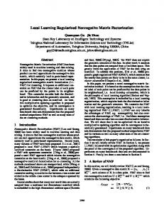
randomized model, the preliminary model obtained after several iterations of the EM procedure is more likely to be accurate, so that the WNMF approach is more likely to obtain a good local (or global) optimum. In short, such an approach not only has a high likelihood of obtaining accurate predictions, but reduces the computational cost as well. The performance of this hybrid approach appears promising based on our experiments. Figure 3 shows the results of combining the EM approach (with 1, 3, and 5 iterations) and the WNMF approach. 4.2 Results of the NMF based algorithms Table 1 summarizes the NMAE and ROC-4 area results obtained using different CF algorithms on MovieLens. The results show that the NMF-based EM approach and the SVD-based EM approach achieve the best result in NMAE, and the NMF-based EM approach achieves the best performance in ROC-4 area. The hybrid approach (with five iterations of the EM procedure plus the WNMF approach) also works very well. Table 2 shows the results obtained on Jester. Since the original rating range in Jester is from -10 to 10, we shift its range to [0, 20] for the NMF algorithm. One advantage of the NMF-based CF algorithms is that the coordinates obtained via NMF directly reflect the features of the user communities. By simply sorting each column in U , we get a characterization of each community in terms of the ranked list of preferences it has on all items. As an example, Figure 4 displays the five top ranked movies for five of the 20 user communities extracted from MovieLens. Generally, the

3 Each

iteration in the EM approach takes 303.3s and each updating round in WNMF takes 1.27s. The algorithms are implemented in Matlab R14, and the experiment was performed on a 2.8GHz Intel XEON machine with 4GB RAM.

551

Table 2: Performance of CF algorithms on Jester. NMAE ROC-4

Pearson 0.1634 0.7539

SVD EM 0.1605 0.7588

NMF EM 0.1599 0.7612

Hybrid NMF 0.1599 0.7608

Figure 4: The top five ranked movies in five of the 20 user communities extracted from MovieLens with NMF. The genres of movies as given by MovieLens are in parentheses. Some movies may have more than one genre. top movies in a given user community are in the same genre. For example, all the movies in group 8 are action movies, and all the movies in group 19 are musicals. We also see movies from the same series in some user groups—“Austin Powers” in group 5 and “Ace Ventura” in group 9. More surprisingly, some interesting features can be observed among movies in the same group, e.g., “Pretty Woman”, “Notting Hill”, “Steel Magnolias”, and “Erin Brockovich” in group 17 all feature Julia Roberts. The patterns and features extracted by NMF can be helpful in understanding shared interests of users and similarities among different items.

[8]

[9] [10]

[11] [12]

Acknowledgements This work is supported in part by the National Science Foundation under award number IDM 0308229. We thank the anonymous reviewers for their comments, which helped us improve the quality of the paper.

[13]

[14]

References [15] [1] C. C. Aggarwal, J. L. Wolf, K.-L. Wu, and P. S. Yu. Horting hatches an egg: A new graph-theoretic approach to collaborative filtering. In Proc. of the 5th ACM SIGKDD, 1999. [2] Y. Azar, A. Fiat, A. Karlin, F. McSherry, and J. Saia. Spectral analysis of data. In Proc. of the 33rd ACM STOC, 2001. [3] J. Canny. Collaborative filtering with privacy via factor analysis. In Proc. of the 25th ACM SIGIR, 2002. [4] A. P. Dempster, N. M. Laird, and D. B. Rubin. Maximum likelihood from incomplete data via the EM algorithm. J. of the Royal Statistical Society, 39:1–38, 1977. [5] K. Goldberg, T. Roeder, D. Gupta, and C. Perkins. Eigentaste: A constant time collaborative filtering algorithm. Information Retrieval, 4(2):133–151, 2001. [6] J. L. Herlocker, J. A. Konstan, A. Borchers, and J. Riedl. An algorithmic framework for performing collaborative filtering. In Proc. of the 22nd ACM SIGIR, 1999. [7] T. Hofmann. Latent semantic models for collabora-

552

[16]

[17]

[18]

[19] [20]

tive filtering. ACM Tran. on Information Systems, 22(1):89–115, 2004. D. D. Lee and H. S. Seung. Learning the parts of objects by non-negative matrix factorization. Nature, 401:788–791, 1999. D. D. Lee and H. S. Seung. Algorithms for nonnegative matrix factorization. NIPS, 13:556–562, 2001. Y. Mao and L. K. Saul. Modeling distances in largescale networks by matrix factorization. In Proc. of the 4th ACM SIGCOMM Conf. on Internet Measurement, 2004. B. Marlin. Modeling user rating profiles for collaborative filtering. In Proc. of the 17th NIPS, 2003. B. Marlin. Collaborative filtering: A machine learning perspective. Master’s thesis, University of Toronto, 2004. P. Paatero. Least squares forumulation of robust nonnegative factor analysis. Chemometrics and Intelligent Laboratory Systems, 37:23–35, 1997. P. Paatero and U. Tapper. Positive matrix factorization: A non-negative factor model with optimal utilization of error estimates of data values. Environmetrics, 5:127–144, 1994. D. M. Pennock, E. Horvitz, S. Lawrence, and C. L. Giles. Collaborative filtering by personality diagnosis: A hybrid memory and model-based approach. In Proc. of the 16th UAI, 2000. P. Resnick, N. Iacovou, M. Suchak, P. Bergstorm, and J. Riedl. GroupLens: An open architecture for collaborative filtering of netnews. In Proc. of ACM Conf. on Computer Supported Cooperative Work, 1994. B. M. Sarwar, G. Karypis, J. A. Konstan, and J. Reidl. Item-based collaborative filtering recommendation algorithms. In Proc. of the 10th WWW, 2001. B. M. Sarwar, G. Karypis, J. A. Konstan, and J. Riedl. Application of dimensionality reduction in recommender systems–a case study. In ACM WebKDD Workshop, 2000. N. Srebro and T. Jaakkola. Weighted low rank approximation. In Proc. of the 20th ICML, 2003. S. Zhang, W. Wang, J. Ford, F. Makedon, and J. Pearlman. Using singular value decomposition approximation for collaborative filtering. In Proc. of the 7th IEEE Conf. on E-Commerce, 2005.